Output Layer Structure Optimization for Weighted Regularized Extreme Learning Machine Based on Binary Method

Abstract

In this paper, we focus on the redesign of the output layer for the weighted regularized extreme learning machine (WRELM). For multi-classification problems, the conventional method of the output layer setting, named “one-hot method”, is as follows: Let the class of samples be r; then, the output layer node number is r and the ideal output of s-th class is denoted by the s-th unit vector in ${\mathbb{R}}^r$ ($1\le s\le r$). Here, in this article, we propose a “$binary$ $method$” to optimize the output layer structure: Let $2^{p-1}<r\le 2^p$, where $p\ge 2$, and p output nodes are utilized and, simultaneously, the ideal outputs are encoded in binary numbers. In this paper, the binary method is employed in WRELM. The weights are updated through iterative calculation, which is the most important process in general neural networks. While in the extreme learning machine, the weight matrix is calculated in least square method. That is, the coefficient matrix of the linear equations we solved is symmetric. For WRELM, we continue this idea. And the main part of the weight-solving process is a symmetry matrix. Compared with the one-hot method, the binary method requires fewer output layer nodes, especially when the number of sample categories is high. Thus, some memory space can be saved when storing data. In addition, the number of weights connecting the hidden and the output layer will also be greatly reduced, which will directly reduce the calculation time in the process of training the network. Numerical experiments are conducted to prove that compared with the one-hot method, the binary method can reduce the output nodes and hidden-output weights without damaging the learning precision.

1. Introduction

In the past few decades, the theory and application of artificial neural networks has developed rapidly because of their excellent approximation ability [1,2]. When training the network with the back propagation algorithm, it is very likely to fall into a local extremum and iteration is a time-consuming process. To avoid these shortcomings, Huang proposed the extreme learning machine (ELM) [3,4,5], and the weight matrix was calculated in least square method as an alternative to iterative computation. ELM was widely applied in many fields and achieved excellent results [6,7,8,9]. Based on the original ELM, some researchers added a weight factor and a regularization parameter to build the weighted regularized extreme learning machine (WRELM) [10,11]. The novel network can decrease the error caused by class-imbalanced samples in classification problems.

For the multi-classification problem, the common designs of output layer are one-versus-all (OVA) [12], one-versus-one (OVO) [13] and error-correcting output coding (ECOC) [14]. OVA transforms an r-classification problem into r parity problems, and the i-th classifier employs the i-th class samples as the positive samples and all the others as the negative samples. For OVO, two classes are in turn chosen to make a parity problem. Therefore, $r(r-1)/2$ classifiers are required for an r-classification problem. ECOC firstly designs a coding matrix M, and then decomposes the multi-classification problem into several parity problems; finally, it compares the hamming distance with the codes of each class to obtain the predicted value.

According to the OVA classification scheme, the conventional output layer design is one-hot method [15,16,17,18]: When solving r-classification problems $(r\ge 3)$, let the class of samples be r; then, the output layer node number is r and the ideal output of s-th class is denoted by s-th unit vector in ${\mathbb{R}}^r$ ($1\le s\le r$). For instance, when solving a 4-classification problem, the output node number is 4, and the samples of these four classes are labeled by $(1,0,0,0)$, $(0,1,0,0)$, $(0,0,1,0)$ and $(0,0,0,1)$, respectively. Obviously, the one-hot method requires too many output nodes, which leads to an excessive number of weights connecting the hidden and the output layers. And it seems too clumsy in terms of information storage. In the process of training the network, too many weights will inevitably consume too much computational time. The root of all these problems is the question of how to reduce the number of output nodes. We can derive some inspiration from the following two examples:

As we all know, for a parity problem [19], no one follows the one-hot method: no one prefers labeling the first class by $(1,0)$ and the second class by $(0,1)$. Instead of the one-hot method in this case, only one output node is employed, the first class is labeled by 1 and the second class is labeled by 0. Therefore, it seems that the one-hot method has some apparent shortages to be improved. Then, consider a general r-classification problem. Besides the one-hot method, we can also set the ideal output by the following process: Delete r-th output node; For the first $r-1$ classes of samples, we treat the problem as an $(r-1)$-classification problem and set the ideal outputs in one-hot method; Finally, for the last r-th class, set the ideal output to be (0, ⋯, 0)$\in {\mathbb{R}}^{r-1}$. This output layer design method can also solve the r-classification problem. Therefore, the one-hot method must not be the best.

The optimization of network structure can be mainly carried out from the following several aspects: input, hidden, output layers and weights. As an effective input layer optimization method, feature selection [20,21] is to select a subset of features that can represent the original data. Therefore, the dataset can be converted from high-dimensional to low dimensional space. For the hidden layer, regularization and its improved algorithm [22,23] are widely used to optimize the hidden layer of the network. Binarized neural network (BNN) [24,25] is a network that only uses $-1$ and $+1$ to represent the weights and activations. Based on the BNN, lots of researchers optimize the original network, mainly from the following aspects: minimizing the quantization [26,27], improving network loss function [28,29], and reducing the gradient error [30,31]. And in terms of application, BNN has also achieved good results [32,33,34]. Obviously, BNN can minimize the storage and the calculation of the model through binarizing the weights and activations into values $-1$ and $+1$.

Inspired by the above examples and binarized neural networks, the binary method is proposed instead of the one-hot method in this paper. The specific description of the binary method is as follows: Suppose $2^{p-1}<r\le 2^p$ with $p\ge 2$, and p output nodes are utilized and, simultaneously, the ideal outputs are encoded into binary numbers. Take the 4-classification problem as an example; two output nodes are needed, and these four classes are labeled by $(0,0)$, $(0,1)$, $(1,0)$ and $(1,1)$, respectively. It can be seen that when the class number is higher, the output node number that the binary method can reduce is greater. In the binary method, the output node number has been significantly reduced, which leads to a reduction in the number of hidden-output weights. In the storage process, lots of storage space will be saved. Moreover, in numerical experiments, the computational speed will also be improved because of the reduction of the weight number. The experiment part proves that compared with the conventional one-hot method, the binary method can reduce the output nodes and hidden-output weights without damaging the learning precision.

The remaining chapters are organized as follows: The description of the WRELM is given in Section 2. In the next section, the output layer designs under the one-hot and binary methods are introduced in detail. In Section 4, numerical experiments on six datasets are carried out after we show the experiment settings. Finally, the conclusion is presented in Section 5.

Throughout this paper, common notations for neural networks will be used. Some other symbols and their corresponding meanings are listed in

Table 1. Main symbols and their corresponding meanings.

Sign	Meaning	Sign	Meaning
${\mathbb{R}}^n$	n-dimensional vector space	$\mathsf{\Phi }$	data set
$\mathit{H}$	output matrix of hidden layer	${\mathit{H}}^T$	transpose of matrix $\mathit{H}$
${\mathit{H}}^{†}$	generalized inverse of matrix $\mathit{H}$	${\mathit{H}}^{-1}$	inverse of matrix $\mathit{H}$
$\mathit{I}$	identity matrix	C	regularization parameter
$\left|\right|·\left|\right|$	2-norm	g	sigmoid function

.

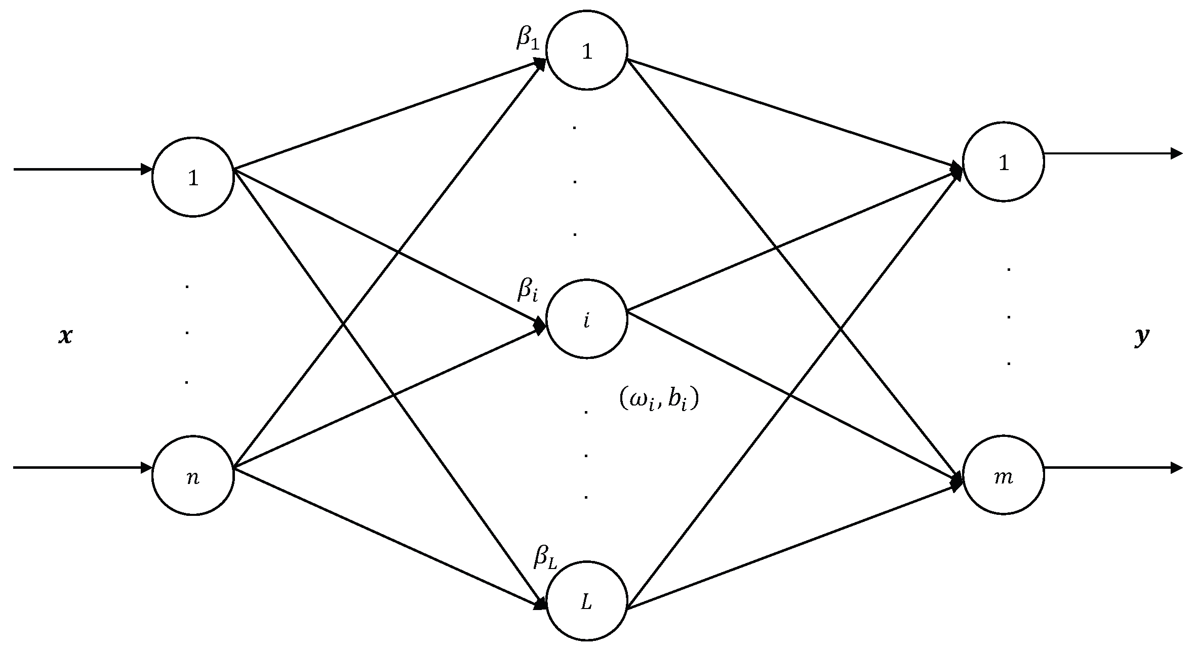
2. Brief Review of WRELM

Huang has proposed the ELM in [35,36,37], which is a type of single-layer feedforward neural network. In ELM, the basic idea is that the weights between input and hidden layers are randomly generated instead of iterative computational methods, and the weights between hidden and output layers are computed in the least square method.

Exhaustively, suppose that the input, hidden and output node numbers are n, L and m, respectively, which is demonstrated in Figure 1. The input $\mathit{x}\in {\mathbb{R}}^n$ is transformed into the hidden layer through random feature mapping; And the output value of the network is expressed by a linear combination of the mapped features. The specific formula is:

$$\mathit{y}=\sum _{i=1}^L{\beta }_i{g}_i\left(\mathit{x}\right)=\sum _{i=1}^L{\beta }_{i}g({\mathit{w}}_i·\mathit{x}+b_i),$$

(1)

where $\mathit{y}\in {\mathbb{R}}^m$ represents the actual output, ${\beta }_i={({\beta }_{i1},{\beta }_{i2},\dots ,{\beta }_{im})}^T\in {\mathbb{R}}^m$ is the weight vector connecting the i-th hidden node and the output nodes, ${\mathit{w}}_i={({\omega }_{i1},{\omega }_{i2},\dots ,{\omega }_{in})}^T$ is the weight vector connecting the input nodes and the i-th hidden node, $b_i$ is the bias of i-th hidden node and $g(·)$ is an activation function.

Given a sample set ${\left\{({\mathit{x}}_j,{\mathit{o}}_j)\right\}}_{j=1}^N$, where ${\mathit{x}}_j={(x_{j1},x_{j2},\dots ,x_{jn})}^T\in {\mathbb{R}}^n$ and ${\mathit{o}}_j={(o_{j1},o_{j2},\dots ,o_{jm})}^T$ $\in {\mathbb{R}}^m$, the corresponding j-th output node is:

$${\mathit{y}}_j=\sum _{i=1}^L{\beta }_{i}g({\mathit{w}}_i·{\mathit{x}}_j+b_i),\mathrm{for}j=1,\dots ,N.$$

(2)

Its purpose is to build a neural network that meets the conditions

$$\sum _{j=1}^N\left|\right|{\mathit{y}}_j-{\mathit{o}}_j\left|\right|=0,$$

(3)

which means finding ${\mathit{w}}_i$, ${\beta }_i$ and $b_i$ to satisfy

$$\sum _{i=1}^L{\beta }_{i}g({\mathit{w}}_i·{\mathit{x}}_j+b_i)={\mathit{o}}_j,\mathrm{for}j=1,\dots ,N.$$

(4)

These N equations mentioned above can be simplified to:

$$\mathit{H}\beta =\mathit{O},$$

(5)

where

$$\begin{array}{cc}\hfill & \mathit{H}({\mathit{w}}_1,{\mathit{w}}_2,\dots ,{\mathit{w}}_L,b_1,b_2,\dots ,b_L,{\mathit{x}}_1,{\mathit{x}}_2,\dots ,{\mathit{x}}_N)\hfill \\ \hfill & ={\left[\begin{array}{ccc}g({\mathit{w}}_1·{\mathit{x}}_1+b_1)& g({\mathit{w}}_2·{\mathit{x}}_1+b_2)\cdots & g({\mathit{w}}_L·{\mathit{x}}_1+b_L)\\ g({\mathit{w}}_1·{\mathit{x}}_2+b_1)& g({\mathit{w}}_2·{\mathit{x}}_2+b_2)\cdots & g({\mathit{w}}_L·{\mathit{x}}_2+b_L)\\ ⋮& \cdots & ⋮\\ g({\mathit{w}}_1·{\mathit{x}}_N+b_1)& g({\mathit{w}}_2·{\mathit{x}}_N+b_2)\cdots & g({\mathit{w}}_L·{\mathit{x}}_N+b_L)\end{array}\right]}_{N\times L},\hfill \end{array}$$

(6)

$$\beta ={\left[\begin{array}{c}{\beta }_1^T\\ ⋮\\ {\beta }_L^T\end{array}\right]}_{L\times m}\mathrm{and}\mathit{O}={\left[\begin{array}{c}{\mathit{o}}_1^T\\ ⋮\\ {\mathit{o}}_N^T\end{array}\right]}_{N\times m}.$$

(7)

In this paper, $\mathit{H}$ denotes the output matrix of the hidden layer. In the model of ELM, ${\mathit{w}}_i$ and ${\beta }_i$ ($i=1,\dots ,L$) are randomly generated instead of iterative computational methods. Therefore, the least square method is applied:

$$\beta =\left\{\begin{array}{c}{\left({\mathit{H}}^T\mathit{H}{\mathit{H}}^T\right)}^{-1}\mathit{O},\mathrm{if}L\le N,\hfill \\ {\left({\mathit{H}}^T\mathit{H}\right)}^{-1}\mathit{O},\mathrm{if}L>N.\hfill \end{array}\right.$$

(8)

In [36], Huang has proved the required hidden node number L must be less than or equal to the training sample number N. Therefore, for Equation (8), we take the case of $L\le N$. Obviously, ${\mathit{H}}^T\mathit{H}{\mathit{H}}^T$ is a symmetric matrix from a mathematical point of view. To simplify the formula, we write it as follows:

$$\beta ={\mathit{H}}^{†}\mathit{O},$$

(9)

where $\mathit{O}={[{\mathit{o}}_1,\dots ,{\mathit{o}}_N]}^T$, and ${\mathit{H}}^{†}$ stands for the Moore-Penrose generalized inverse of hidden layer output matrix $\mathit{H}$ [38,39].

Subsequently, in order to avoid the structure risk, some researchers proposed regularized extreme learning machine (RELM) [18,40,41] with a regularization parameter. The RELM can be expressed as

$$\min :\frac{1}{2}{\left|\right|\beta \left|\right|}^2+\frac{C}{2}{\left|\right|\epsilon \left|\right|}^2,$$

(10)

where C denotes the regularization parameter, ${\epsilon }_j={\sum }_{i=1}^{L}g({\mathit{w}}_j·{\mathit{x}}_j+b_j)-{\mathit{o}}_j$ is the sum of the training error; ${\left|\right|\epsilon \left|\right|}^2$ and ${\left|\right|\beta \left|\right|}^2$ are experience risk and structure risk, respectively. The output weight matrix is calculated by:

$$\beta ={({\mathit{H}}^T\mathit{H}+\frac{\mathit{I}}{C})}^{-1}{\mathit{H}}^T\mathit{O},$$

(11)

where $\mathit{I}$ denotes the identity matrix.

However, lots of imbalance classification problems actually exist. In other words, when solving a classification problem, it is not clear whether the data is class-balanced. If we treat the problem as class-balanced data, it may cause a large error. Therefore, we must use some measures to balance those classes with fewer samples. Based on the original RELM, we add a weight factor to build the WRELM [10,11]. As the process of RELM, the output weight matrix of WRELM is as follows:

$$\beta ={({\mathit{H}}^T{W}^2\mathit{H}+\frac{\mathit{I}}{C})}^{-1}{\mathit{H}}^T{W}^2\mathit{O},$$

(12)

where W is an $N\times N$ diagonal matrix. In order to decrease the role of $\mathit{I}$ played in (12), the value of C must be a big constant. The main part of (12) is a matrix with symmetry. Each main diagonal element of the diagonal matrix corresponds to its sample, and different classes of samples are automatically assigned different weights. Usually, we take an automatic weighting scheme [42]:

$$W_{ii}=\frac{1}{\mathrm{Count}\left({\mathit{o}}_i\right)},$$

(13)

where $W_{ii}$ is the i-th main diagonal element of W, $\mathrm{Count}\left({\mathit{o}}_i\right)$ denotes the sample number of class ${\mathit{o}}_i$.

With the above theory, the basic algorithm of WRELM is to calculate the output weight in the least square. The specific steps are as follows:

Step 1: Select the training set $\mathsf{\Phi }=\left\{({\mathit{x}}_j,{\mathit{o}}_j)\right|{\mathit{x}}_j\in {\mathbb{R}}^n,{\mathit{o}}_j\in {\mathbb{R}}^m,j=1,\dots ,N\}$. Choose the hidden node number L, regularization parameter C and the activation function $g(·)$;

Step 2: Randomly generate input weight ${\mathit{w}}_i$ and bias $b_i$, $i=1,\dots ,L$;

Step 3: Compute the output matrix $\mathit{H}$ of hidden layer;

Step 4: Compute the output weight matrix $\beta$ by (12).

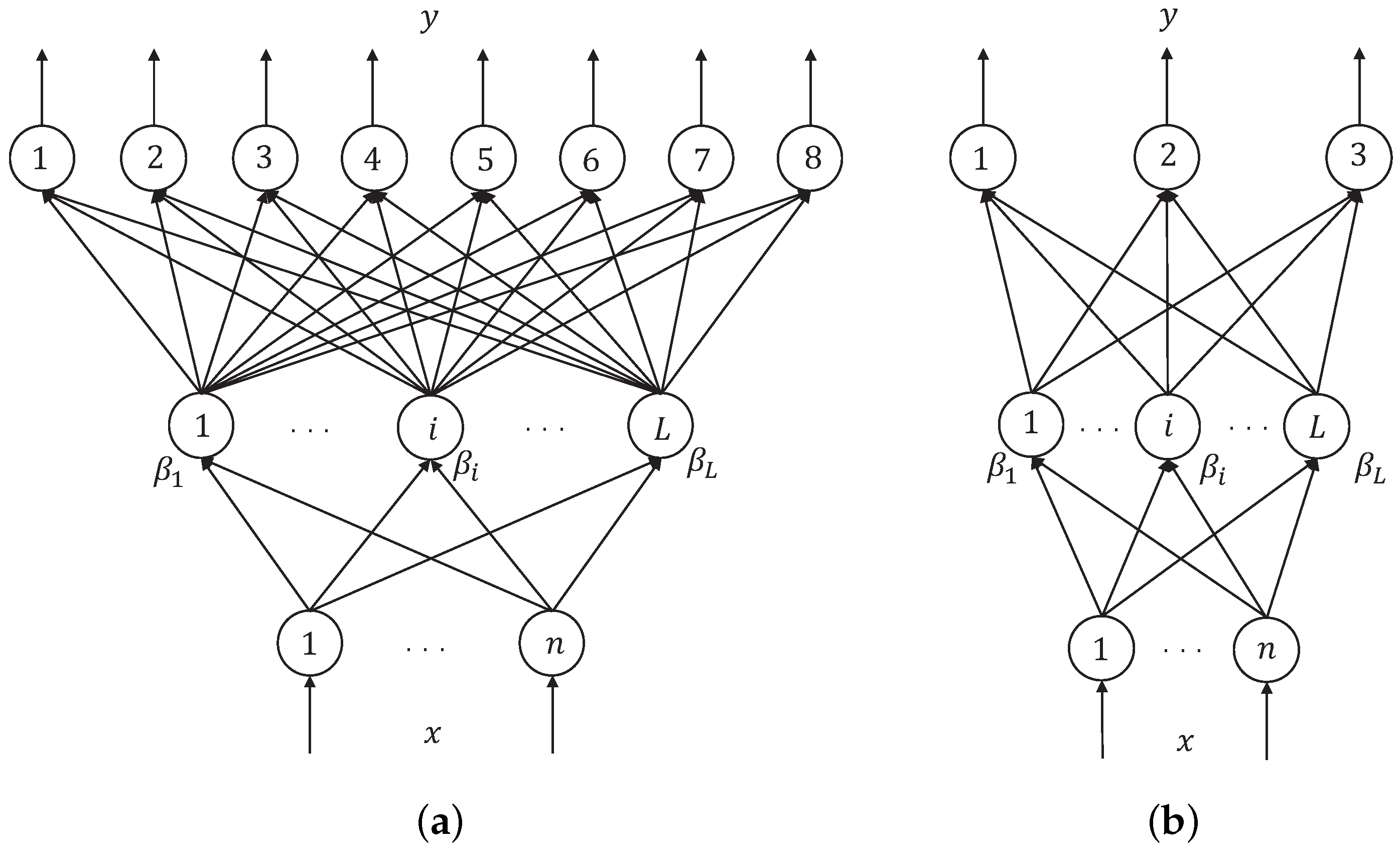
3. Output Layer Settings

In this section, two output layer settings are introduced: the conventional one-hot method and the novel proposed binary method.

3.1. One-Hot Method

When the conventional one-hot method is employed for an r-classification problem, if an input ${\mathit{x}}_j$ is a sample of s-th class, the ideal output ${\mathit{o}}_j$ will be

$$\begin{array}{cc}\hfill {\mathit{o}}_j& ={(o_{j1},o_{j2},\dots ,o_{j(s-1)},o_{js},o_{j(s+1)},\dots ,o_{jr})}^T\hfill \\ \hfill & ={(0,0,\dots ,0,1,0,\dots ,0)}^T.\hfill \end{array}$$

(14)

In other words, an input ${\mathit{x}}_j\in {\mathbb{R}}^n$ can be assigned to the s-th class, if the final actual output (2) of the network satisfies:

$$\begin{array}{cc}\hfill {\mathit{y}}_j& ={(y_{j1},y_{j2},\dots ,y_{j(s-1)},y_{js},y_{j(s+1)},\dots ,y_{jr})}^T\hfill \\ \hfill & \approx {(0,0,\dots ,0,1,0,\dots ,0)}^T.\hfill \end{array}$$

(15)

The one-hot method is considered to effectively solve a classification problem if the input sample belonging to the s-th class satisfies Equation (15) for each $s=1,\dots ,r$. If the input sample satisfies Equation (15) for each $s=1,\dots ,r$, then it belongs to the s-th class.

3.2. Binary Method

Now, we proceed to introduce the new binary method: Let $2^{p-1}<r\le 2^p$ with $p\ge 2$. Thus, the number of output nodes will be reduced to p. And for each class of samples, the binary manner is applied to encode the ideal outputs: The ideal output of the s-th class is

$${\mathit{o}}_j\left(s\right)={(o_{j1},o_{j2},\dots ,o_{jp})}^T,$$

(16)

where

$$o_{j1}{o}_{j2}\cdots o_{jp}={(s-1)}_2.$$

(17)

In Equation (17), ${(s-1)}_2$ represents the binary number of $(s-1)$, where $o_{jk}=1$ or 0, $1\le k\le p$. Analogously, we claim that the binary method successfully solves a classification problem if the input sample belonging to the s-th class satisfies for $s=1,\dots ,r$:

$${(y_{j1},y_{j2},\dots ,y_{jq})}^T\approx {\mathit{o}}_j\left(s\right).$$

(18)

The above binary method indeed needs a smaller amount of output nodes than the one-hot method. In order to visualize the advantages of the binary method, we take the eight-classification problem as an example. There should be eight output nodes in the one-hot method (cf. Figure 2a), while only three output nodes are needed in the binary method (cf. Figure 2b). Moreover, the number of hidden-output weights is also reduced, which will result in a significant reduction in computational time.

Remark 1.

In the one-hot method, an input ${\mathit{x}}_j\in {\mathbb{R}}^n$ can be assigned to the s-th class, if the final actual output of the network satisfies [43]:

$$y_{js}=max\left\{{\mathit{y}}_j\right\}.$$

(19)

However, the one-hot method has an obvious disadvantage. This method may fail to classify the sample if the actual output has another node equal or approximate to the maximum value:

$$y_{j{s}^{\prime }}=y_{js}\mathrm{or}{y}_{j{s}^{\prime }}\approx y_{js},s\ne s^{\prime }.$$

(20)

For example, when solving a two-class classification problem, we will classify a sample into the second class if its actual output is $(0.92,0.93)$. However, the possibility that this sample belongs to the first class is also especially high.

Another criterion to classify a sample is as follows: Evaluate the value of each output node, and then transform each output node to value 0 or 1. (In next section, we will give a criterion about the transformation.) Under this criterion, we cannot say the sample belongs to the first or the second class if the actual output is $(0.92,0.93)$.

One way of circumventing these difficulties is to replace the one-hot method with the binary method. When solving a four-classification problem, we can easily classify the sample into the fourth class if the actual output is $(0.92,0.93)$. When the actual output has another node equal or nearly equal to the maximum value, the one-hot method fails to classify this sample accurately, but the binary method succeeds.

4. Numerical Experiments

To verify the validity of the binary method, we compare it with the one-hot method on six real multi-classification problems: Wine [44], Car [45], image segmentation (IS) [46], four-class sensorless drive diagnosis (FSDD) [47], crowdsourced mapping (CM) [48], and letter recognition (LR) [49]. All the experiments below are conducted in Matlab 2014a, and the computer is a Macbook pro 2015.

4.1. Experiment Settings

In our experiments, five-fold cross validation technology will be used [50,51,52,53] in both the one-hot and binary methods. For details, the dataset is equally divided into five parts, and the learning process is conducted twenty times. For each time the training process is run, each part takes turns as the test set, while the rest are used as the training sets. The above processes are repeated 20 times. After adding them all together, one hundred classification results are achieved for each method-data pair.

We evaluate the class of a sample according to the actual output by the standards: If the actual output is less than $0.50$, then we regard it as approximately equal to 0; And if the actual output is more than $0.50$, then we regard it as approximately equal to 1. Here, the sigmoidal function is employed as an activation function:

$$g\left(x\right)=\frac{1}{1+e^{-x}}.$$

(21)

For WRELM, the input-hidden weights are stochastically generated and fixed in the subsequent learning procedure; then, the hidden-output weights are calculated in least square method rather than iterative methods. Therefore, there are two parameters in WRELM: hidden node number L and regularization parameter C. In [36], Huang provided the theorem that the required hidden node number L must be less than or equal to the training sample number N. Moreover in [35], Huang gave the explanation that $L\ll N$ under normal circumstances.

The experiment process is given in the following Algorithm 1:

Algorithm 1 Experiment process

Step 1: Input the dataset $\mathsf{\Phi }=\left\{({\mathit{x}}_j,{\mathit{o}}_j)\right|{\mathit{x}}_j\in {\mathbb{R}}^n,{\mathit{o}}_j\in {\mathbb{R}}^m,j=1,\dots ,N\}$ and regularization parameter C. For each class, input the ideal outputs in both the one-hot and binary methods. Step 2: $\mathit{Five}$-fold cross validation technology: $\mathsf{\Phi }=\left\{({\mathit{x}}_j,{\mathit{o}}_j)\right|{\mathit{x}}_j\in {\mathbb{R}}^n,{\mathit{o}}_j\in {\mathbb{R}}^m,j=1,\dots ,N\}$ is equally divided into five parts: ${\mathsf{\Phi }}_1$, …, ${\mathsf{\Phi }}_5$. Step 3: For $i=1$ to $i=5$, do Step 3 to Step 7. Let ${\mathsf{\Phi }}_i$ be the test samples, while $\mathsf{\Phi }\backslash {\mathsf{\Phi }}_i$ is the training samples. Step 4: Compute the hidden layer output matrix $\mathit{H}$ by Equation (6); next, calculate the output weight $\beta$ (cf. Equation (12)) according to the training samples. Step 5: Compute the actual outputs (cf. Equation (2)) of the test samples. Step 6: For each sample, calculate the approximate value of the actual output according to the approximation criteria given before, and calculate the classification accuracies. Step 7: Repeat the above procedure twenty times. Step 8: Let $L=L+L_0$, where $L_0$ is the step and the initial value of L is a small positive integer. Repeat Step 3 to Step 7 until L attains half of the training sample number. Step 9: For each value of L, choose the optimal accuracies and calculate the average accuracies. Step 10: Draw figures and tables according to the one hundred experimental results obtained in Step 9, and then compare the performances of one-hot and binary methods.

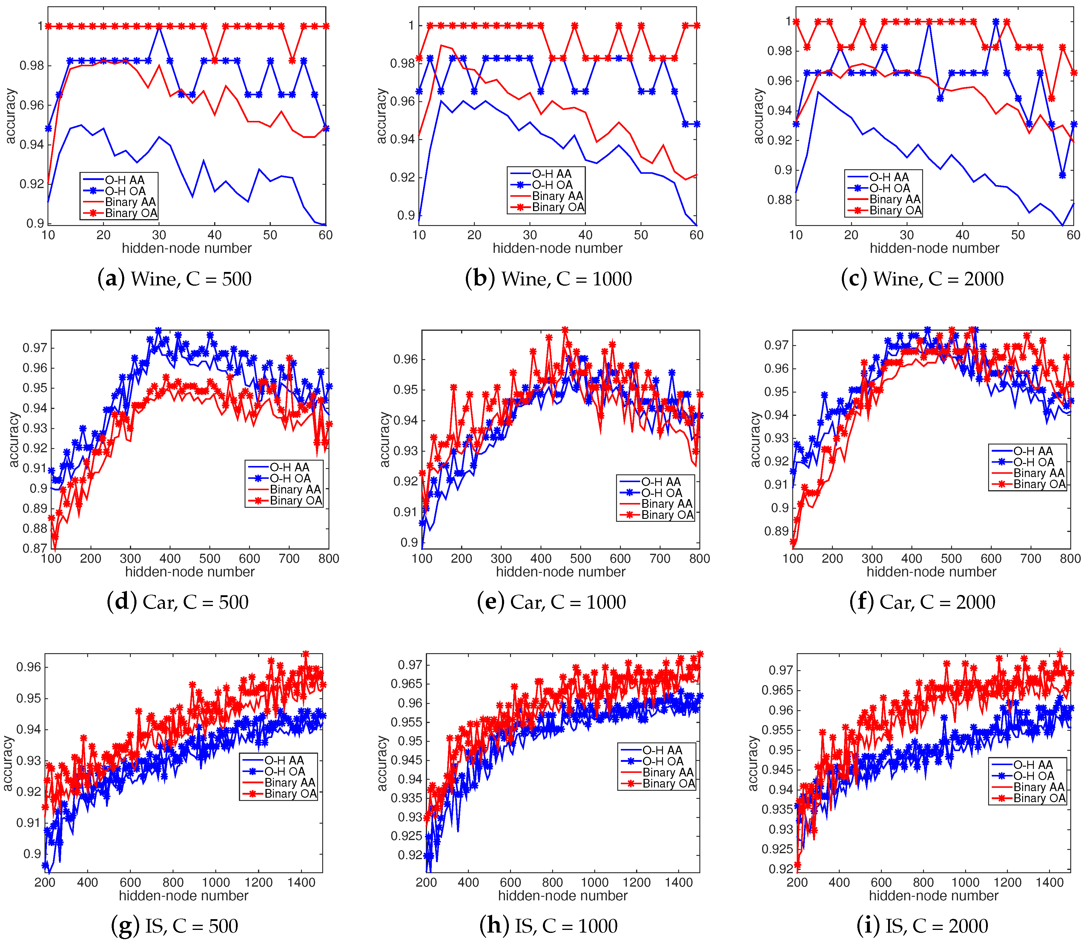
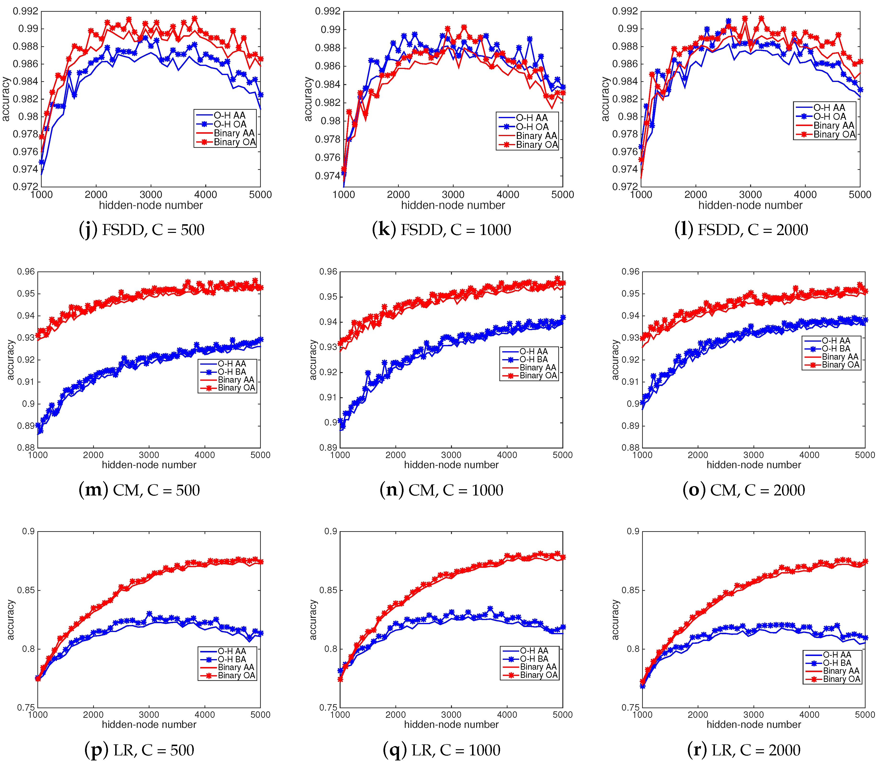
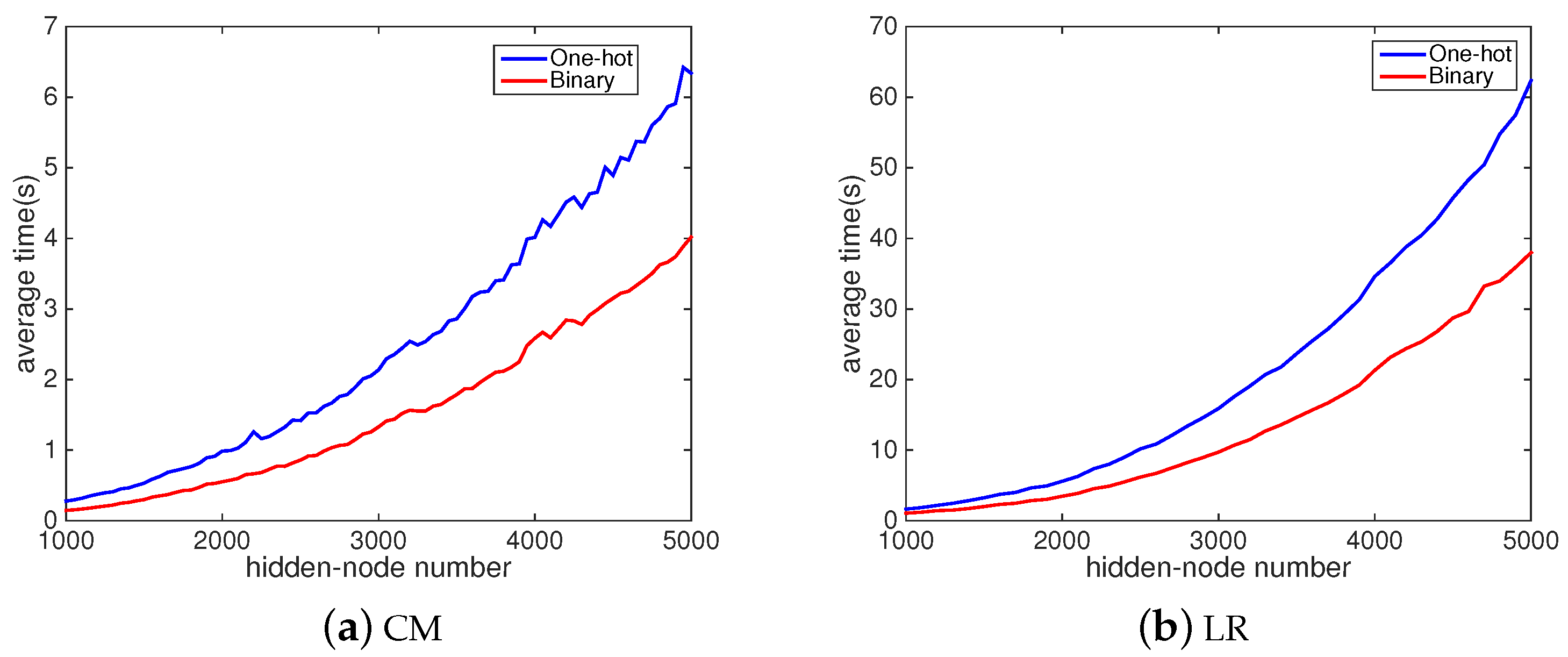
4.2. Classification Accuracies and Computational Time

In

Table 2. Test accuracies for six different datasets.

Dataset	Class	Attribute	Case	O-H		Binary
				AA	OA	AA	OA
			SVM	94.16%	97.42%	95.53%	98.28%
			APNN	94.30%	98.28%	96.06%	100.00%
			ELM	94.71%	100.00%	96.19%	100.00%
Wine	4	13	WELM, C = 0	95.04%	98.28%	97.16%	100.00%
			WRELM, C = 500	95.00%	100.00%	98.28%	100.00%
			WRELM, C = 1000	96.03%	98.28%	97.16%	100.00%
			WRELM, C = 2000	95.26%	100.00%	97.16%	100.00%
			SVM	93.59%	94.07%	93.46%	94.05%
			APNN	94.27%	95.62%	94.78%	96.11%
			ELM	96.54%	97.90%	94.86%	96.73%
Car	4	6	WELM, C = 0	97.03%	98.11%	97.12%	98.04%
			WRELM, C = 500	97.27%	97.90%	94.94%	96.50%
			WRELM, C = 1000	95.56%	96.03%	96.34%	96.96%
			WRELM, C = 2000	97.12%	97.66%	96.94%	97.66%
			SVM	93.54%	93.91%	94.70%	95.26%
			APNN	94.02%	94.35%	95.39%	96.71%
			ELM	94.69%	95.43%	96.12%	97.04%
IS	7	18	WELM, C = 0	95.37%	95.91%	96.49%	97.17%
			WRELM, C = 500	94.38%	94.59%	95.70%	96.44%
			WRELM, C = 1000	96.11%	96.31%	96.93%	97.30%
			WRELM, C = 2000	95.90%	96.34%	96.89%	97.43%
			SVM	96.78%	97.51%	97.03%	97.84%
			APNN	97.28%	97.90%	97.50%	98.21%
			ELM	98.80%	99.03%	98.91%	99.09%
FSDD	4	48	WELM, C = 0	98.80%	99.01%	98.82%	99.06%
			WRELM, C = 500	98.73%	98.90%	99.01%	99.12%
			WRELM, C = 1000	98.82%	98.95%	98.80%	99.03%
			WRELM, C = 2000	98.83%	99.09%	99.02%	99.12%
			SVM	91.04%	91.60%	92.86%	93.37%
			APNN	91.90%	92.35%	93.67%	94.02%
			ELM	92.67%	93.18%	94.58%	95.15%
CM	6	28	WELM, C = 0	92.81%	93.76%	94.97%	95.28%
			WRELM, C = 500	92.66%	92.93%	95.35%	95.61%
			WRELM, C = 1000	93.96%	94.20%	95.48%	95.75%
			WRELM, C = 2000	93.71%	93.92%	95.05%	95.43%
			SVM	81.36%	82.13%	81.71%	82.64%
			APNN	82.72%	83.41%	82.94%	83.79%
			ELM	81.57%	82.60%	87.60%	87.96%
LR	26	16	WELM, C = 0	81.83%	82.35%	87.32%	87.81%
			WRELM, C = 500	82.30%	83.04%	87.44%	87.68%
			WRELM, C = 1000	82.75%	83.46%	87.78%	88.14%
			WRELM, C = 2000	81.79%	82.08%	87.24%	87.60%

, we choose the optimal accuracy (OA) and calculate the average accuracy (AA) according to the one hundred results in support vector machine (SVM), associative pulsing neural network (APNN), ELM and WRELM. Make a longitudinal contrast to the classification accuracies in Table 2. The sequence of these four classifiers is: WRELM > ELM > APNN > SVM.

After verifying the role of the weighted matrix, we turn to compare the classification accuracies of one-hot and binary methods. Obviously, the binary method outperforms the one-hot (O-H) method in four (Wine, IS, CM and LR) out of the six test datasets no matter which regularization parameter is chosen. More precisely, in terms of the OA, only when the binary reaches 100% accuracy may the one-hot method have the same excellent performances. For the Car problem, the one-hot method outperforms the binary method in eight out of the fourteen classification accuracies (AA and OA in seven network models). Moreover, for the FSDD problem, the binary method is absolutely better than the one-hot method in thirteen cases; only in the case $C=1000$, the AA of the one-hot method is just 0.02% higher than that of the binary method; And on the aspect of OA, the one-hot method is 0.08% lower than the binary method. From the overall experimental results, the performances of the binary method are slightly worse than the one-hot method in only one dataset (car), while the performances are far better than the one-hot method in the other five datasets of the experiments.

Figure 3 exhibits the OA and AA with different hidden-node numbers and regularization parameters. Overall, eighteen-pair experiment results are obtained: The binary method can achieve obviously higher accuracies than the one-hot method in thirteen (case: a, b, c, g, h, i, j, m, n, o, p, q, r) out of the eighteen cases, while the binary method performs worse only in case d; And for the rest of the four cases (case: e, f, k, l), the accuracies of these two methods are similar, one is never better than the other.

Experimental results reveal that, on the aspect of classification accuracy, the binary method performs significantly better than the one-hot method.

Moreover, the binary method indeed requires less output nodes than the one-hot method especially when the class number is high. Therefore, the WRELM in the binary approach has a faster computational speed than the one-hot method. Since this result is obvious, we only selected CM and LR datasets as examples. And the computational time comparison of these two methods is shown in Figure 4.

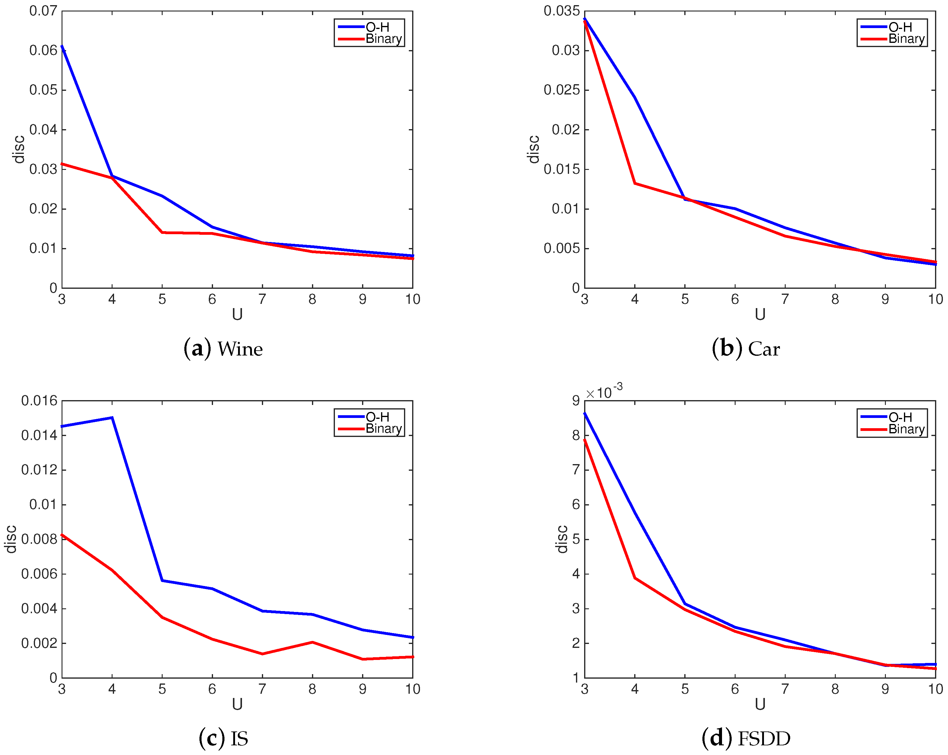
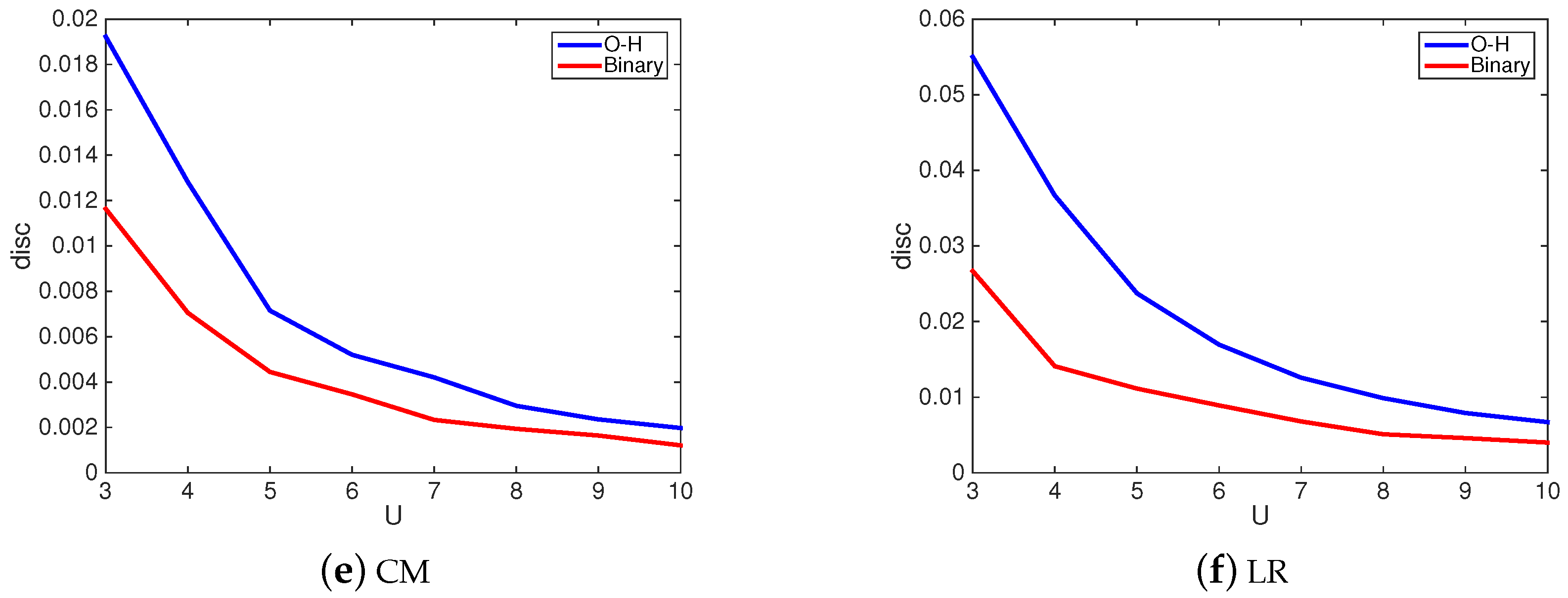
4.3. Comparison on Several Evaluation Criteria

For the purpose of evaluating the error in the learning process of these two methods, besides the classification accuracy, we also compare the following five criteria: prediction rate (PR), recalling rate (RR) [54], and F1-measure [55], the standard deviation ($\sigma$) [56] and the root mean square error (RMSE) [57]. Since the prediction and recall rate are defined for parity problems, while dealing with multi-classification problems, we extend the original definition: For an r-classification problem, $i\in \{1,2,\cdots ,r\}$, we regard the samples of i-th class as a positive set while the remaining one is classified as negative; Compute ${\mathrm{PR}}_i$ and ${\mathrm{RR}}_i$; Repeat r times and calculate the average PR and RR. S is the number of the training samples. The specific calculation formulas are as follows:

$$\begin{array}{cc}\hfill \sigma :=& \sqrt{\frac{1}{S-1}\sum _{i=1}^{S-1}\frac{1}{r}\sum _{j=1}^r{(y_{ij}-\overline{y_{ij}})}^2};\hfill \\ \hfill \mathrm{RMSE}:=& \sqrt{\frac{1}{S}\sum _{i=1}^S\frac{1}{r}\sum _{j=1}^r{(y_{ij}-o_{ij})}^2};\hfill \\ \hfill \mathrm{PR}:=& \frac{1}{r}\sum _{i=1}^r\frac{{\mathrm{TP}}_i}{{\mathrm{TP}}_i+{\mathrm{FP}}_i};\hfill \\ \hfill \mathrm{RR}:=& \frac{1}{r}\sum _{i=1}^r\frac{{\mathrm{TP}}_i}{{\mathrm{TP}}_i+{\mathrm{FN}}_i};\hfill \\ \hfill \mathrm{F}1:=& \frac{2\times \mathrm{PR}\times \mathrm{RR}}{\mathrm{PR}+\mathrm{RR}}.\hfill \end{array}$$

And

Table 3. Some criteria on six datasets.

Dataset	O-H					Binary
	PR	RR	F1	σ	RMSE	PR	RR	F1	σ	RMSE
Wine	95.67%	94.89%	95.28%	0.0238	0.0167	98.48%	97.03%	97.75%	0.0202	0.0116
Car	93.97%	93.15%	93.56%	0.0210	0.0152	92.45%	91.40%	91.92%	0.0255	0.0171
IS	94.39%	94.71%	94.55%	0.0169	0.0175	96.38%	96.23%	96.30%	0.0108	0.0130
FSDD	98.56%	99.04%	98.80%	0.0123	0.0047	99.09%	98.60%	98.84%	0.0094	0.0037
CM	92.94%	84.16%	88.33%	0.0153	0.0124	94.51%	88.79%	91.56%	0.0105	0.0097
LR	84.72%	70.04%	76.68%	0.0092	0.0021	89.94%	72.61%	80.35%	0.0071	0.0015

shows the prediction rate, recall rate, F1, $\sigma$, and RMSE of these two methods. In the datasets of Wine, IS, CM and LR, the binary method has better performances on all the $\mathit{five}$ criteria than the one-hot method. Only in the dataset of Car, the one-hot method has better performances on $\mathit{five}$ criteria than our binary method. And for the rest of the FSDD dataset, only in the criterion of recall accuracy does the one-hot method have a slightly better performance, while the binary method performs better on all the other four criteria.

4.4. Sensitivity Analysis

For a certain multi-classification problem, it is hard to give the optimal hidden node number accurately. We hope that the hidden node number has as little impact on the experimental results as possible. Therefore, we compare the sensitivity of these two methods and the procedure is as follows: Averagely select U points from the range of the hidden node number (see Figure 3); Next calculate the sum of the accuracy discrepancies between any two adjacent points for the WRELM with both the one-hot and binary methods. Repeat the above procedure $K=100$ times and average the cases $C=500,1000,2000$. Finally, we obtain the average accuracy discrepancy:

$$\mathrm{disc}\left(U\right)=\frac{1}{K(U-1)}\sum _{k=1}^K\sum _{u=1}^{U-1}|\mathrm{acc}\left(n_{u+1}^{\left(k\right)}\right)-\mathrm{acc}\left(n_u^{\left(k\right)}\right)|,$$

where $n_1^{\left(k\right)},\cdots ,n_U^{\left(k\right)}$ represent the U points averagely taken from the k-th iteration, and $\mathrm{acc}\left(x\right)$ represents the accuracy at the point x. From a mathematical point of view, the smaller value of $\mathrm{disc}\left(U\right)$ means that the hidden node number has less influence on the classification accuracies.

In our experiments, each value in set $\{3,4,\cdots ,10\}$ is assigned to U, respectively. As shown in Figure 5, in terms of experimental sensitivity, the binary method performs better than the one-hot method on all of these six datasets. Thus, compared with the one-hot method, the choice of hidden number has a smaller effect on classification accuracy in the binary method.

5. Conclusions

The binary method applied on the output layer to optimize the structure of the network is considered in this paper. When WRELM is employed to deal with a multi-classification problem, the common and conventional one-hot method is applied. However, too many output nodes and hidden-output weights are needed, which will waste too much computational time. As a remedy, we propose a binary method: let $2^{p-1}<r\le 2^p$, where $p\ge 2$, and p output nodes are utilized and simultaneously the ideal outputs are encoded in binary numbers. Compared with the one-hot method, the novel binary method requires fewer output nodes, which will result in a great decrease in the weight number. And in the process of training the network, the binary method has a higher computational efficiency than the one-hot method.

Experiments are conducted for solving six-real multi-classification problems. The experimental results reveal that the binary method can achieve higher classification accuracies and faster computational speed than the traditional one-hot method. Combined with the theory and experimental results, the binary method can not only optimize the output layer structure, but also improve the comprehensive classification performances of WRELM.

References

1. Faris, H.; Aljarah, I.; Mirjalili, S. Training feedforward neural networks using multi-verse optimizer for binary classification problems. Appl. Intell. 2016, 45, 322–332. [Google Scholar] [CrossRef]
2. Eldan, R.; Shamir, O. The power of depth for feedforward neural networks. In Proceedings of the Conference on Learning Theory, New York, NY, USA, 23–26 June 2016; pp. 907–940. [Google Scholar]
3. Huang, G.B.; Zhou, H.; Ding, X.; Zhang, R. Extreme learning machine for regression and multiclass classification. IEEE Trans. Syst. Man Cybern. Part B 2011, 42, 513–529. [Google Scholar] [CrossRef] [PubMed] [Green Version]
4. Sattar, A.M.; Ertuğrul, Ö.F.; Gharabaghi, B.; McBean, E.A.; Cao, J. Extreme learning machine model for water network management. Neural Comput. Appl. 2019, 31, 157–169. [Google Scholar] [CrossRef]
5. Dai, H.; Cao, J.; Wang, T.; Deng, M.; Yang, Z. Multilayer one-class extreme learning machine. Neural Netw. 2019, 115, 11–22. [Google Scholar] [CrossRef] [PubMed]
6. Yaseen, Z.M.; Sulaiman, S.O.; Deo, R.C.; Chau, K.W. An enhanced extreme learning machine model for river flow forecasting: State-of-the-art, practical applications in water resource engineering area and future research direction. J. Hydrol. 2019, 569, 387–408. [Google Scholar] [CrossRef]
7. Luo, X.; Jiang, C.; Wang, W.; Xu, Y.; Wang, J.H.; Zhao, W. User behavior prediction in social networks using weighted extreme learning machine with distribution optimization. Future Gener. Comput. Syst. 2019, 93, 1023–1035. [Google Scholar] [CrossRef]
8. Zhang, D.; Peng, X.; Pan, K.; Liu, Y. A novel wind speed forecasting based on hybrid decomposition and online sequential outlier robust extreme learning machine. Energy Convers. Manag. 2019, 180, 338–357. [Google Scholar] [CrossRef]
9. Cao, F.; Yang, Z.; Ren, J.; Chen, W.; Han, G.; Shen, Y. Local block multilayer sparse extreme learning machine for effective feature extraction and classification of hyperspectral images. IEEE Trans. Geosci. Remote Sens. 2019, 57, 5580–5594. [Google Scholar] [CrossRef] [Green Version]
10. Ding, S.; Ma, G.; Shi, Z. A rough RBF neural network based on weighted regularized extreme learning machine. Neural Process. Lett. 2014, 40, 245–260. [Google Scholar] [CrossRef]
11. Huang, N.; Yuan, C.; Cai, G.; Xing, E. Hybrid short term wind speed forecasting using variational mode decomposition and a weighted regularized extreme learning machine. Energies 2016, 9, 989. [Google Scholar] [CrossRef]
12. Belghit, A.; Lazri, M.; Ouallouche, F.; Labadi, K.; Ameur, S. Optimization of One versus All-SVM using AdaBoost algorithm for rainfall classification and estimation from multispectral MSG data. Adv. Space Res. 2023, 71, 946–963. [Google Scholar] [CrossRef]
13. Pawara, P.; Okafor, E.; Groefsema, M.; He, S.; Schomaker, L.R.; Wiering, M.A. One-vs-One classification for deep neural networks. Pattern Recognit. 2020, 108, 107528. [Google Scholar] [CrossRef]
14. Liu, K.H.; Gao, J.; Xu, Y.; Feng, K.J.; Ye, X.N.; Liong, S.T.; Chen, L.Y. A novel soft-coded error-correcting output codes algorithm. Pattern Recognit. 2023, 134, 109122. [Google Scholar] [CrossRef]
15. Nie, Q.; Jin, L.; Fei, S.; Ma, J. Neural network for multi-class classification by boosting composite stumps. Neurocomputing 2015, 149, 949–956. [Google Scholar] [CrossRef]
16. Lei, Y.; Dogan, Ü.; Zhou, D.X.; Kloft, M. Data-dependent generalization bounds for multi-class classification. IEEE Trans. Inf. Theory 2019, 65, 2995–3021. [Google Scholar] [CrossRef] [Green Version]
17. Tang, L.; Tian, Y.; Pardalos, P.M. A novel perspective on multiclass classification: Regular simplex support vector machine. Inf. Sci. 2019, 480, 324–338. [Google Scholar] [CrossRef]
18. Dong, Q.; Zhu, X.; Gong, S. Single-label multi-class image classification by deep logistic regression. In Proceedings of the AAAI Conference on Artificial Intelligence, Honolulu, HI, USA, 27 January–1 February 2019; Volume 33, pp. 3486–3493. [Google Scholar]
19. Ruivo, E.L.; de Oliveira, P.P. A perfect solution to the parity problem with elementary cellular automaton 150 under asynchronous update. Inf. Sci. 2019, 493, 138–151. [Google Scholar] [CrossRef]
20. Saberi-Movahed, F.; Rostami, M.; Berahmand, K.; Karami, S.; Tiwari, P.; Oussalah, M.; Band, S.S. Dual regularized unsupervised feature selection based on matrix factorization and minimum redundancy with application in gene selection. Knowl.-Based Syst. 2022, 256, 109884. [Google Scholar] [CrossRef]
21. Rostami, M.; Berahmand, K.; Nasiri, E.; Forouzandeh, S. Review of swarm intelligence-based feature selection methods. Eng. Appl. Artif. Intell. 2021, 100, 104210. [Google Scholar] [CrossRef]
22. Wang, L.; Zhou, H.; Chen, H.; Wang, Y.; Zhang, Y. Structure-Guided L1/2 Minimization for Stable Multichannel Seismic Attenuation Compensation. IEEE Trans. Geosci. Remote Sens. 2022, 60, 1–9. [Google Scholar] [CrossRef]
23. Heydari, E.; Abadi, M.S.E.; Khademiyan, S.M. Improved multiband structured subband adaptive filter algorithm with L0-norm regularization for sparse system identification. Digit. Signal Process. 2022, 122, 103348. [Google Scholar] [CrossRef]
24. Courbariaux, M.; Bengio, Y. BinaryConnect: Training Deep Neural Networks with Binary Weights during Propagations; MIT Press: Cambridge, MA, USA, 2015. [Google Scholar]
25. Courbariaux, M.; Hubara, I.; Soudry, D.; El-Yaniv, R.; Bengio, Y. Binarized Neural Networks: Training Deep Neural Networks with Weights and Activations Constrained to +1 or −1. arXiv 2016, arXiv:1602.02830. [Google Scholar]
26. Rastegari, M.; Ordonez, V.; Redmon, J.; Farhadi, A. XNOR-Net: ImageNet Classification Using Binary Convolutional Neural Networks; Springer: Cham, Switzerland, 2016. [Google Scholar]
27. Chitrakar, P.; Zhang, C.; Warner, G.; Liao, X. Social Media Image Retrieval Using Distilled Convolutional Neural Network for Suspicious e-Crime and Terrorist Account Detection. In Proceedings of the 2016 IEEE International Symposium on Multimedia (ISM), San Jose, CA, USA, 11–13 December 2016. [Google Scholar]
28. Lu, H.; Yao, Q.; Kwok, J.T. Loss-aware Binarization of Deep Networks. In Proceedings of the 5th International Conference on Learning Representations (ICLR 2017), Toulon, France, 24–26 April 2017. [Google Scholar]
29. Hartmann, M.; Farooq, H.; Imran, A. Distilled Deep Learning based Classification of Abnormal Heartbeat Using ECG Data through a Low Cost Edge Device. In Proceedings of the 2019 IEEE Symposium on Computers and Communications (ISCC), Barcelona, Spain, 29 June–3 July 2019. [Google Scholar]
30. Darabi, S.; Belbahri, M.; Courbariaux, M.; Nia, V.P. BNN+: Improved Binary Network Training. arXiv 2018, arXiv:1812.11800. [Google Scholar]
31. Liu, C.; Ding, W.; Xia, X.; Zhang, B.; Gu, J.; Liu, J.; Ji, R.; Doermann, D. Circulant Binary Convolutional Networks: Enhancing the Performance of 1-bit DCNNs with Circulant Back Propagation. In Proceedings of the IEEE/CVF Conference on Computer Vision and Pattern Recognition, Long Beach, CA, USA, 16–17 June 2019. [Google Scholar]
32. Kung, J.; Zhang, D.; Gooitzen, V.; Chai, S.; Mukhopadhyay, S. Efficient Object Detection Using Embedded Binarized Neural Networks. J. Signal Process. Syst. 2017, 90, 877–890. [Google Scholar] [CrossRef]
33. Leng, C.; Li, H.; Zhu, S.; Jin, R. Extremely Low Bit Neural Network: Squeeze the Last Bit Out with ADMM. In Proceedings of the Thirty-Second AAAI Conference on Artificial Intelligence, San Francisco, CA, USA, 4–9 February 2017. [Google Scholar]
34. Li, R.; Wang, Y.; Liang, F.; Qin, H.; Fan, R. Fully Quantized Network for Object Detection. In Proceedings of the 2019 IEEE/CVF Conference on Computer Vision and Pattern Recognition (IEEE CVPR), Long Beach, CA, USA, 15–20 June 2019. [Google Scholar]
35. Huang, G.B.; Zhu, Q.Y.; Siew, C.K. Extreme learning machine: A new learning scheme of feedforward neural networks. Neural Netw. 2004, 2, 985–990. [Google Scholar]
36. Huang, G.B.; Zhu, Q.Y.; Siew, C.K. Extreme learning machine: Theory and applications. Neurocomputing 2006, 70, 489–501. [Google Scholar] [CrossRef]
37. Huang, G.B.; Wang, D.H.; Lan, Y. Extreme learning machines: A survey. Int. J. Mach. Learn. Cybern. 2011, 2, 107–122. [Google Scholar] [CrossRef]
38. Fill, J.A.; Fishkind, D.E. The Moore–Penrose Generalized Inverse for Sums of Matrices. SIAM J. Matrix Anal. Appl. 2000, 21, 629–635. [Google Scholar] [CrossRef] [Green Version]
39. Rakha, M.A. On the Moore–Penrose generalized inverse matrix. Appl. Math. Comput. 2004, 158, 185–200. [Google Scholar] [CrossRef]
40. Cosmo, D.L.; Salles, E.O.T. Multiple Sequential Regularized Extreme Learning Machines for Single Image Super Resolution. IEEE Signal Process. Lett. 2019, 26, 440–444. [Google Scholar] [CrossRef]
41. Yu, Q.; Miche, Y.; Eirola, E.; Van Heeswijk, M.; SéVerin, E.; Lendasse, A. Regularized extreme learning machine for regression with missing data. Neurocomputing 2013, 102, 45–51. [Google Scholar] [CrossRef]
42. Lang, K.; Zhang, M.; Yuan, Y.; Yue, X. Short-term load forecasting based on multivariate time series prediction and weighted neural network with random weights and kernels. Clust. Comput. 2019, 22, 12589–12597. [Google Scholar] [CrossRef]
43. Seferbekov, S.S.; Iglovikov, V.; Buslaev, A.; Shvets, A. Feature Pyramid Network for Multi-Class Land Segmentation. In Proceedings of the IEEE Conference on Computer Vision and Pattern Recognition Workshops, Salt Lake City, UT, USA, 18–22 June 2018; pp. 272–275. [Google Scholar]
44. Gupta, Y. Selection of important features and predicting wine quality using machine learning techniques. Procedia Comput. Sci. 2018, 125, 305–312. [Google Scholar] [CrossRef]
45. Yang, L.; Luo, P.; Change Loy, C.; Tang, X. A large-scale car dataset for fine-grained categorization and verification. In Proceedings of the IEEE Conference on Computer Vision and Pattern Recognition, Boston, MA, USA, 7–12 June 2015; pp. 3973–3981. [Google Scholar]
46. Badrinarayanan, V.; Kendall, A.; Cipolla, R. Segnet: A deep convolutional encoder-decoder architecture for image segmentation. IEEE Trans. Pattern Anal. Mach. Intell. 2017, 39, 2481–2495. [Google Scholar] [CrossRef]
47. Ameid, T.; Menacer, A.; Talhaoui, H.; Harzelli, I. Rotor resistance estimation using Extended Kalman filter and spectral analysis for rotor bar fault diagnosis of sensorless vector control induction motor. Measurement 2017, 111, 243–259. [Google Scholar] [CrossRef]
48. Yu, Y.; Shi, W.; Chen, R.; Chen, L.; Bao, S.; Chen, P. Map-Assisted Seamless Localization Using Crowdsourced Trajectories Data and Bi-LSTM Based Quality Control Criteria. IEEE Sens. J. 2022, 22, 16481–16491. [Google Scholar] [CrossRef]
49. Sankara Babu, B.; Nalajala, S.; Sarada, K.; Muniraju Naidu, V.; Yamsani, N.; Saikumar, K. Machine Learning Based Online Handwritten Telugu Letters Recognition for Different Domains. In A Fusion of Artificial Intelligence and Internet of Things for Emerging Cyber Systems; Springer: Berlin/Heidelberg, Germany, 2022; pp. 227–241. [Google Scholar]
50. Wong, T.T.; Yang, N.Y. Dependency analysis of accuracy estimates in k-fold cross validation. IEEE Trans. Knowl. Data Eng. 2017, 29, 2417–2427. [Google Scholar] [CrossRef]
51. Jiang, P.; Chen, J. Displacement prediction of landslide based on generalized regression neural networks with K-fold cross-validation. Neurocomputing 2016, 198, 40–47. [Google Scholar] [CrossRef]
52. He, J.; Fan, X. Evaluating the Performance of the K-fold Cross-Validation Approach for Model Selection in Growth Mixture Modeling. Struct. Equ. Model. A Multidiscip. J. 2019, 26, 66–79. [Google Scholar] [CrossRef]
53. Fushiki, T. Estimation of prediction error by using K-fold cross-validation. Stat. Comput. 2011, 21, 137–146. [Google Scholar] [CrossRef]
54. DuBois, J.; Boylan, L.; Shiyko, M.; Barr, W.; Devinsky, O. Seizure prediction and recall. Epilepsy Behav. 2010, 18, 106–109. [Google Scholar] [CrossRef] [PubMed] [Green Version]
55. Wang, R.; Li, J. Bayes Test of Precision, Recall, and F1 Measure for Comparison of Two Natural Language Processing Models. In Proceedings of the 57th Annual Meeting of the Association for Computational Linguistics, Florence, Italy, 28 July–2 August 2019; pp. 4135–4145. [Google Scholar]
56. Azami, H.; Fernández, A.; Escudero, J. Refined multiscale fuzzy entropy based on standard deviation for biomedical signal analysis. Med. Biol. Eng. Comput. 2017, 55, 2037–2052. [Google Scholar] [CrossRef] [PubMed] [Green Version]
57. Willmott, C.J.; Matsuura, K. Advantages of the mean absolute error (MAE) over the root mean square error (RMSE) in assessing average model performance. Clim. Res. 2005, 30, 79–82. [Google Scholar] [CrossRef]
Figure 1. Structural framework of the ELM: n-dimensional vector x is the network input; L denotes the hidden node number; m-dimensional vector y represents the network actual output.
Symmetry 15 00244 g001
Figure 2. WRELM Structural framework for eight-classification problem in two methods. (a) One-hot method: eight output nodes. (b) Binary method: only three output nodes.
Symmetry 15 00244 g002
Figure 3. Accuracies of WRELM based on the one-hot and binary methods. C denotes the regularization parameter; The horizontal axis of the image represents the hidden node number, and the vertical axis represents the classification accuracy; Red solid line denotes the average accuracy of binary method, The red dotted line represents the optimal accuracy of the binary method; The blue line represents the one-hot method, respectively.
Symmetry 15 00244 g003aSymmetry 15 00244 g003b
Figure 4. Computational time on two datasets of binary (red line) and one-hot (blue line) methods.
Symmetry 15 00244 g004
Figure 5. Sensitivity to hidden-node number based on the binary (red line) and one-hot (blue line) methods. The term “disc” represents the abbreviation of average accuracy discrepancy.
Symmetry 15 00244 g005aSymmetry 15 00244 g005b