Isokinetic Rehabilitation Trajectory Planning of an Upper Extremity Exoskeleton Rehabilitation Robot Based on a Multistrategy Improved Whale Optimization Algorithm

Abstract

Upper extremity exoskeleton rehabilitation robots have become a significant piece of rehabilitation equipment, and planning their motion trajectories is essential in patient rehabilitation. In this paper, a multistrategy improved whale optimization algorithm (MWOA) is proposed for trajectory planning of upper extremity exoskeleton rehabilitation robots with emphasis on isokinetic rehabilitation. First, a piecewise polynomial was used to construct a rough trajectory. To make the trajectory conform to human-like movement, a whale optimization algorithm (WOA) was employed to generate a bounded jerk trajectory with the minimum running time as the objective. The search performance of the WOA under complex constraints, including the search capability of trajectory planning symmetry, was improved by the following strategies: a dual-population search, including a new communication mechanism to prevent falling into the local optimum; a mutation centroid opposition-based learning, to improve the diversity of the population; and an adaptive inertia weight, to balance exploration and exploitation. Simulation analysis showed that the MWOA generated a trajectory with a shorter run-time and better symmetry and robustness than the WOA. Finally, a pilot rehabilitation session on a healthy volunteer using an upper extremity exoskeleton rehabilitation robot was completed safely and smoothly along the trajectory planned by the MWOA. The proposed algorithm thus provides a feasible scheme for isokinetic rehabilitation trajectory planning of upper extremity exoskeleton rehabilitation robots.

1. Introduction

Strokes are an acute cerebrovascular condition with a high mortality and disability impairment rate [1,2], and advanced age [3] as an important risk factor. As the elderly become a more significant component of the population, the number of people suffering from strokes has increased, which creates a greater demand for rehabilitation services [4]. Traditional rehabilitation provided by professional therapists can no longer meet the ever-growing demand. Currently, rehabilitation robots are being introduced to assist patients with motor function training in clinical trials [5,6], and the effectiveness has been validated and recognized [7]. The trajectory planning of a rehabilitation robot is an important prerequisite and the basis for assisting patients with motor function training.

A key prerequisite for the successful incorporation of rehabilitation robots into patient recovery is a carefully planned motion trajectory. In this regard, several methods have been used to generate upper extremity rehabilitation trajectories. For example, Kim B. et al. [8] designed a 7-degrees-of-freedom (7-DOF) upper extremity exoskeleton and used the norm-based time-allocating monotone Bezier interpolation method to generate a trajectory with no jerk in Cartesian space. Li et al. [9] proposed a modular upper limb rehabilitation exoskeleton and applied cubic spline curves as two round-trip trajectories for rehabilitation. Others have proposed the use of quintic non-uniform rational B-spline (NURBS) interpolation curves [10], a combination of quintic polynomials with cubic Bezier curves [11], and higher order polynomials to achieve a smooth trajectory [12]. However, methods targeted to specific rehabilitation training needs, such as isokinetic rehabilitation training, are scarce.

In isokinetic rehabilitation, the patient’s joints are mobilized at a preset and relatively stable speed, and the resistance force generated in the complete motion is proportional to the muscle force [13], where the whole motion is of symmetry. This technique has been shown to provide motor and functional improvement in the affected upper limb of patients with post-stroke hemiplegia [14,15]. Commercially available equipment for isokinetic rehabilitation is, however, costly and impractical due to its large size and heaviness. Only recently have Maharum et al. [16] developed and tested a portable 2-DOF upper limb rehabilitation robot to provide shoulder and elbow isokinetic rehabilitation. Clearly, the implementation of upper extremity exoskeleton rehabilitation robots in isokinetic rehabilitation treatment relies on further validation, including the development of effective trajectory planning methods tailored to isokinetic training.

Intelligent algorithms are widely applied in trajectory planning, including the ant colony optimization (ACO) [17], the firefly algorithm (FA) [18], the Harris hawks optimization (HHO) [19], and the whale optimization algorithm (WOA) [20,21]. Among them, the WOA offers better or comparable performance [22], although it is prone to fall into local optima and has low convergence accuracy. There have been a number of attempts to circumvent WOA’s pitfalls. Li et al. [23] used chaotic mapping and quadratic backward learning-based strategies to initialize the population and introduced an adaptive convergence factor to balance exploration and exploitation. Wang [24] also introduced an adaptive convergence factor based on the normal distribution and adapted the random search phase to improve performance. Fan et al. [25] used the tent chaotic map to initialize the population and opposition-based learning (OBL) to update the individuals throughout the overall iteration process, thereby improving convergence accuracy and speed. Jiang et al. [26] embedded the differential evolution algorithm (DE) into the WOA and introduced cloud adaptive inertia weight to jump out of the local optimum and improve convergence accuracy. Elaziz et al. [27] adopted a multi-leader mechanism and Levy flight to enhance the diversity of the population and avoid premature convergence. Furthermore, opposition-based learning (OBL) [28], including centroid opposition-based learning (COBL) [29], has been employed to improve the diversity of the population. Nevertheless, the diversity of the population inevitably declines because particles gradually gather around the optimal individual; thus, the effectiveness of these improvements is weakened, particularly in the middle and late stages of the iteration. More recently, a multi-population strategy has been applied to intelligent algorithms. Yuan et al. [30] proposed a dual-population ant colony algorithm based on a dynamic learning mechanism which improved the convergence speed. Fatih et al. [31] also proposed a multi-population particle swarm optimization (MPPSO). Du et al. [32] proposed a multi-population covariance learning differential evolution (MCDE) algorithm which improved convergence accuracy and speed. Liu [33] proposed a multi-population whale optimization algorithm, where the individuals were affected by the optimal values from both the horizontal and vertical directions, ultimately enhancing the global search ability. Unfortunately, adopting a multi-population strategy also implies unwanted communication between subpopulations.

In this study, a multistrategy improved whale optimization algorithm (MWOA) for the planning of an isokinetic rehabilitation trajectory using an upper extremity exoskeleton rehabilitation robot is presented. The following approach was followed:

• A preliminary trajectory was first generated based on a piecewise polynomial;
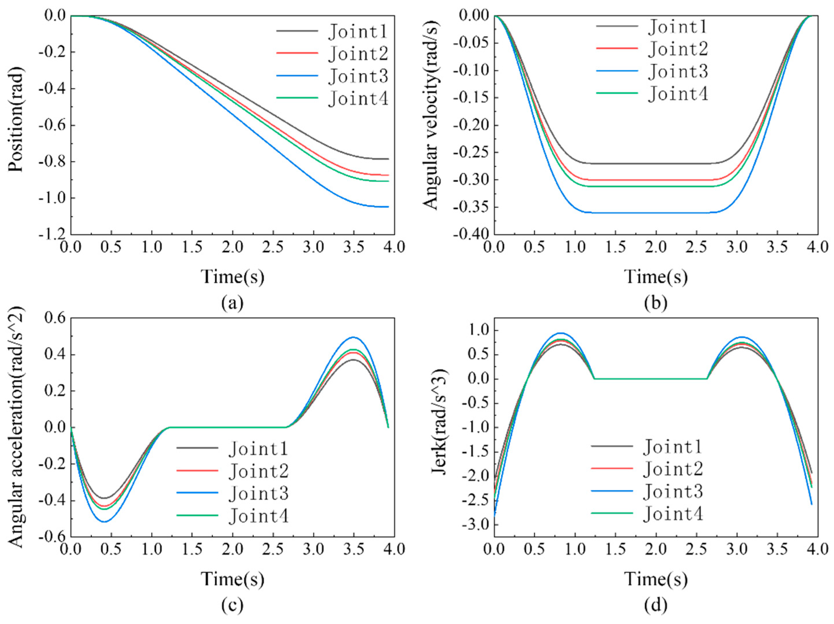
• To more closely resemble a human-like motion, a bounded jerk trajectory was constructed using the WOA, with a minimal running time as the optimization objective;
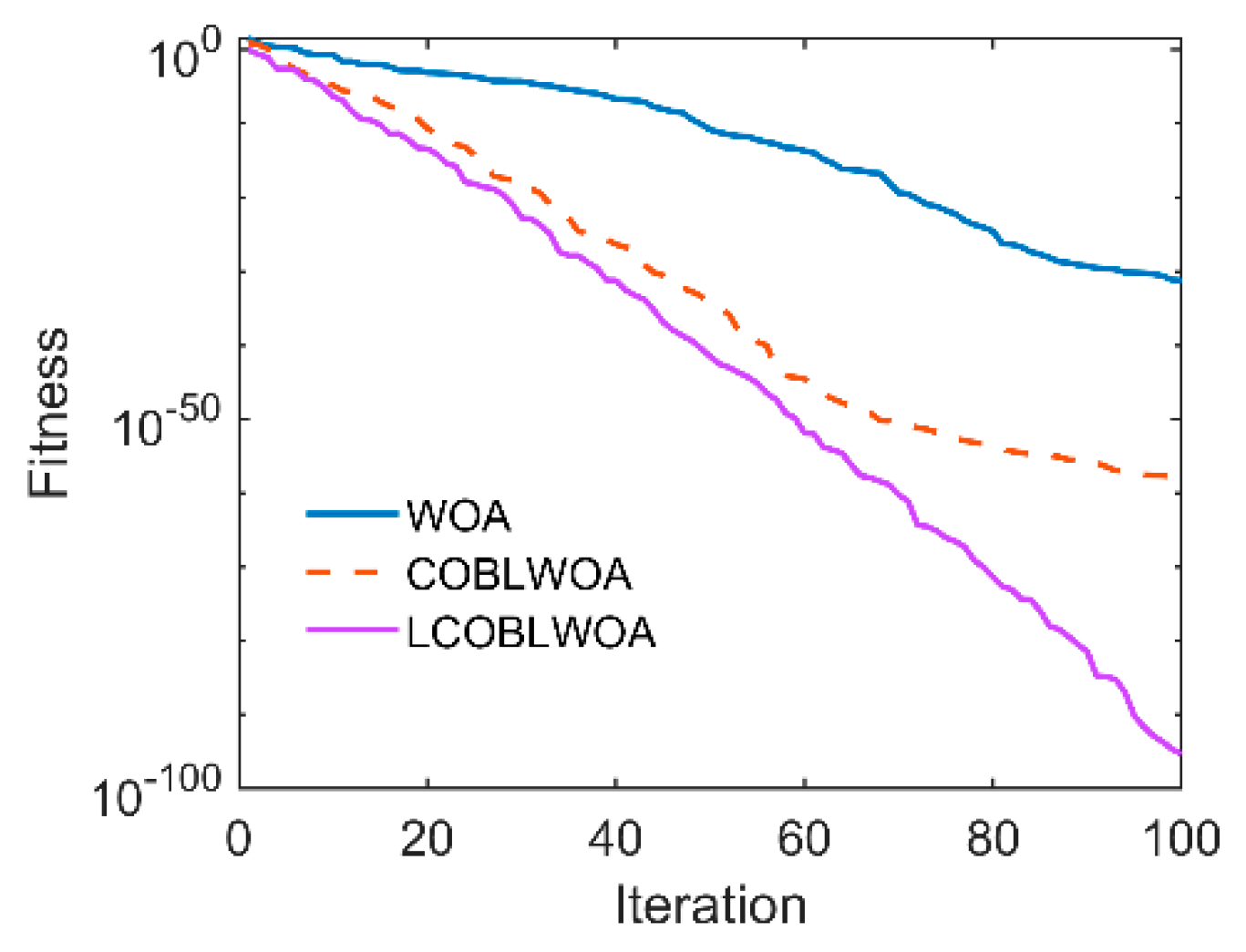
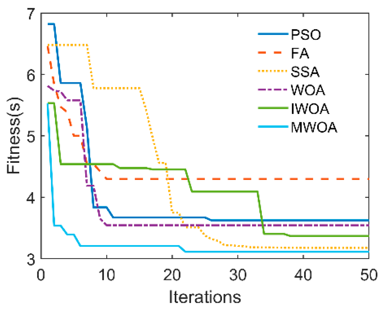
• To tackle the WOA’s shortage in search ability under complex constraints, three strategies were integrated into the proposed MWOA, and the resulting trajectories were compared to those obtained by the original WOA. A dual-population search with a novel communication mechanism to bypass local optimum was used. Mutation centroid opposition-based learning was used to improve the diversity of the population. An adaptive inertia weight mechanism was used to balance the WOA’s exploration and exploitation abilities;
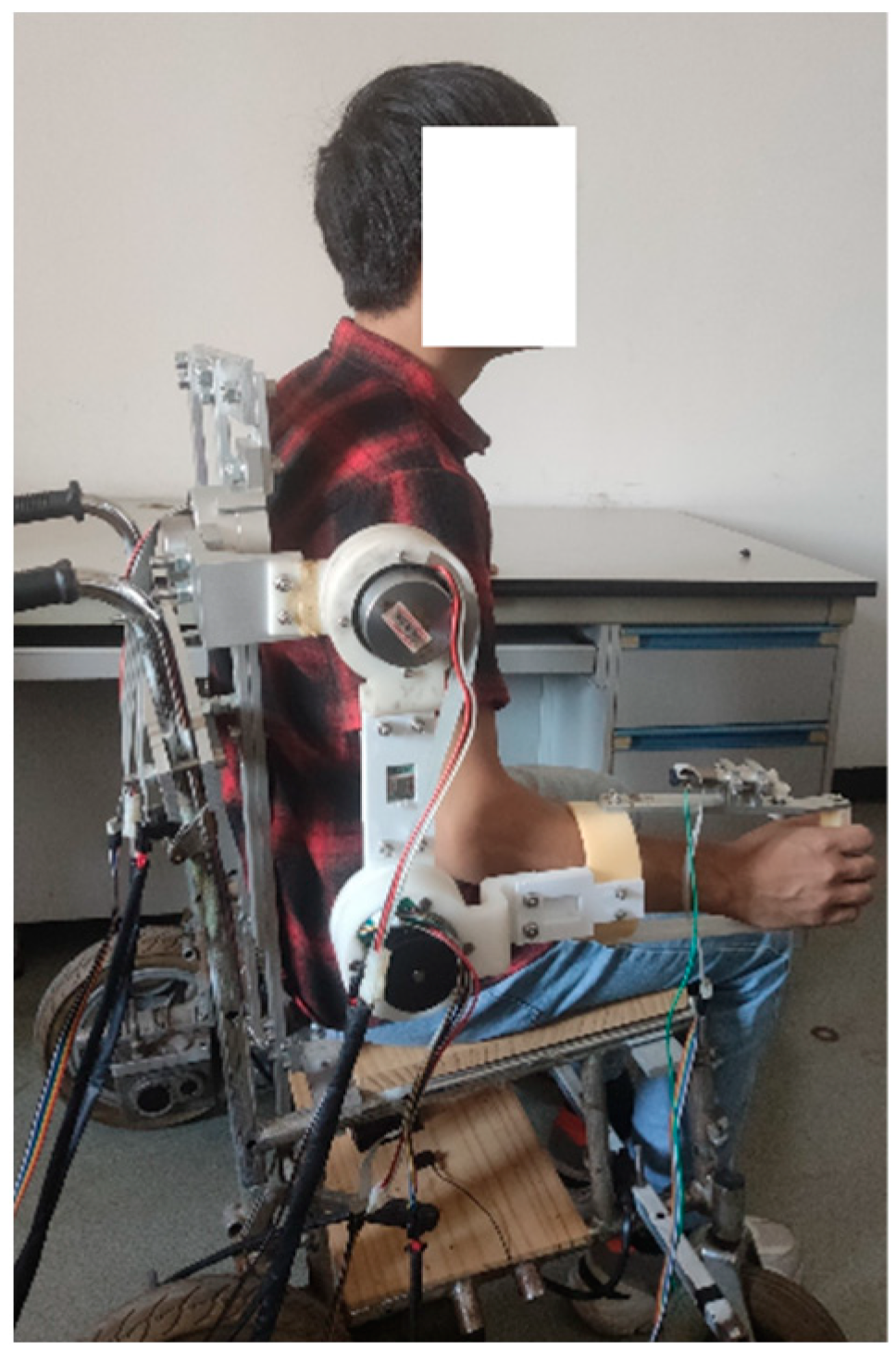
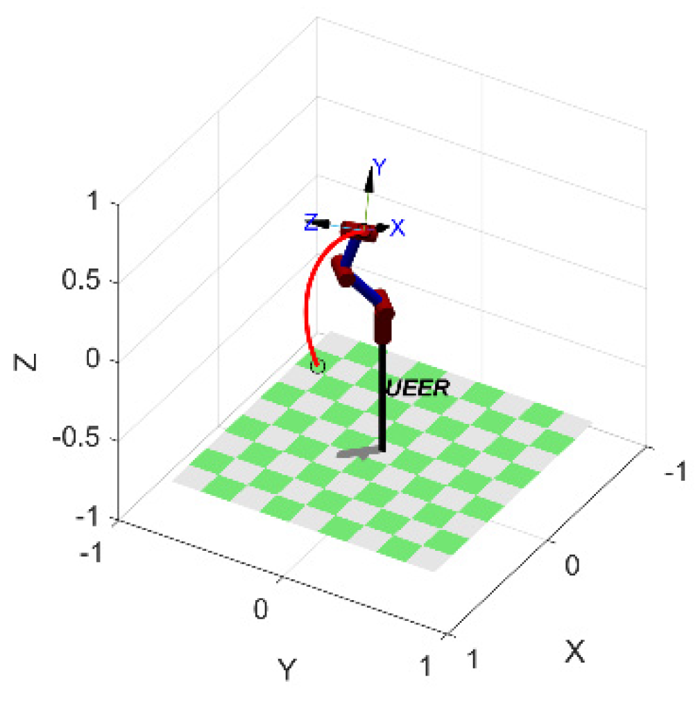
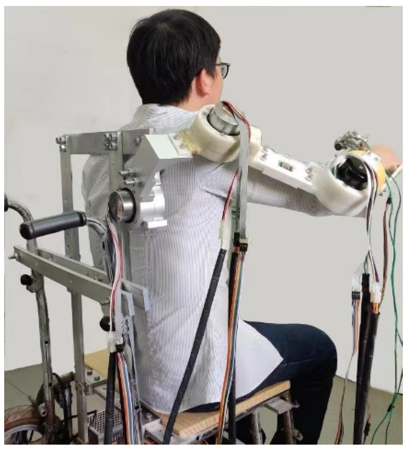
• Finally, a 4-DOF upper extremity exoskeleton rehabilitation (4-DOF UEER) robot was tested by simulation analysis and then validated on a healthy volunteer to mimic isokinetic rehabilitation training along the trajectory planned by the MWOA.

The organization of this paper is as follows: Section 2 describes the piecewise polynomial trajectory and the trajectory optimization problem. Section 3 briefly introduces the whale optimization algorithm, mainly describing the improvement in the whale optimization algorithm and the trajectory optimization based on this algorithm. Section 4 briefly introduces the 4-DOF UEER robot, simulation analysis and pilot experiment. The main conclusions are summarized in Section 5.

2. Piecewise Polynomial Trajectory Planning

2.1. Generation of a Preliminary Rehabilitation Trajectory by Piecewise Polynomial

Isokinetic training is characterized by maintaining a relatively uniform speed throughout the movement [14,34]. In addition, since the degrees of freedom in upper extremity exoskeleton rehabilitation robots correspond to those of a human’s upper limb, the contact between a robot and a patient is close during isokinetic rehabilitation. Moreover, due to the abnormal muscle tension present in hemiplegic patients, abrupt changes in the motion trajectory should be avoided to prevent secondary injury. With safety and effectiveness in mind, a piecewise polynomial trajectory containing a uniform velocity segment was used as a starting point for isokinetic training planning. Generally, lower-order polynomial trajectories are prone to impact, while higher-order polynomial trajectories are smoother but come at a higher computational cost. In order to ensure a continuous and smooth trajectory without impact, the fifth-order polynomial was selected for the acceleration and deceleration segments of the trajectory, and intermediate segment of the trajectory is linear (first-order polynomial). Equation (1) shows the piecewise polynomial trajectory. The 1st, 2nd, and 3rd segments represent the acceleration, uniform velocity, and deceleration phases, respectively. The corresponding symbols are described in

Table 1. Symbols used in the piecewise polynomial.

Symbols	Description
$i$	$i=1,2,\cdots ,n$, $n$$\mathrm{is} \mathrm{the} \mathrm{number} \mathrm{of} \mathrm{joints}, i$$\mathrm{is} \mathrm{the} i$th joint.
$p_{i1}\left(t\right)$$, p_{i2}\left(t\right)$$, p_{i3}\left(t\right)$	The 1st, 2nd, and 3rd segment of the trajectory, respectively.
$b_{i1j}$$, b_{i2j}$$, b_{i3j}$	$\mathrm{The} j$th coefficient of the 1st, 2nd, and 3rd segment of the trajectory, respectively.
${\tau }_{i1}$$,{\tau }_{i2}$$, {\tau }_{i3}$	Time corresponding to the 1st and 2nd transition points and the terminal point, respectively.

.

In Equation (1), the trajectory $p_i\left(t\right)$ is a time-dependent function, The angular velocity, angular acceleration, and jerk can be obtained by the first-order, second-order and third-order derivatives of $p_i\left(t\right)$ for time, respectively.

$$\begin{array}{c}\left\{\begin{array}{c}{p}_{i1}\left(t\right)=b_{i15}{t}^5+b_{i14}{t}^4+b_{i13}{t}^3+b_{i12}{t}^2+b_{i11}t+b_{i10},t\in [0,{\tau }_{i1}]\\ p_{i2}\left(t\right)=b_{i21}\left(t-{\tau }_{i1}\right)+b_{i20},t\in [{\tau }_{i1},{\tau }_{i2}]\\ p_{i3}\left(t\right)=b_{i35}{\left(t-{\tau }_{i2}\right)}^5+b_{i34}{\left(t-{\tau }_{i2}\right)}^4+b_{i33}{\left(t-{\tau }_{i2}\right)}^3+b_{i32}{\left(t-{\tau }_{i2}\right)}^2+\\ b_{i31}\left(t-{\tau }_{i2}\right)+b_{i30},t\in [{\tau }_{i1},{\tau }_{i2}]\\ \end{array}\right.\end{array}$$

(1)

If $t_{i1}$, $t_{i2}$, and $t_{i3}$ are the running time of the 1st, 2nd, and 3rd segments of the trajectory, respectively, then,${\tau }_{i1}=t_{i1}$, ${\tau }_{i2}=t_{i2}+{\tau }_{i1}$, and ${\tau }_{i3}=t_{i3}+{\tau }_{i2}$.

The range of motion of a patient’s joint is generally given by the physiotherapist to obtain the initial position ${\theta }_{\mathrm{i}0}$, and the terminal position ${\theta }_{if}$. The trajectory is continuous; thus, position, angular velocity, angular acceleration, and jerk are continuous at two transition points. To ensure safety, the angular velocity and angular acceleration at both positions are zero. This produces 14 equations than can be expressed in matrix form (Equation (2)):

$$TB=\theta$$

(2)

where $\theta ={\left[\mathrm{0,0},\mathrm{0,0},\mathrm{0,0},\mathrm{0,0},{\theta }_{if},\mathrm{0,0},{\theta }_{\mathrm{i}0},\mathrm{0,0}\right]}^T$, denoting the position vector of the joint. $T$ denotes the time parameter matrix, $T=\left[\begin{array}{ccc}{T}_{11}& T_{12}& \mathbf{0}\\ \mathbf{0}& T_{22}& T_{23}\\ T_{31}& T_{32}& T_{33}\end{array}\right]$, where $T_{11}=\left[\begin{array}{ccccc}{t}_{\mathrm{i}1}^5& t_{\mathrm{i}1}^4& t_{\mathrm{i}1}^3& t_{\mathrm{i}1}^2& t_{\mathrm{i}1}\\ 5t_{\mathrm{i}1}^4& 4t_{\mathrm{i}1}^3& 3t_{\mathrm{i}1}^2& 2t_{\mathrm{i}1}& 1\\ 20t_{\mathrm{i}1}^3& 12t_{\mathrm{i}1}^2& 6t_{\mathrm{i}1}& 2& 0\\ 60t_{\mathrm{i}1}^2& 24t_{i1}& 6& 0& 0\end{array}\right]$, $T_{12}=\left[\begin{array}{cccc}1& 0& -1& 0\\ 0& -1& 0& 0\\ 0& 0& 0& 0\\ 0& 0& 0& 0\end{array}\right]$, $T_{22}=\left[\begin{array}{cccc}0& t_{\mathrm{i}2}& 1& 0\\ 0& 1& 0& 0\\ 0& 0& 0& 0\\ 0& 0& 0& 0\\ 0& 0& 0& t_{\mathrm{i}3}^5\end{array}\right]$, $T_{23}=\left[\begin{array}{ccccc}0& 0& 0& 0& -1\\ 0& 0& 0& -1& 0\\ 0& 0& -2& 0& 0\\ 0& -6& 0& 0& 0\\ t_{\mathrm{i}3}^4& t_{\mathrm{i}3}^3& t_{\mathrm{i}3}^2& t_{\mathrm{i}3}& 1\end{array}\right]$, $T_{31}=\left[\begin{array}{ccccc}0& 0& 0& 0& 0\\ 0& 0& 0& 0& 0\\ 0& 0& 0& 0& 0\\ 0& 0& 0& 0& 1\\ 0& 0& 0& 2& 0\end{array}\right]$, $T_{32}=\left[\begin{array}{cccc}0& 0& 0& 5t_{\mathrm{i}3}^4\\ 0& 0& 0& 20t_{\mathrm{i}3}^3\\ 1& 0& 0& 0\\ 0& 0& 0& 0\\ 0& 0& 0& 0\end{array}\right]$, and $T_{33}=\left[\begin{array}{ccccc}4t_{\mathrm{i}3}^3& 3t_{\mathrm{i}3}^2& 2t_{\mathrm{i}3}& 1& 0\\ 12t_{\mathrm{i}3}^2& 6t_{\mathrm{i}3}& 2& 0& 0\\ 0& 0& 0& 0& 0\\ 0& 0& 0& 0& 0\\ 0& 0& 0& 0& 0\end{array}\right]$.

Coefficient matrix $B={\left[B_1,B_2,B_3\right]}^T$where $B_1=\left[b_{i15},b_{i14},b_{i13},b_{i12},b_{i11},b_{i10}\right]$, $B_2=\left[b_{i21},b_{i20}\right],$ and $B_3=\left[b_{i35},b_{i34},b_{i33},b_{i32},b_{i31},b_{i30}\right]$.

As mentioned above, the time parameter matrix $T$ can be obtained once $t=[t_1,t_2,t_3]$ is determined; then, the coefficient matrix $B$ can be calculated by Equation (3). Finally, the trajectory can be calculated by substituting B into Equation (1).

$$B=T^{-1}\theta$$

(3)

2.2. Description of the Trajectory Optimization Problem

Since polynomial functions cannot fully mimic natural human motion, optimization-based methods have been developed to generate human-like trajectories, most commonly the minimum jerk trajectory [35]. A commonly used alternative for trajectory planning is the bounded jerk method, of which Frisoli et al.’s [36] bounded jerk trajectory for robot-assisted stroke neurorehabilitation is a notable example. In addition to its resemblance to human movement, Chang et al. [34] have put forward the trajectory’s running time as a signific index for rehabilitation. In this regard, Qie et al. [37] used a genetic algorithm (GA) to generate a trajectory with minimum running time, effectively reducing motion time and improving rehabilitation effectiveness. Therefore, a bounded jerk trajectory was chosen in the present study to achieve a more human-like rehabilitation movement, and the total running time was taken as the optimization objective in order to improve rehabilitation effectiveness. The fitness function can be expressed:

$$f=\mathit{min}(t_{i1}+t_{i2}+t_{i3})$$

(4)

For safety reasons, angular velocity, angular acceleration, and jerk should be limited. Furthermore, to ensure effectiveness, a time constraint for the 2nd segment with the longest running time was added, expecting that rehabilitation produces its maximal effect in the uniform velocity segment. These constraints can be expressed as in Equation (5):

$$\left\{\begin{array}{c}{\dot{\theta }}_{imin}<\left|{\dot{\theta }}_{ij}\right|<{\dot{\theta }}_{imax}\\ \left|{\ddot{\theta }}_{ij}\right|<{\ddot{\theta }}_{imax}\\ \left|{\stackrel{⃛}{\theta }}_{ij}\right|<{\stackrel{⃛}{\theta }}_{imax}\\ \max \left(t_{i1},t_{i3}\right)<t_{i2}\end{array}\right.$$

(5)

where ${\dot{\theta }}_{ij}$, ${\ddot{\theta }}_{ij}$, and ${\stackrel{⃛}{\theta }}_{ij}$ represent angular velocity, angular acceleration, and jerk of the $i$th joint of the $j$th segment trajectory, respectively, ${\dot{\theta }}_{imin}$ and ${\dot{\theta }}_{imax}$ are the minimum and maximum angular velocity of the $i$th joint, respectively. ${\ddot{\theta }}_{imax}$ and ${\stackrel{⃛}{\theta }}_{imax}$ are the maximum angular acceleration and jerk of the $i$th joint, respectively. Note that the minimum angular velocity refers to the uniform velocity segment, which is necessary for adequate training intensity.

In case of violations to these constraints, a penalty was imposed using a penalty function described elsewhere [38]:

$$\left\{\begin{array}{c}{f}_{vj}=\left\{\begin{array}{cc}{\lambda }_{vj}& others\\ 0& {\dot{\theta }}_{imin}<\left|{\dot{\theta }}_{ij}\right|<{\dot{\theta }}_{imax}\end{array}\right.\\ f_{aj}=\left\{\begin{array}{cc}{\lambda }_{aj}& \left|{\ddot{\theta }}_{ij}\right|>{\ddot{\theta }}_{imax}\\ 0& others\end{array}\right.\\ f_{pj}=\left\{\begin{array}{cc}{\lambda }_{pj}& \left|{\stackrel{⃛}{\theta }}_{ij}\right|>{\stackrel{⃛}{\theta }}_{imax}\\ 0& others\end{array}\right.\\ f_{tj}=\left\{\begin{array}{cc}{\lambda }_{tj}& \mathit{max}(t_{i1},t_{i3})\ge t_{i2}\\ 0& others\end{array}\right.\end{array}\right.$$

(6)

where $f_{vj}$, $f_{aj}$, $f_{pj}$, and $f_{tj}$ represent the angular velocity, angular acceleration, jerk, and time penalty of the $j$th segment trajectory, respectively, and ${\lambda }_{vj}$, ${\lambda }_{aj}$, ${\lambda }_{pj}$, and ${\lambda }_{tj}$ are the angular velocity, angular acceleration, jerk, and time penalty weight of $j$th segment trajectory, respectively.

Therefore, the ultimate fitness function can be expressed in Equation (7) as:

$$f=\mathit{min}(\sum _{j=1}^3(t_{ij}+f_{vj}+f_{aj}+f_{pj}+f_{tj}))$$

(7)

Accordingly, as more constraints are violated, the fitness value increases and eventually the optimal trajectory is found.

3. Optimization Algorithm

3.1. Whale Optimization Algorithm

The whale optimization algorithm (WOA) is a meta-heuristic intelligent optimization algorithm proposed by Mirjalili [20] in 2016. This algorithm was inspired by the characteristic spiral foraging behavior of humpback whales known as the bubble-net hunting strategy. This algorithm consists of three main mathematical models, namely the encircling prey, bubble-net attacking method, and search for prey models.

3.1.1. Encircling Prey

This model assumes that the current optimal individual (the best search agent) is the target prey, and other particles (search agents) update their positions by approaching the optimal individual. The mathematical model is as follows:

$$\left\{\begin{array}{c}D=\left|C{X}^{\mathrm{*}}\left(k\right)-X\left(k\right)\right|\\ X\left(k+1\right)=X^{\mathrm{*}}\left(k\right)-AD\end{array}\right.$$

(8)

$$\left\{\begin{array}{c}A=2ar-a\\ C=2r\end{array}\right.$$

(9)

where $X$ is the position of particle, $X^{*}$ is the position of the optimal individual obtained so far, and $C$ denotes the swing factor. $\left|\right|$ is the absolute value, $r$ is a random number in [0, 1], $a$ is the convergence factor that is linearly reduced from 2 to 0 over the course of the iterations, and $k$ indicates the current iteration.

3.1.2. Bubble-Net Attacking Method (Exploitation Phase)

Humpback whales swim along a spiral path and spit bubbles, shrinking and encircling the prey simultaneously. To simulate this behavior, this algorithm assumes a probability of 50% of choosing either the shrinking encircling mechanism or the spiral updating position. The model is expressed in Equations (10) and (11):

$$\begin{array}{cc}X\left(k+1\right)=X^{\mathrm{*}}\left(k\right)-AD& if p<0.5\end{array}$$

(10)

$$\left\{\begin{array}{c}X\left(k+1\right)=D^{\prime }{e}^{bl}\cos \left(2\pi l\right)+X^{\mathrm{*}}\left(k\right) if p\ge 0.5\\ D^{\prime }=\left|X^{\mathrm{*}}\left(k\right)-X\left(k\right)\right|\end{array}\right.$$

(11)

where $p$ denotes probability and is a random number in [0, 1], $b$ is a constant that defines the shape of the spiral, and $l$ is a random number in [−1, 1].

3.1.3. Search for Prey (Exploration Phase)

This model allows particles to randomly search when $\left|A\right|\ge 1$, particles update their positions according to the randomly selected particle rather than the optimal individual. This model is shown in Equation (12):

$$X\left(k+1\right)=X_{rand}-A\left|C{X}_{rand}-X\left(k\right)\right|$$

(12)

where $X_{rand}$ represents a randomly selected particle.

3.2. Multistrategy Improved Whale Optimization Algorithm (MWOA)

Despite its good optimization performance, the reliability of the WOA is limited under complex constrains. To enable the WOA’s reliability for trajectory optimization under the above-mentioned constraints, a multistrategy improved whale optimization algorithm (MWOA) was designed. The new MWOA was aimed at improving the diversity of the population and balancing the algorithm’s exploration and exploitation performance to prevent it from prematurely falling into a local optimum.

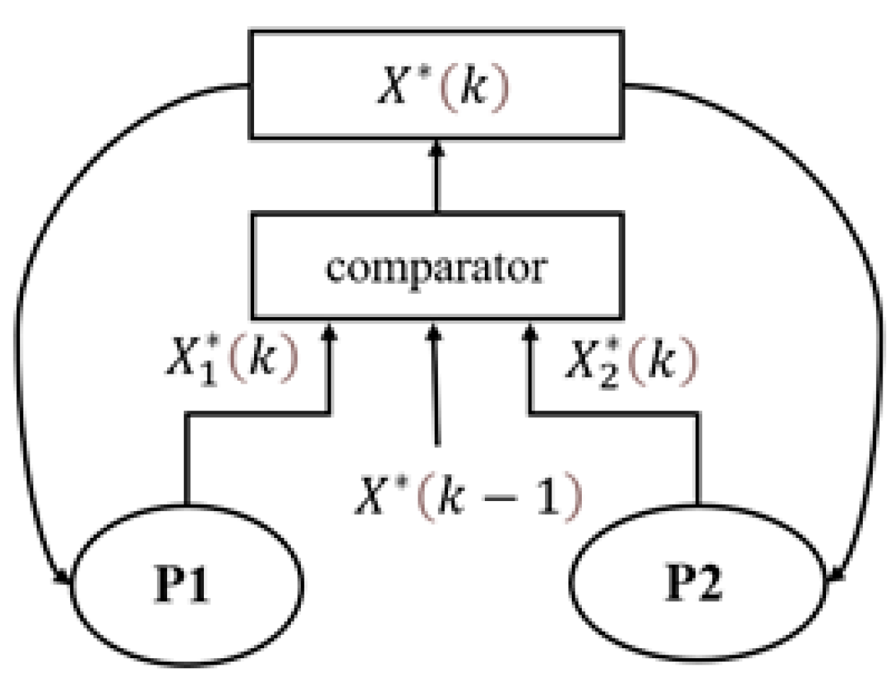
3.2.1. Dual-Population Search

To initialize the population, the WOA uses a random method that cannot guarantee the diversity of the initial population. In addition, a single population lacks a mechanism to communicate with external information, making it difficult to escape a local optimum position once it has fallen into one. The dual-population search is equivalent to initializing different populations twice and improves the diversity of the initial population to a certain extent. Moreover, dual-population constantly communicate search information in a parallel search process so as to avoid falling into a local optimum.

However, if two subpopulations $P_1$ and $P_2$ search their personal optimal individual $X_1^{*}$ and $X_2^{*}$ in a given iteration, inappropriate communication between the two subpopulations can be counterproductive. To tackle this issue, a new communication mechanism is proposed in the current study, as follows:

$$V\left(k\right)=V\left(k-1\right)+r_1\ast \left(H\left(k\right)-L\left(k\right)\right)+r_2\ast \left(H\left(k\right)-X^{\mathrm{*}}\left(k-1\right)\right),(k\ge 2)$$

(13)

$$X^{\mathrm{*}}\left(k\right)=r_3\ast X^{\mathrm{*}}\left(k-1\right)+V\left(k\right)$$

(14)

where $H\left(k\right)$ and $L\left(k\right)$ denote the better and the worse personal optimal individual between $X_1^{*}$ and $X_2^{*}$ in the $k$th iteration, respectively, and $X^{*}\left(k\right)$ represents the position of the global optimal individual in the $k$th iteration. As determined by $X^{*}\left(1\right)$ = $H\left(1\right)$, the better personal optimal individual is regarded as the global optimal individual in the 1st iteration. $V\left(k\right)$ is the variation in the $k$th iteration, and $r_1$, $r_2$, and $r_3$ are random numbers in [0, 1].

Through this communication mechanism, beginning from the 2nd iteration, the global optimal individual is determined by the global optimal individual of the last iteration and the variation in the current iteration. The variation consists of three parts: the first is the variation in the last iteration, the second is the difference between the personal optimal individuals of the two subpopulations in the current iteration, and the third is the difference between the current iteration’s better personal optimal individual and the global optimal individual of the last iteration. This means that the global optimal individual combines the search capabilities of the two subpopulations in the current iteration and the search experience obtained by the entire population, as opposed to taking only the optimal individual of a certain subpopulation. Furthermore, even if a subpopulation falls into a local optimum, it can escape through this communication mechanism, effectively reducing the probability of falling into local optima. Once a certain dimension of $X^{*}\left(k\right)$ exceeds the search space boundary, it is replaced by the corresponding dimension of $H\left(k\right)$. This newly proposed communication mechanism is represented in Figure 1.

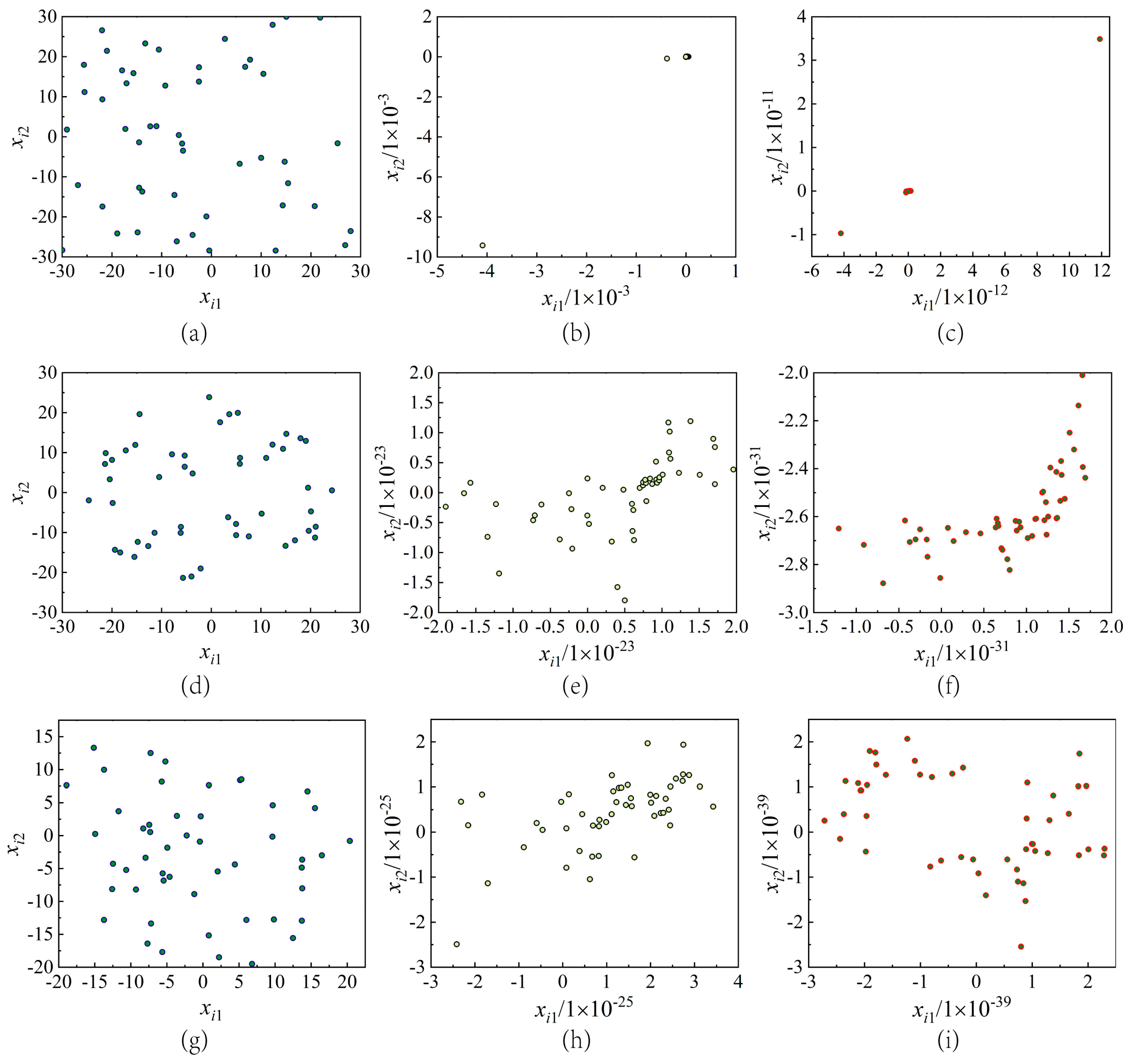
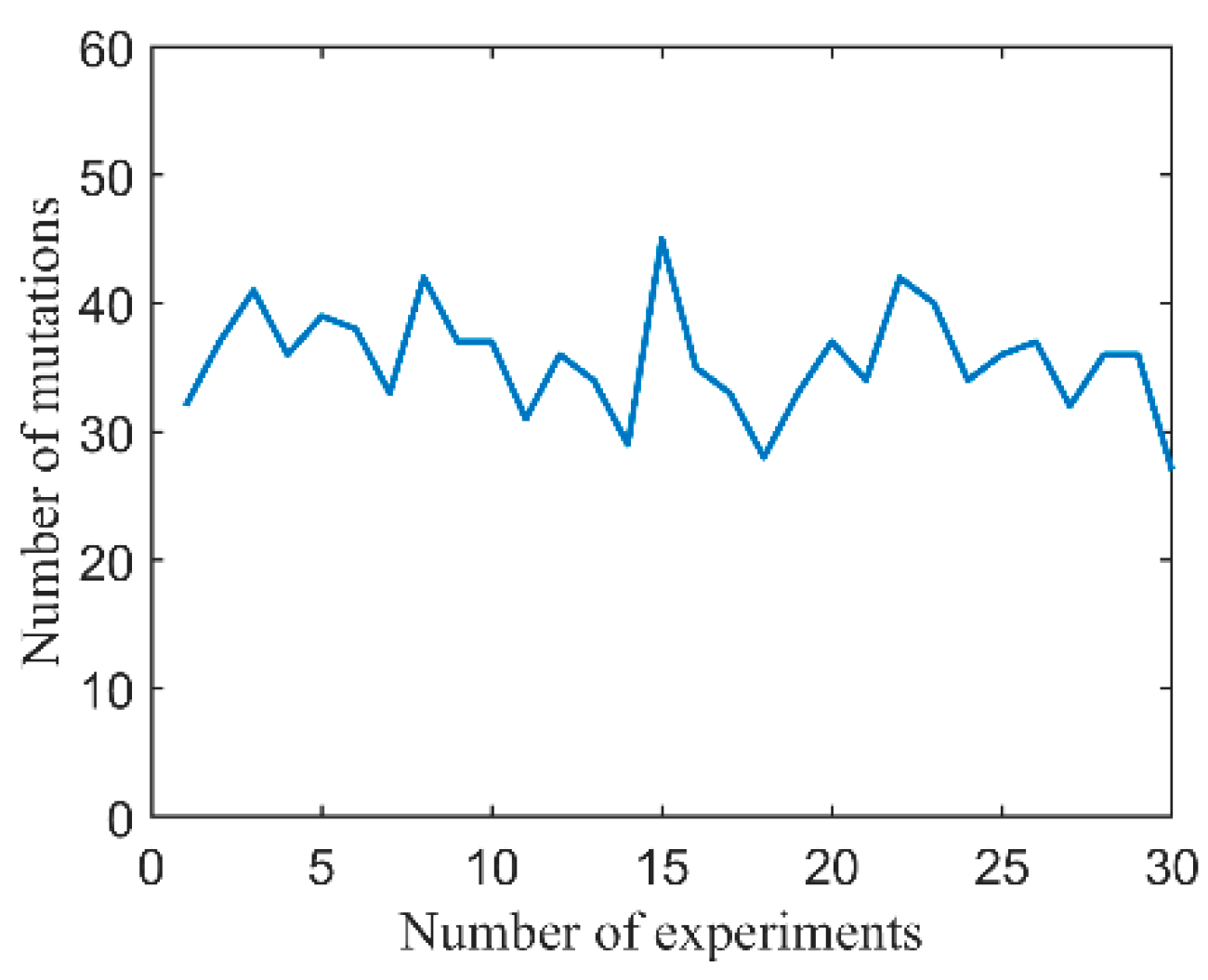
3.2.2. Mutation Centroid Opposition-Based Learning

In centroid opposition-based learning (COBL), the centroid of the current population is taken as reference point to calculate the opposite population. The two populations are then combined into a single population and several particles with the highest fitness are selected to ultimately form a population.

Assume that population $P=(X_1;\cdots ;X_N)$ is composed of $N$ particles with $D$ dimensional search space, then the centroid of the population can be defined as follows:

$$M=\frac{X_1+\cdots +X_N}{N}$$

(15)

Each particle $X_i=(x_{i1},x_{i2},\cdots ,x_{ij})$, where $x_{ij}\in \left[lb,ub\right]$. Then:

$$M_j=\frac{{\sum }_{i=1}^N{x}_{ij}}{N},j=1,\cdots ,D$$

(16)

where $lb$ and $ub$ denote the lower and upper boundary of the search space, respectively.

Having defined the centroid of the population as $M$, the opposite particle, ${\overline{X}}_i$, of particle $X_i$ can be calculated as follows:

$${\overline{X}}_i=2\times M-X_i$$

(17)

Particles beyond the boundary are recalculated according to Equation (18):

$${\overline{x}}_{ij}=\left\{\begin{array}{cc}lb+r\times \left(ub-lb\right)& {\overline{x}}_{ij}<lb\\ ub-r\times \left(ub-lb\right)& {\overline{x}}_{ij}>ub\end{array}\right.$$

(18)

where $r$ is a random number in [0, 1].

For convergence, the WOA performs local exploitation during the middle and later stages. As particles gradually gather around the optimal individual, the centroid changes very little, which in turn renders COBL ineffective to preserve the diversity of the population. For this reason, a mutation operation is implemented to help the centroid jump out of the current gathering, whereby all particles are able to change in response to the change of reference point, thus improving the diversity of the population. The centroid mutation operation is expressed by Equation (19):

$$M^{\prime }=M\times \left(1+\gamma \right)$$

(19)

where $\gamma$ indicates the mutation operator and $M^{\prime }$ is the centroid after mutating.

Since it cannot be guaranteed that the position of the centroid will improve after mutation, the greedy strategy is adopted to compare the fitness of the centroid before and after mutating. When the fitness of the centroid is better after mutation, the centroid is then updated to $M\prime$, otherwise the centroid remains unchanged.

Among the many available mutation operation methods, the Cauchy mutation and the Levy mutation have been shown to be the most effective, especially in comparison to the Gaussian mutation [39]. Therefore, the present paper employed the Cauchy and Levy mutations for centroid mutation.

• Cauchy Mutation

This is a random mutation operation based on the Cauchy distribution. Zhao [40] demonstrated the effectiveness of the Cauchy mutation in improving the diversity of the population when applied to the grasshopper optimization algorithm (GOA). The standard Cauchy distribution is shown in Equation (20):

$$f_c\left(x\right)=\frac{1}{\pi \left(1+x^2\right)},-\mathrm{\infty }<x<\mathrm{\infty }$$

(20)

The standard Cauchy distribution peaks at zero, it is lower in the middle and longer at both ends. This long-tailed distribution allows the centroid a higher probability of jumping to a better position that may significantly improve the diversity of the population. The Cauchy mutation is given in Equation (21):

$$Cauchy\left(\mathrm{0,1}\right)=\mathit{tan}\left[\left(\delta -0.5\right)\pi \right]$$

(21)

where $\delta \in \left(\mathrm{0,1}\right)$.

2.

Levy mutation

The Levy flight is a process of random walking, and its walking step size meets the heavy-tailed distribution [27]. The Levy mutation is described as follows:

$$L\left(\beta \right)=\frac{\mu \sigma }{{\left|v\right|}^{\frac{1}{\beta }}},0<\beta \le 2$$

(22)

where $\mu$ and $v$ belong to the standard normal distribution, and $\sigma$ is given by:

$$\sigma ={\left[\frac{\Gamma (1+\beta )\mathit{sin}(\frac{\pi \beta }{2})}{\Gamma \left(\frac{1+\beta }{2}\right)\beta 2^{\left(\frac{\beta -1}{2}\right)}}\right]}^{\frac{1}{\beta }}$$

(23)

where $\Gamma (·)$ is the standard gamma function and $\beta$ = 1.5.

The Levy mutation is characterized by predominantly small steps and occasional large steps, i.e., small or large centroid changes, which can improve the diversity of the population.

Both mutations are each applied to one of the two subpopulations, centroid mutation is ultimately expressed by Equation (24):

$$\left\{\begin{array}{c}{M}^{\prime }=M\times \left(1+Cauchy\right) or\\ M^{\prime }=M\times \left(1+L\left(\beta \right)\right)\end{array}\right.$$

(24)

To verify the effect of mutation centroid opposition-based learning, the Levy mutation was applied to the WOA (referred to as the Levy mutation centroid opposition-based learning whale optimization algorithm, LCOBLWOA) and compared to the centroid opposition-based learning whale optimization algorithm (COBLWOA) and the WOA alone. For these comparisons, the standard benchmark function Sphere, whose theoretical optimal value is zero, was taken as an example, and the population distribution was analyzed. The search dimension was set to $D$ = 2 in order to display the distribution of the population more intuitively. The remaining parameters were as follows: $lb$ = −30, $ub$ = 30, $N$ = 30, and the maximum iteration was 100. The 1st, 60th, and 84th iterations (the latter two randomly selected) were chosen to represent population distribution at the initial, middle, and later iterations, respectively.

The results are shown in Figure 2. It illustrates the population distributions obtained by the WOA, COBLWOA, and LCOBLWOA during different iterations. Figure 2a–c shows the population distribution obtained by the WOA at the 1st, 60th, and 84th iteration, respectively. As shown, the population was uniformly distributed in the initial iteration and the diversity of the population was abundant. In the 60th and 84th iterations, however, the population nearly gathered around three points, indicating a sharp decline in the diversity of the population. Figure 2d–f shows the population distributions of the COBLWOA. With this algorithm, the population remained uniformly distributed in the initial and middle iterations, but by the 84th iteration, the bulk of the population was distributed in an arc at the lower right. This indicates that, despite being conducive to the diversity of the population improvements throughout early to middle iterations, the COBL could not prevent the decline of diversity in later stages. Finally, Figure 2g–i shows the population distributions obtained by the LCOBLWOA. Over all the iterations analyzed, LCOBLWOA resulted in a uniformly distributed population, indicating abundant diversity across all iterations and confirming the effectiveness of the Levy mutation centroid opposition-based learning (LCOBL) to improve the diversity of the population.

Importantly, all three algorithms had different search boundaries even in the same iteration. For instance, in the 60th iteration, the WOA search boundary was on the magnitude of $1\times {10}^{-3}$, while the COBLWOA and the LCOBLWOA were on the magnitude of $1\times {10}^{-23}$ and $1\times {10}^{-25}$, respectively. The gap was greater in the 84th iteration, indicating that the three algorithms had different convergence speeds and convergence accuracies. This was confirmed upon inspection of the convergence curves (Figure 3), which also revealed that the LCOBLWOA had the fastest convergence speed and the highest convergence accuracy. To characterize the LCOBLWOA’s mutation trends, a set of 30 random experiments was run (Figure 4). The average number of mutations was 35.5667, with a standard deviation of 4.1413. This indicates that mutations in the LCOBLWOA occur in a relatively stable fashion. Additionally, experiments with the Cauchy mutation centroid opposition-based learning whale optimization algorithm were implemented with similar results. Taken together, mutation centroid opposition-based learning effectively improved the diversity of the population across all iterations and enhanced the search performance of the WOA.

3.2.3. Adaptive Inertia Weight

In the original WOA, particles update their positions without regard to the corresponding inertia weight. Since appropriate inertia weight can improve convergence accuracy, the present work introduced inertia weight to adaptively adjust the updated position. Inertia weight can be expressed as follows:

$$\omega ={\omega }_{max}-\left({\omega }_{max}-{\omega }_{min}\right)\left(\left(\frac{2\ast iter}{max\_iter}\right)-{\left(\frac{iter}{max\_iter}\right)}^2\right)$$

(25)

where ${\omega }_{max}$ and ${\omega }_{min}$ are the maximum and minimum adaptive inertia weights, respectively, $max\_iter$ indicates the maximum iteration, and $iter$ denotes the current iteration.

Adaptive inertia weight, $\omega$, decreases smoothly throughout iterations; it is larger during the early iterations and becomes smaller at later iterations, which improves the algorithm’s global exploration capability at the beginning and favors its local exploitation capability at a later stage. The improved WOA is thus expressed as:

$$X\left(k+1\right)=\omega X^{\mathrm{*}}\left(k\right)-AD$$

(26)

$$X\left(k+1\right)=D^{\prime }{e}^{bl}\cos \left(2\pi l\right)+\omega X^{\mathrm{*}}\left(k\right)$$

(27)

$$X\left(k+1\right)=\omega X_{rand}-A\left|C{X}_{rand}-X\left(k\right)\right|$$

(28)

The pseudo-code for the MWOA is also included in Algorithm 1.

Algorithm 1: Pseudo-code of MWOA algorithm.

1: $\mathrm{Initialize} \mathrm{two} \mathrm{subpopulations} P_1$$\mathrm{and} P_2$$, \mathrm{each} \mathrm{subpopulation} \mathrm{of} \mathrm{size} n_1$ and $n_2$, respectively.

2: $\mathrm{while} 1 (iter$ < $\mathrm{m}\mathrm{a}\mathrm{x}\_iter$) do

3:  $\mathrm{Use} \mathrm{Equation} \left(16\right) \mathrm{to} \mathrm{calculate} \mathrm{the} \mathrm{centroid} \mathrm{of} P_1$$\mathrm{and} P_2$$\mathrm{as} M_1$, $M_2$

4:  Levy $\mathrm{mutation} \mathrm{operator} \mathrm{for} \mathrm{centroid} M_1$$\mathrm{by} \mathrm{using} \mathrm{Equation} \left(24\right) \mathrm{and} \mathrm{create} L\_M_1$

5:     $\mathrm{if} \mathrm{f} (L\_M_1$$) < \mathrm{f} (M_1$$) // f(·)$ is fitness function

6:     $M_1^{\prime }\leftarrow L\_M_1$$//M_1^{\prime }$$\mathrm{denotes} \mathrm{centroid} \mathrm{of} P_1$ after mutating

7:   else

8:       $M_1^{\prime }\leftarrow M_1$

9:     end if

10:   In $P_1$$, \mathrm{use} \mathrm{Equations} (17) \mathrm{and} (18) \mathrm{calculate} \mathrm{opposite} \mathrm{subpopulation} \stackrel{-}{P_1}$

11:   $C\_P_1\leftarrow P_1\cup \stackrel{-}{P_1}$$, \mathrm{calculate} \mathrm{each} \mathrm{particle} \mathrm{fitness} \mathrm{of} C\_P_1$.

12:  $\mathrm{Sort} \mathrm{and} \mathrm{select} n_1$$\mathrm{fittest} \mathrm{individuals} \mathrm{from} \mathrm{the} C\_P_1$$\mathrm{to} \mathrm{replace} P_1$

13:  $\mathrm{Calculate} \mathrm{and} \mathrm{obtain} \mathrm{optimal} \mathrm{individual} X_1^{*}$$\mathrm{of} P_1$ 14:  Cauchy $\mathrm{mutation} \mathrm{operator} \mathrm{for} \mathrm{centroid} M_2$$\mathrm{by} \mathrm{using} \mathrm{Equation} \left(24\right) \mathrm{and} \mathrm{create} C\_M_2$

15:  $\mathrm{Similar} \mathrm{to} \mathrm{steps} 5–9, \mathrm{calculate} \mathrm{centroid} M_2^{\prime }$$\mathrm{of} P_2$

16:  $\mathrm{In} P_2$$, \mathrm{use} \mathrm{Equations} (17) \mathrm{and} (18) \mathrm{calculate} \mathrm{opposite} \mathrm{subpopulation} \stackrel{-}{P_2}$

17:   $C\_P_2\leftarrow P_2\cup \stackrel{-}{P_2}$$, \mathrm{calculate} \mathrm{each} \mathrm{particle} \mathrm{fitness} \mathrm{of} C\_P_2$

18:  $\mathrm{Sort} \mathrm{and} \mathrm{select} n_2$$\mathrm{fittest} \mathrm{individuals} \mathrm{from} \mathrm{the} C\_P_2$$\mathrm{to} \mathrm{replace} P_2$

19:  $\mathrm{Calculate} \mathrm{and} \mathrm{obtain} \mathrm{optimal} \mathrm{individual} X_2^{*}$$\mathrm{of} P_2$

20:  $\mathrm{Calculate} \mathrm{the} \mathrm{global} \mathrm{optimum} X^{*}$ by the new communication mechanism

21:  $\mathrm{while} 2 (iter$$\ge$ 2) do

22:     $\mathrm{Use} \mathrm{Equations} (13) \mathrm{and} (14) \mathrm{to} \mathrm{calculate} \mathrm{the} \mathrm{global} \mathrm{optimal} \mathrm{individual} X^{*}$

23:   end while 2

24:  $X_1^{*}\leftarrow X^{*}$; $X_2^{*}\leftarrow X^{*}$

25: $\mathrm{Update} \mathrm{parameters} \omega$$, a$

26:  $\mathrm{for} i=1:n_1$

27:    $\mathrm{update} \mathrm{parameters} A$$, C$$, l$$, p$

28:    $\mathrm{update} P_1$ using Equations (26)–(28), calculate the fitness of each particle

29:  end for

30:  $\mathrm{for} j=1:n_2$

31:   $\mathrm{update} \mathrm{parameters} A$$, C$$, l$$, p$

32:    $\mathrm{update} P_2$ using Equations (26)–(28), calculate the fitness of each particle

33:  end for

34: $\mathrm{Update} X^{*}$ if there is a better solution

35: $iter$ = $iter$ + 1

36: end while 1

37: return $X^{*}$

3.2.4. Trajectory Planning Process Based on the MWOA

The trajectory planning process using the MWOA comprises the following steps:

Step 1: Determine the initial and terminal position and constraints, randomly initialize two subpopulations $P_1$ and $P_2$, and with each particle expressing as $X_i=(t_{i1},t_{i2},t_{i3})$;

Step 2: Calculate the fitness of each particle in both subpopulations and update both subpopulations through the mutation centroid opposition-based learning method;

Step 3: Calculate the global optimal individual, $X^{*}$, through the new communication mechanism;

Step 4: Update $\omega$ and WOA parameters, update the position of $P_1$ and $P_2$ according to Equations (26)–(28) independently, and update $X^{*}$ if there is a better solution;

Step 5: Determine whether the iteration is terminated. If it is satisfied, output $X^{*}$, otherwise, return to Step 2;

Step 6: Substitute $X^{*}$ into Equation (3) to calculate coefficient matrix $B$, then substitute $B$ into Equation (1) to output the global optimal trajectory.

4. Simulation Analysis and Pilot Experiment

4.1. 4-DOF Upper Extremity Exoskeleton Rehabilitation Robot

The 4-DOF upper extremity exoskeleton rehabilitation (4-DOF UEER) robot used in this paper is illustrated in Figure 5. It consists of shoulder, elbow, and wrist components, which correspond to the joints found in human upper limbs. Joints 1 and 2 of the 4-DOF UEER robot are designed on the shoulder, where joint 1 performs abduction and adduction movements and joint 2 executes flexion and extension movements. Joints 3 and 4 mimic the elbow and wrist, respectively, and both perform flexion and extension movements. Together, the four joints, driven by servo motors, can assist a human patient to complete most upper limb movements. The positions and angular velocity of each joint could be obtained through embedded angle sensors and encoders. For the present work, the 4-DOF UEER robot was installed on a movable wheelchair, and it is thus freely mobile.

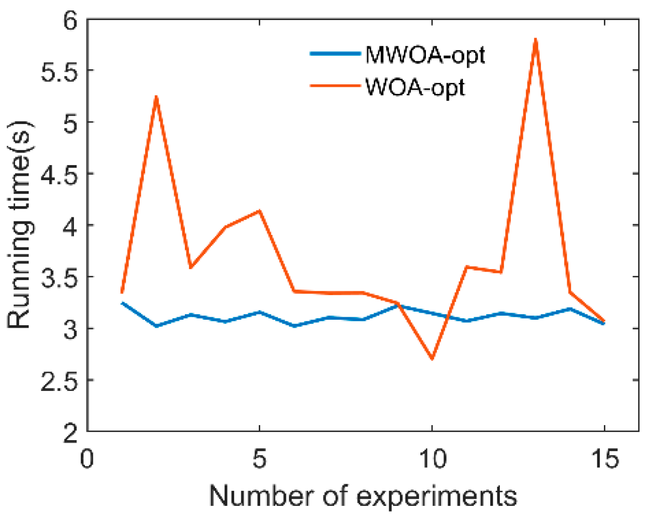
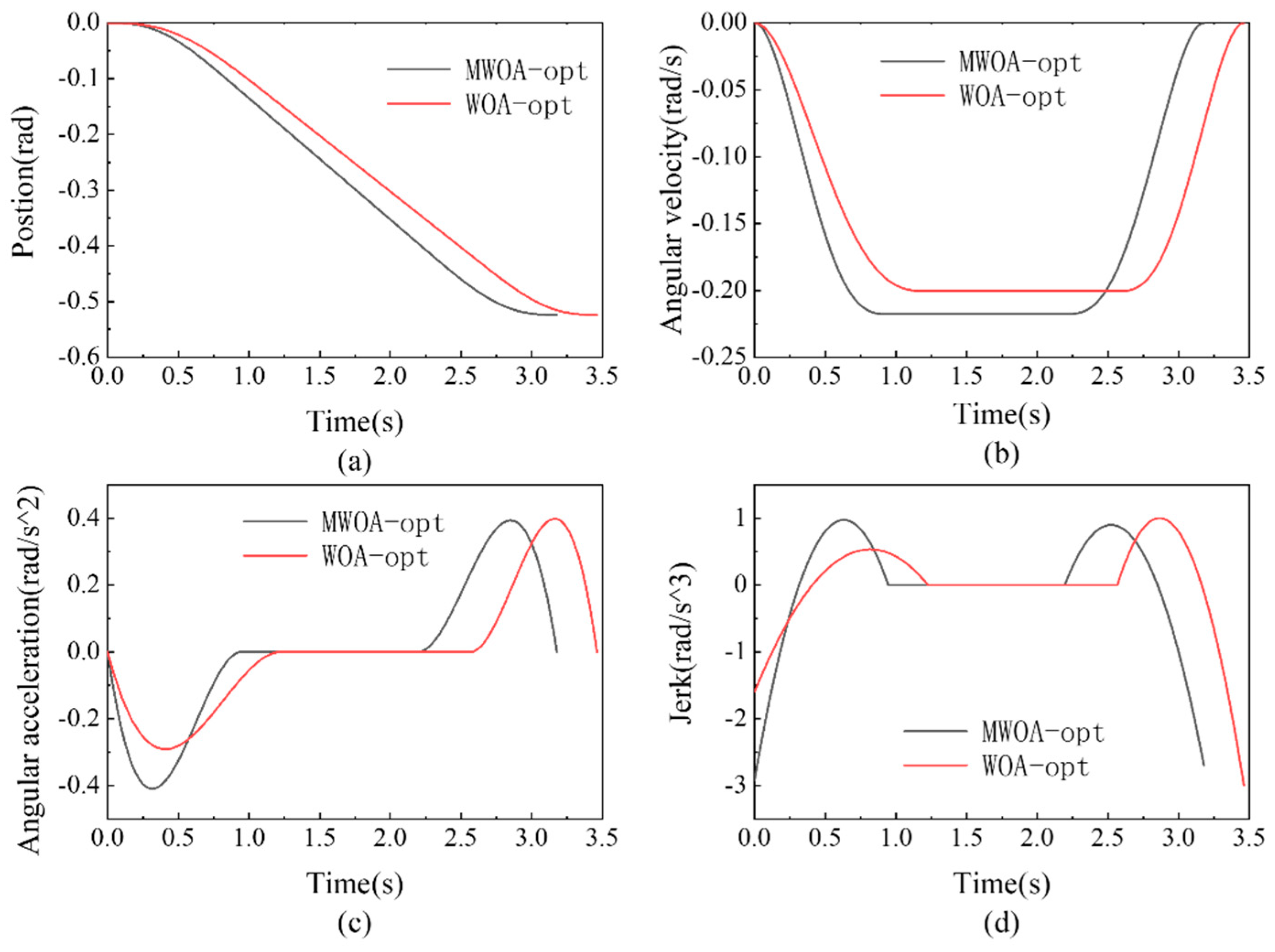
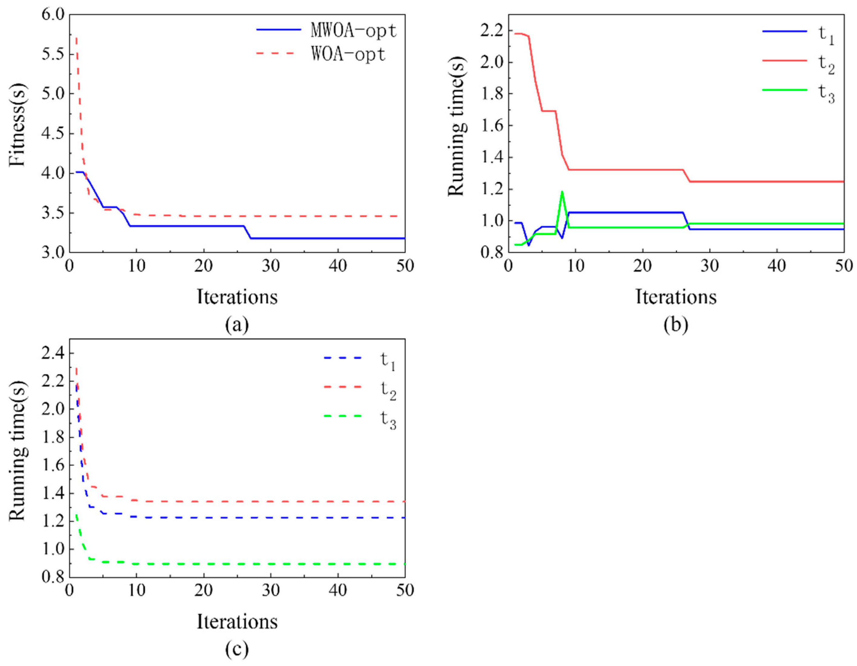
4.2. Single Joint Trajectory Planning Experiment

According to rehabilitation theory, the recovery of upper limb movement and function of stroke patients should start with rehabilitation of a single joint and gradually build up to multi-joint rehabilitation. For this reason, a trajectory was first planned for a single joint. The MWOA and the WOA were used to optimize the trajectory, assuming that the initial position ${\theta }_0$ = 0 and the terminal position ${\theta }_f$ = 0.5236 rad. Partial constraint values were obtained from the literature [14], the constraints were as follows: ${\dot{\theta }}_{imax}=0.5236 \mathrm{r}\mathrm{a}\mathrm{d}/\mathrm{s}$, ${\dot{\theta }}_{imin}=0.0873 \mathrm{r}\mathrm{a}\mathrm{d}/\mathrm{s}$, ${\ddot{\theta }}_{imax}=0.5236 \mathrm{r}\mathrm{a}\mathrm{d}/{\mathrm{s}}^2$, and ${\stackrel{⃛}{\theta }}_{imax}=3 \mathrm{r}\mathrm{a}\mathrm{d}/{\mathrm{s}}^3$. Common parameters were set as follows: ${\lambda }_{vj}={\lambda }_{aj}={\lambda }_{pj}={\lambda }_{tj}$ = 40 (the weights of all constraints were set to the same value since they were considered equally important), $max\_iter$ = 50, $lb=0.5$ s, $ub$ = 7 s, and $D=3$. The newly set experimental parameters are summarized in

Table 2. Experimental parameters.

Algorithm	$\mathbf{Population} \mathbf{Size} \mathit{N}$	$\mathit{\omega }$
WOA	30
MWOA	$P_1$$n_1$= 16 $P_2$$n_2$ = 14	${\omega }_{max}$ = 0.9 ${\omega }_{min}$ = 0.3

.

Given the randomness of the algorithms, 15 experiments were performed. As shown in Figure 6, the total running time of the trajectory optimized by the MWOA was lower than that of the WOA, with the exception the 10th experiment. Since the trajectory optimized by the WOA in the 10th experiment violated the time constraint, it was considered that no feasible solution could be found in this experiment. This also suggests that the WOA may be unable to find a feasible solution under complex constraints, which supports the notion that the WOA needs further improvement. Excluding data from the 10th experiment, the running time was 17.5670% shorter for the MWOA compared to the WOA, with an average running time of 3.1130 s and 3.7764 s, respectively, and a standard deviation of 0.0714 and 0.7967, respectively. These results confirmed that the MWOA has higher convergence accuracy and more stability than the WOA.

Experimental trajectories were randomly selected for further inspection (Figure 7). All trajectories were smooth and continuous, with the 2nd segment maintaining uniform velocity and the 1st and 3rd segments lacking sudden changes in angular velocity or angular acceleration or a continuous and bounded jerk curve, and all constraints were satisfied. In particular, the trajectory optimized by MWOA had a similar running time both in the 1st and 3rd segments, the jerk was close to the maximum value, and the angular velocity and angular acceleration were greater than the trajectory optimized by the WOA. In comparison, the running time of the 1st segment optimized by WOA was longer than its 3rd segment, the jerk approached the maximum value in the 3rd segment, and the angular velocity and angular acceleration were also larger than those for the 1st segment. This shows that the MWOA optimized a trajectory with better symmetry than the WOA.

To visualize the trajectory optimization process of both algorithms, convergence curves were plotted and are shown in Figure 8. The WOA converged at the 7th iteration, while the MWOA did not converge until the 27th iteration, which indicated that the WOA had a higher convergence speed. However, importantly, the WOA only searched for the local optimal solution, while the MWOA searched for a better solution. Figure 8b,c shows the convergence curves of running time for each trajectory segment. The running time of the 2nd segment was the longest and evidently satisfied the time constraints of the trajectory.

The above results confirmed that the MWOA successfully achieved a higher convergence accuracy and robustness than the WOA. Moreover, only the WOA failed to find a feasible solution in some instances, whereas the MWOA was always capable of finding a feasible solution, which further highlights the feasibility and reliability of the MWOA. These improvements were made possible by the different strategies integrated into the WOA. First, the dual-population search strategy improved the diversity of the initial population, and when used in tandem with the mutation centroid opposition-based learning strategy, which improved the diversity of the population throughout the entire iterative process, it allowed for a wider search space. In addition, the new communication mechanism proposed in this paper that allowed the two subpopulations to continuously communicate their search information to avoid premature convergence. Finally, the adaptive inertia weight parameter balanced the local exploitation and global exploration capabilities and improved the convergence accuracy of the algorithm.

The MWOA was also compared to other famous optimization algorithms, namely the particle swarm optimization algorithm (PSO) [41], the firefly algorithm (FA) [42], the salp swarm algorithm (SSA) [43], and the improved whale optimization algorithm (IWOA) [21]. Each algorithm was run in 15 randomized experiments under the same experimental conditions, taking other parameters from their original reference. The index $E_m$ [17] was used to evaluate optimization performance; the smaller the $E_m$ value, the better the optimization performance. In addition, the number of times an algorithm failed to find a feasible solution was also used to evaluate optimization performance. Standard deviation (STD) was used to evaluate robustness; the smaller the STD, the higher the robustness. The index $E_m$ was calculated by Equation (29):

$$E_m=\left(S_a-S_{min}\right)/S_a$$

(29)

where $S_{min}$ is the optimal value among the experimental results and $S_a$ is the average value of experimental results.

Figure 9 shows the fitness convergence curves of the above-mentioned algorithms. It can be observed that the MWOA has the best convergence accuracy as well as comparable convergence speed. Furthermore, as shown in

Table 3. Simulation results of different algorithms.

Algorithm	${\mathit{E}}_{\mathit{m}}$	STD	Failure Time
PSO	0.0467	0.1069	1
FA	0.2257	1.4820	0
SSA	0.0711	0.3466	0
WOA	0.2253	0.8870	2
IWOA	0.0764	0.2208	1
MWOA	0.0438	0.0824	0

, the MWOA and the PSO had a smaller $E_m$ value than the FA, SSA, IWOA, and WOA. The PSO and IWOA failed to find a feasible solution in one instance, and the WOA failed in two instances. Therefore, the MWOA had the best performance and also showed the best robustness.

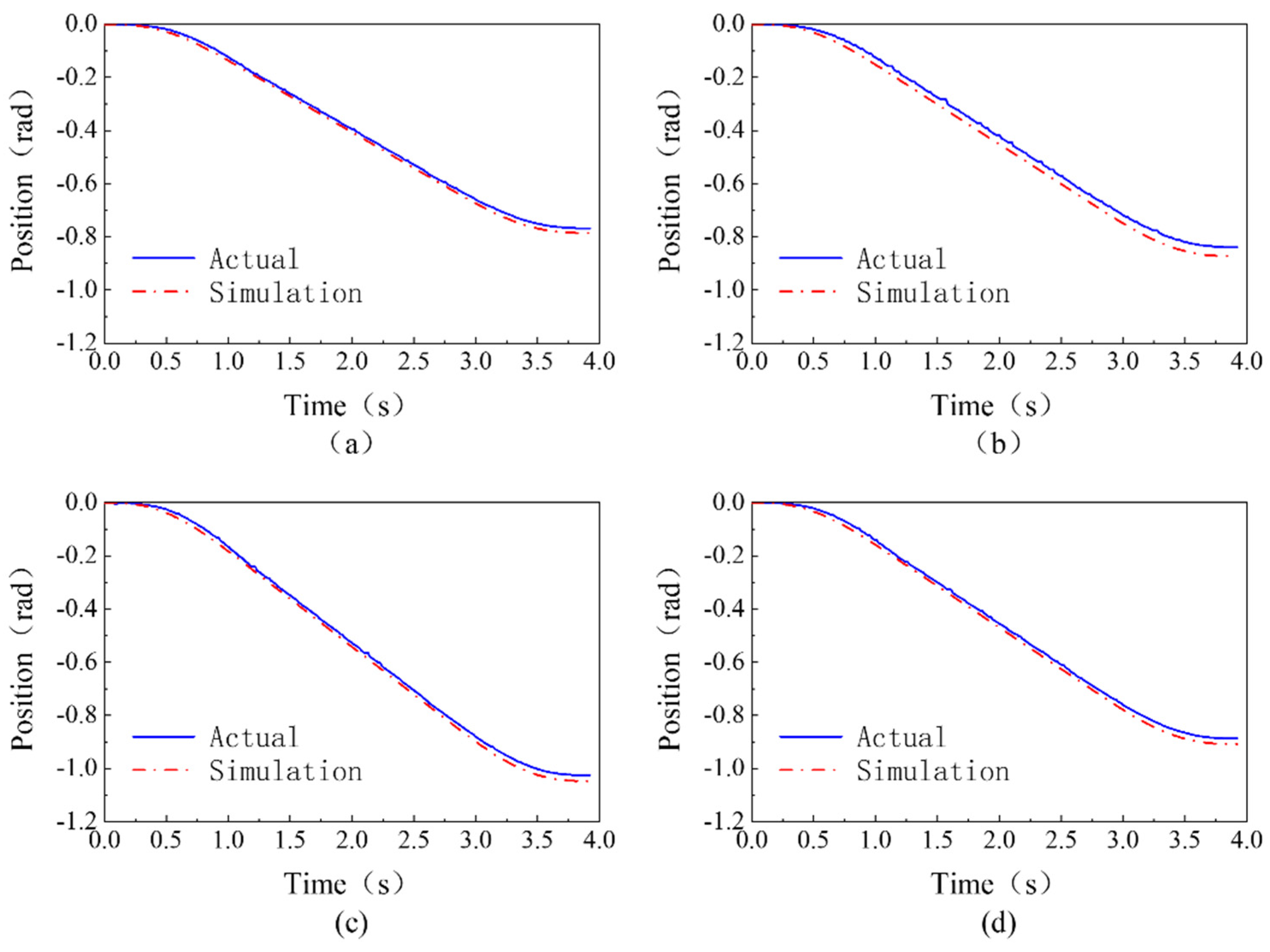
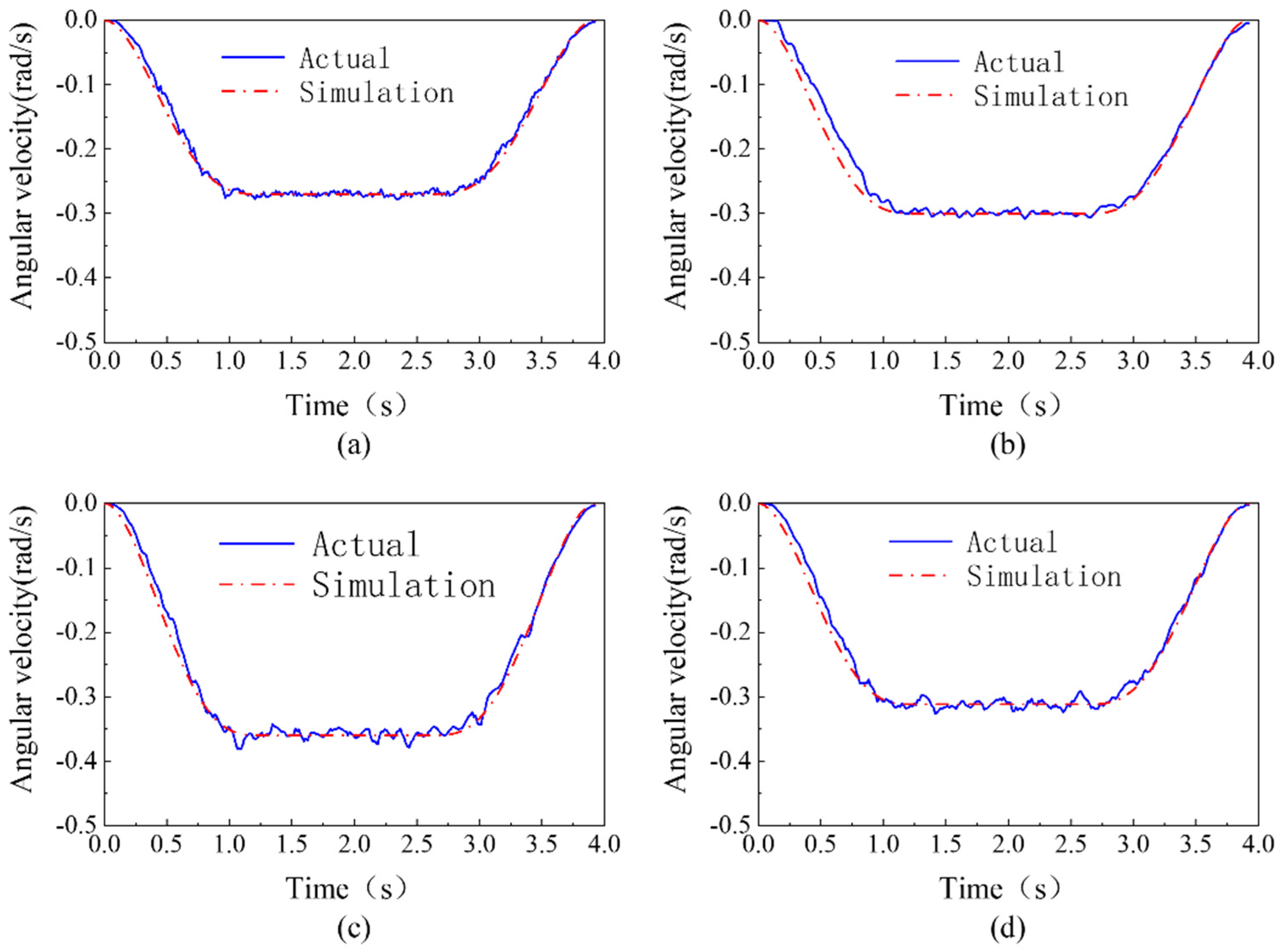
4.3. Multi-Joint Trajectory Planning Experiment

Trajectory planning for multiple joints was also performed. The initial position of each joint was assumed to be zero and the terminal position vectors were ${\theta }_f$ = (−0.7854, −0.8727, −1.0472, and −0.9075 rad). Constraints and parameters were the same as for Section 4.2, and the MWOA was applied to optimize the trajectory of each joint independently. As shown in

Table 4. Running time of each joint trajectory.

$\mathbf{Joint} \left(\mathit{i}\right)$	${\mathit{t}}_{\mathit{i}1}$	${\mathit{t}}_{\mathit{i}2}$	${\mathit{t}}_{\mathit{i}3}$
1	1.1957	1.2527	1.1167
2	1.1572	1.2805	1.2361
3	1.2345	1.3914	1.2948
4	1.2368	1.3308	1.2344

, the running times of each joint and each trajectory segment were all different. To ensure that constraints were satisfied as well as ensuring the synchronous motion of all joints, the maximum running time of each segment was selected to generate the trajectory; thus, the running time of each joint was $t$ = (1.2368, 1.3914, and 1.2948 s). The trajectories of each joint are shown in Figure 10. All trajectories were smooth, continuous, and satisfied constraints, similar to the single-joint experiments.

To verify the feasibility of the trajectory optimized by the MWOA, a simulation of the 4-DOF UEER robot moving along the planned trajectory was carried out. The end-effector trajectory of the 4-DOF UEER robot is shown in Figure 11. The simulation showed that the 4-DOF UEER robot moved steadily along the trajectory during the complete motion. Furthermore, the trajectory of the end-effector was smooth and continuous.

Finally, a pilot rehabilitation experiment was performed on a healthy volunteer. The volunteer was first familiarized with the content of the experiment and then made to wear the 4-DOF UEER robot and sit in a wheelchair with his arms relaxed. The 4-DOF UEER robot moved together with the volunteer’s arm along the planned trajectory, as depicted in Figure 12. Comparisons of position and angular velocity between the simulation and the actual are shown in Figure 13 and Figure 14. Among these joints, the maximum position errors were 0.033 rad (in joint 2), and the maximum angular velocity errors were 0.021 $\mathrm{r}\mathrm{a}\mathrm{d}/\mathrm{s}$ (in joint 3). The motion process remained stable and was completed safely, which verified the feasibility and practical value of the proposed MWOA.

5. Conclusions

In this paper, a multistrategy improved whale optimization algorithm (MWOA) was proposed for isokinetic rehabilitation trajectory planning with upper extremity exoskeleton rehabilitation robots. The main conclusions are as follows:

(1) A piecewise polynomial was used to construct the preliminary isokinetic rehabilitation trajectory. The trajectory included acceleration, uniform velocity, and deceleration, which meets the basic characteristics of isokinetic rehabilitation. Taking the minimum running time as the objective, the improved whale optimization algorithm was used to realize the bounded jerk trajectory in line with human motion. The simulation results have shown that the trajectory was continuous and smooth and without impact; moreover, the running time of the uniform velocity segment was the longest, indicating the feasibility of the trajectory;

(2) Compared with the original whale optimization algorithm, this proposed algorithm had a stronger global search ability, a higher convergence accuracy, a better robustness under complex constraints, and was more reliable and symmetrical in trajectory optimization. Compared with other excellent optimization algorithms, this algorithm also had a higher convergence accuracy and robustness;

(3) The upper extremity exoskeleton rehabilitation robot completed the simulated rehabilitation experiment safely and stably along the planned rehabilitation trajectory, indicating that the isokinetic rehabilitation trajectory planning of the upper extremity exoskeleton rehabilitation robot proposed in this paper was a feasible scheme.

As a result of the complexity of rehabilitation, further research is needed on rehabilitation trajectory planning, such as multi-objective trajectory planning.

References

1. Rodgers, H.; Bosomworth, H.; Krebs, H.I.; van Wijck, F.; Howel, D.; Wilson, N.; Aird, L.; Alvarado, N.; Andole, S.; Cohen, D.L.; et al. Robot assisted training for the upper limb after stroke (RATULS): A multicentre randomised controlled trial. Lancet 2019, 394, 51–62. [Google Scholar] [CrossRef] [PubMed] [Green Version]
2. Taveggia, G.; BorboNi, A.; SalVi, L.; MulÉ, C.; FoGliarEsi, S.; VillafaÑE, J.H.; CasalE, R. Efficacy of robot-assisted re-habilitation for the functional recovery of the upper limb in post-stroke patients: A randomized controlled study. Eur. J. Phys. Rehabil. Med. 2016, 52, 767–773. [Google Scholar] [PubMed]
3. Al-Quraishi, M.S.; Elamvazuthi, I.; Daud, S.A.; Parasuraman, S.; Borboni, A. EEG-Based Control for Upper and Lower Limb Exoskeletons and Prostheses: A Systematic Review. Sensors 2018, 18, 3342. [Google Scholar] [CrossRef] [PubMed] [Green Version]
4. Stinear, C.M.; Lang, C.E.; Zeiler, S.; Byblow, W.D. Advances and challenges in stroke rehabilitation. Lancet Neurol. 2020, 19, 348–360. [Google Scholar] [CrossRef]
5. Borboni, A.; Mor, M.; Faglia, R. Gloreha—Hand Robotic Rehabilitation: Design, Mechanical Model, and Experiments. J. Dyn. Syst. Meas. Control Trans. ASME 2016, 138, 111003. [Google Scholar] [CrossRef]
6. Tiboni, M.; Borboni, A.; Faglia, R.; Pellegrini, N. Robotics rehabilitation of the elbow based on surface electromyography signals. Adv. Mech. Eng. 2018, 10, 1687814018754590. [Google Scholar] [CrossRef]
7. Hong, C.; Rui, H.; Qiu, J.; Wang, Y.; Chaobin, Z.; Kecheng, S. A Survey of Rehabilitation Robot and Its Clinical Applications. Robot 2021, 43, 606–619. [Google Scholar]
8. Kim, B.; Ahn, K.-H.; Nam, S.; Hyun, D.J. Upper extremity exoskeleton system to generate customized therapy motions for stroke survivors. Robot. Auton. Syst. 2022, 154, 104128. [Google Scholar] [CrossRef]
9. Li, G.; Fang, Q.; Xu, T.; Zhao, J.; Cai, H.; Zhu, Y. Inverse kinematic analysis and trajectory planning of a modular upper limb rehabilitation exoskeleton. Technol. Health Care 2019, 27, 123–132. [Google Scholar] [CrossRef] [Green Version]
10. Yu, X.; Meng, W.; Liu, Z.; Ai, Q.; Liu, Q. Multi-objective Trajectory Optimization of Redundant Manipulator for Patient Assistance. In Proceedings of the 2021 27th International Conference on Mechatronics and Machine Vision in Practice (M2VIP), Shanghai, China, 26–28 November 2021; pp. 66–71. [Google Scholar] [CrossRef]
11. Wang, Z.; Li, Y.; Shuai, K.; Zhu, W.; Chen, B.; Chen, K. Multi-objective Trajectory Planning Method based on the Improved Elitist Non-dominated Sorting Genetic Algorithm. Chin. J. Mech. Eng. 2022, 35, 7. [Google Scholar] [CrossRef]
12. Parikh, P.A.; Trivedi, R.R.; Joshi, K.D. Trajectory planning of a 5 DOF feeding serial manipulator using 6th order polynomial method. J. Physics. Conf. Ser. 2021, 1921, 012088. [Google Scholar] [CrossRef]
13. Xu, J. Application of isokinetic exercise in rehabilitation evaluation and treatment. Chin. J. Phys. Med. Rehabil. 2006, 8, 570–573. [Google Scholar]
14. Kerimov, K.; Benlidayi, I.C.; Ozdemir, C.; Gunasti, O. The Effects of Upper Extremity Isokinetic Strengthening in Post-Stroke Hemiplegia: A Randomized Controlled Trial. J. Stroke Cerebrovasc. Dis. 2021, 30, 105729. [Google Scholar] [CrossRef] [PubMed]
15. Hammami, N.; Coroian, F.; Julia, M.; Amri, M.; Mottet, D.; Hérisson, C.; Laffont, I. Isokinetic muscle strengthening after acquired cerebral damage: A literature review. Ann. Phys. Rehabil. Med. 2012, 55, 279–291. [Google Scholar] [CrossRef] [PubMed] [Green Version]
16. Maharum, S.M.M.; Ishak, N.I.I.; Hussain, R.; Mansor, Z.; Rahim, S.Z.B.A.; Abdullah, M.M.A.B. Upper limb rehabilitation equipment with performance animation for isotonic and isokinetic exercises. AIP Conf. Proc. 2019, 2129, 020103. [Google Scholar]
17. Meng, X.; Zhu, X. Autonomous Obstacle Avoidance Path Planning for Grasping Manipulator Based on Elite Smoothing Ant Colony Algorithm. Symmetry 2022, 14, 1843. [Google Scholar] [CrossRef]
18. Patle, B.; Pandey, A.; Jagadeesh, A.; Parhi, D. Path planning in uncertain environment by using firefly algorithm. Def. Technol. 2018, 14, 691–701. [Google Scholar] [CrossRef]
19. Heidari, A.A.; Mirjalili, S.; Faris, H.; Aljarah, I.; Mafarja, M.; Chen, H. Harris hawks optimization: Algorithm and applications. Future Gener. Comput. Syst. 2019, 97, 849–872. [Google Scholar] [CrossRef]
20. Mirjalili, S.; Lewis, A. The Whale Optimization Algorithm. Adv. Eng. Softw. 2016, 95, 51–67. [Google Scholar] [CrossRef]
21. Zhao, J.; Zhu, X.; Meng, X.; Wu, X. Application of Improved Whale Optimization Algorithm in Time-optimal Trajectory Planning of Manipulator. Mech. Sci. Technol. Aerosp. Eng. 2021, 1–10. [Google Scholar] [CrossRef]
22. Gharehchopogh, F.S.; Gholizadeh, H. A comprehensive survey: Whale Optimization Algorithm and its applications. Swarm Evol. Comput. 2019, 48, 1–24. [Google Scholar] [CrossRef]
23. Li, M.; Xu, G.; Lai, Q.; Chen, J. A chaotic strategy-based quadratic Opposition-Based Learning adaptive variable-speed whale optimization algorithm. Math. Comput. Simul. 2021, 193, 71–99. [Google Scholar] [CrossRef]
24. Tong, W. A new whale optimisation algorithm based on self-adapting parameter adjustment and mix mutation strategy. Int. J. Comput. Integr. Manuf. 2020, 33, 949–961. [Google Scholar] [CrossRef]
25. Fan, Q.; Chen, Z.; Li, Z.; Xia, Z.; Yu, J.; Wang, D. A new improved whale optimization algorithm with joint search mecha-nisms for high-dimensional global optimization problems. Eng. Comput. 2021, 37, 1851–1878. [Google Scholar] [CrossRef]
26. Jiang, F.; Wang, L.; Bai, L. An Improved Whale Algorithm and Its Application in Truss Optimization. J. Bionic Eng. 2021, 18, 721–732. [Google Scholar] [CrossRef]
27. Elaziz, M.A.; Lu, S.; He, S. A multi-leader whale optimization algorithm for global optimization and image segmentation. Expert Syst. Appl. 2021, 175, 114841. [Google Scholar] [CrossRef]
28. Tizhoosh, H.R. Opposition-Based Learning: A New Scheme for Machine Intelligence. In Proceedings of the International Conference on Computational Intelligence for Modelling, Control and Automation and International Conference on Intelligent Agents, Web Technologies and Internet Commerce (CIMCA-IAWTIC’06), Vienna, Austria, 28–30 November 2005. [Google Scholar]
29. Rahnamayan, S.; Jesuthasan, J.; Bourennani, F.; Salehinejad, H.; Naterer, G.F. Computing opposition by involving entire population. In Proceedings of the 2014 IEEE Congress on Evolutionary Computation (CEC), Beijing, China, 6–11 July 2014. [Google Scholar]
30. Yuan, W.; You, X.; Liu, S. Dual-Population Ant Colony Algorithm on Dynamic Learning Mechanism. J. Front. Comput. Sci. Technol. 2019, 13, 1239–1250. [Google Scholar]
31. Kılıç, F.; Kaya, Y.; Yildirim, S. A novel multi population based particle swarm optimization for feature selection. Knowledge-Based Syst. 2021, 219, 106894. [Google Scholar] [CrossRef]
32. Du, Y.; Fan, Y.; Liu, P.; Tang, J.; Luo, Y. Multi-populations Covariance Learning Differential Evolution Algorithm. J. Electron. Inf. Technol. 2019, 41, 1488–1495. [Google Scholar]
33. Liu, X. Whale Optimization Algorithm for Multi-group with Information Exchange and Vertical and Horizontal Bidirectional Learning. J. Electron. Inf. Technol. 2021, 43, 3247–3256. [Google Scholar]
34. Chang, J.-J.; Tung, W.-L.; Wu, W.; Huang, M.-H.; Su, F.-C. Effects of Robot-Aided Bilateral Force-Induced Isokinetic Arm Training Combined with Conventional Rehabilitation on Arm Motor Function in Patients with Chronic Stroke. Arch. Phys. Med. Rehabil. 2007, 88, 1332–1338. [Google Scholar] [CrossRef]
35. Nguiadem, C.; Raison, M.; Achiche, S. Motion Planning of Upper-Limb Exoskeleton Robots: A Review. Appl. Sci. 2020, 10, 7626. [Google Scholar] [CrossRef]
36. Frisoli, A.; Loconsole, C.; Bartalucci, R.; Bergamasco, M. A new bounded jerk on-line trajectory planning for mimicking human movements in robot-aided neurorehabilitation. Robot. Auton. Syst. 2013, 61, 404–415. [Google Scholar] [CrossRef]
37. Qie, X.; Kang, C.; Zong, G.; Chen, S. Trajectory Planning and Simulation Study of Redundant Robotic Arm for Upper Limb Rehabilitation Based on Back Propagation Neural Network and Genetic Algorithm. Sensors 2022, 22, 4071. [Google Scholar] [CrossRef] [PubMed]
38. Yuan, Y.; Dang, Q.; Xu, W.; Liu, L.; Luo, Y. Dynamic Penalty Function Method for Constrained Optimization Problem. Comput. Eng. Appl. 2022, 58, 83. [Google Scholar]
39. Gharehchopogh, F.S. An Improved Tunicate Swarm Algorithm with Best-random Mutation Strategy for Global Optimization Problems. J. Bionic Eng. 2022, 19, 1177–1202. [Google Scholar] [CrossRef]
40. Zhao, S.; Wang, P.; Heidari, A.A.; Zhao, X.; Ma, C.; Chen, H. An enhanced Cauchy mutation grasshopper optimization with trigonometric substitution: Engineering design and feature selection. Eng. Comput. 2021, 38, 4583–4616. [Google Scholar] [CrossRef]
41. Xu, L.; Cao, M.; Song, B. A new approach to smooth path planning of mobile robot based on quartic Bezier transition curve and improved PSO algorithm. Neurocomputing 2022, 473, 98–106. [Google Scholar] [CrossRef]
42. Yang, X. Firefly Algorithm, Stochastic Test Functions and Design Optimisation. Int. J. Bio-Inspired Comput. 2010, 2, 78–84. [Google Scholar] [CrossRef]
43. Mirjalili, S.; Gandomi, A.H.; Mirjalili, S.Z.; Saremi, S.; Faris, H.; Mirjalili, S.M. Salp Swarm Algorithm: A bio-inspired optimizer for engineering design problems. Adv. Eng. Softw. 2017, 114, 163–191. [Google Scholar] [CrossRef]
Figure 1. Diagram of the proposed communication mechanism between dual subpopulations. Note that the comparator performs the operation of Equations (13) and (14).
Symmetry 15 00232 g001
Figure 2. Population distributions obtained by the WOA, COBLWOA, and LCOBLWOA. (ac) The population distribution obtained by the WOA at the 1st, 60th, and 84th iteration, respectively. (df) The population distribution obtained by the COBLWOA at the 1st, 60th, and 84th iteration, respectively. (gi) The population distribution obtained by the LCOBLWOA at the 1st, 60th, and 84th iteration, respectively.
Symmetry 15 00232 g002
Figure 3. Convergence curves obtained with the WOA, COBLWOA, and LCOBLWOA.
Symmetry 15 00232 g003
Figure 4. Mutation trend for the LCOBLWOA.
Symmetry 15 00232 g004
Figure 5. The 4-DOF UEER robot.
Symmetry 15 00232 g005
Figure 6. Running time trend of the MWOA and the WOA.
Symmetry 15 00232 g006
Figure 7. Comparison of the trajectories optimized by the MWOA and the WOA. (a) A comparison of the position curves optimized by the MWOA and the WOA. (b) A comparison of the angular velocity curves optimized by the MWOA and the WOA. (c) A comparison of the angular acceleration curves optimized by the MWOA and the WOA. (d) A comparison of the jerk curves optimized by the MWOA and the WOA.
Symmetry 15 00232 g007
Figure 8. Convergence curves of the MWOA and the WOA. (a) Fitness convergence curves of the MWOA and the WOA. (b) Running time convergence curves of the MWOA. (c) Running time convergence curves of the WOA.
Symmetry 15 00232 g008
Figure 9. Fitness convergence curves of the PSO, FA, SSA, WOA, IWOA, and MWOA.
Symmetry 15 00232 g009
Figure 10. Trajectories of each joint. (a) Position curves of each joint. (b) Angular velocity curves of each joint. (c) Angular acceleration curves of each joint. (d) Jerk curves of each joint.
Symmetry 15 00232 g010
Figure 11. The end-effector trajectory.
Symmetry 15 00232 g011
Figure 12. Pilot experiment on a healthy volunteer.
Symmetry 15 00232 g012
Figure 13. Comparisons of position between the simulation and the actual. (ad) represent the comparisons of position between the simulation and the actual of joints 1 to 4, respectively.
Symmetry 15 00232 g013
Figure 14. Comparisons of angular velocity between the simulation and the actual. (ad) represent the comparisons of angular velocity between the simulation and the actual of joints 1 to 4, respectively.
Symmetry 15 00232 g014