A Family of Higher Order Scheme for Multiple Roots

Abstract

We have developed a two-point iterative scheme for multiple roots that achieves fifth order convergence by using two function evaluations and two derivative evaluations each iteration. Weight function approach is utilized to frame the scheme. The weight function named as $R\left({\upsilon }_t\right)$ is used, which is a function of ${\upsilon }_t$, and ${\upsilon }_t$ is a function of ${\omega }_t$, i.e., ${\upsilon }_t=\frac{{\omega }_t}{1+a{\omega }_t},$ where a is a real number and ${\omega }_t={\left(\frac{g\left({\mathtt{y}}_t\right)}{g\left({\mathtt{x}}_t\right)}\right)}^{\frac{1}{\tilde{m}}}$ is a multi-valued function. The consistency of the newly generated methods is ensured numerically and through the basins of attraction. Four complex functions are considered to compare the new methods with existing schemes via basins of attraction, and all provided basins of attraction possess reflection symmetry. Further, five numerical examples are used to verify the theoretical results and to contrast the presented schemes with some recognized schemes of fifth order. The results obtained have proved that the new schemes are better than the existing schemes of the same nature.

1. Introduction

The approximate solution of a function $g,$ where $g:\mathbb{C}\to \mathbb{C}$, is a complex valued function possessing the nth order derivatives and roots with multiplicity $\tilde{m}>1,$ can be evaluated through iterative methods. These types of methods have attracted interest for some recent research [1,2], including symmetry-related works [3,4,5,6]. There are two types of iterative methods which can serve the purpose: one-point iterative methods and multi-point iterative methods. One-point iterative methods of order $\rho$ use high order derivatives, namely $g^{\left(1\right)}\left(\mathtt{x}\right),g^{\left(2\right)}\left(\mathtt{x}\right),\dots ,g^{(\rho -1)}\left(\mathtt{x}\right)$ of function $g.$ For example, the methods presented by Chun et al. [7], Hansen et al. [8], Neta [9], Osada [10] and Sharma et al. [11] are some one-point iterative methods. However, it is very difficult to find out the higher order derivatives when the function g is complex. To reduce this ambiguity, multi-point iterative methods are used as they are free to use any number of evaluations of derivatives. In most of the multi-point iterative methods, the most reputable modified Newton–Raphson’s Method [12] for multiple roots of a non linear function is used as the first step, sometimes as it is and sometimes by making some modifications to it. The scheme for modified Newton–Raphson’s Method is

$${\mathtt{x}}_{t+1}={\mathtt{x}}_t-\tilde{m}\frac{g\left({\mathtt{x}}_t\right)}{g^{\prime }\left({\mathtt{x}}_t\right)},t=0,1,2,\dots$$

(1)

This method has quadratic order of convergence for $\tilde{m}\ge 1$. The multipoint iterative methods by Zhou et al. [13], Geum et al. [14,15] and Behl et al. [16] have used a modified Newton’s method as the first phase of their suggested schemes. Further, the methods by Li et al. [17], Zhou et al. [18], Behl et al. [19], Kansal et al. [20] and Rani et al. [21] are some examples of multi-point iterative methods whose first step is based upon a modified Newton–Raphson’s method.

From the literature, one can observe that the primary goal behind the construction of the multi-point iterative method is to bring the order of convergence as high as possible without using the higher order derivatives. Different types of approaches [22,23,24,25,26,27,28,29] (for example, quadrature formula, adomian polynomial, divided difference approach, the weight function approach) have been applied by researchers to develop the multi-point iterative methods. Below, we provide some of the multi-point methods which are based on a weight function approach. In 2015, Artidiello et al. [30] developed a two-point scheme using weight function as follows:

$$\begin{array}{cc}\hfill {\mathtt{y}}_t& ={\mathtt{x}}_t-\beta \frac{g\left({\mathtt{x}}_t\right)}{g^{\prime }\left({\mathtt{x}}_t\right)},\hfill \\ \hfill {\mathtt{x}}_{t+1}& ={\mathtt{y}}_t-H\left({\mu }_t\right)\frac{g\left({\mathtt{y}}_t\right)}{g^{\prime }\left({\mathtt{x}}_t\right)},\hfill \end{array}$$

(2)

where $H:\mathbb{R}\to \mathbb{R}$ is weight function, ${\mu }_t=\frac{a_{1}g\left({\mathtt{x}}_t\right)+a_{2}g\left({\mathtt{y}}_t\right)}{b_{1}g\left({\mathtt{x}}_t\right)+b_{2}g\left({\mathtt{y}}_t\right)}$, and $\beta ,a_1,a_2,b_1$ and $b_2$ are real parameters.

Very recently, in August 2022, Cordero et al. [31] developed a new iterative scheme with the help of weight function, which is given below:

$$\begin{array}{cc}\hfill {\mathtt{y}}_t& ={\mathtt{x}}_t-\beta \frac{g\left({\mathtt{x}}_t\right)}{g^{\prime }\left({\mathtt{x}}_t\right)},\hfill \\ \hfill {\mathtt{x}}_{t+1}& ={\mathtt{y}}_t-H\left(u_t\right)\frac{g\left({\mathtt{x}}_t\right)}{g^{\prime }\left({\mathtt{y}}_t\right)},\hfill \end{array}$$

(3)

where $H:\mathbb{R}\to \mathbb{R}$ is weight function, $u_t=\frac{g^{\prime }\left({\mathtt{y}}_t\right)}{g^{\prime }\left({\mathtt{x}}_t\right)}$ and $\beta$ is a free parameter.

Further, Chanu et al. [32] created a new scheme using the weight function and divided difference in September 2022, as follows:

$$\begin{array}{cc}\hfill {\mathtt{y}}_t& ={\mathtt{x}}_t-\frac{g\left({\mathtt{x}}_t\right)}{g^{\prime }\left({\mathtt{x}}_t\right)},\hfill \\ \hfill {\mathtt{x}}_{t+1}& ={\mathtt{y}}_t-H\left(v_t\right)\frac{g\left({\mathtt{y}}_t\right)(1+\frac{A}{2})}{g[{\mathtt{y}}_t,{\mathtt{x}}_t]},\hfill \end{array}$$

(4)

where $A=\frac{g\left({\mathtt{y}}_t\right)(g^{\prime }\left({\mathtt{x}}_t\right)-g[{\mathtt{y}}_t,{\mathtt{x}}_t])}{g\left({\mathtt{x}}_t\right)g[{\mathtt{y}}_t,{\mathtt{x}}_t]},$ $H:\mathbb{R}\to \mathbb{R}$ is weight function, and $v_t=\frac{g\left({\mathtt{y}}_t\right)}{g\left({\mathtt{x}}_t\right)}$.

Motivated by this weight function approach, we are fully concentrated on developing a multi-point iterative method for multiple roots of order five which uses two function evaluations and two derivative evaluations per iteration. The first step of our new scheme is also a modified Newton–Raphson’s Method, and the second step involves a weight function. Mathematica [33] is used in the whole work for symbolic and numerical computation.

The outline of the rest of the paper is as follows: Section 2 of the paper includes the development of the new family and also an investigation of its convergence. Section 3 discusses a few distinctive members of the newly formed family. The basins of attraction are contained in Section 4 of the paper. The theoretical findings are validated in Section 5 by a number of numerical instances. Finally, Section 6 includes the closing remarks.

2. Construction of the Fifth-Order Family

Here, we derive a fifth-order mechanism for multiple zeros $(\tilde{m}\ge 2)$ in the following, by considering the scheme:

$$\begin{array}{cc}\hfill {\mathtt{y}}_t& ={\mathtt{x}}_t-\tilde{m}\frac{g\left({\mathtt{x}}_t\right)}{g^{\prime }\left({\mathtt{x}}_t\right)},\hfill \\ \hfill {\mathtt{x}}_{t+1}& ={\mathtt{y}}_t-\tilde{m}R\left({\upsilon }_t\right)\frac{g\left({\mathtt{y}}_t\right)}{g^{\prime }\left({\mathtt{y}}_t\right)},\hfill \end{array}$$

(5)

where $\tilde{m}\ge 2$ is the multiplicity of the required zero and $R\left({\upsilon }_t\right)$ is a single variable weight function. Moreover, ${\upsilon }_t=\frac{{\omega }_t}{1+a{\omega }_t},$ where $a\in \mathbb{R}$ and ${\omega }_t={\left(\frac{g\left({\mathtt{y}}_t\right)}{g\left({\mathtt{x}}_t\right)}\right)}^{\frac{1}{\tilde{m}}}$ are multi-valued functions.

Theorem 1.

Let $\alpha \in D$ be a multiple root with multiplicity $\tilde{m}\ge 2$ of a holomorphic function $g:D\subset \mathbb{C}\to \mathbb{C}$ for an open interval $D.$ If $x_0$ is sufficiently close to α then the new Scheme (5) has fifth-order of convergence, provided

$$R\left(0\right)=1,R^{\prime }\left(0\right)=0,R^{″}\left(0\right)=2,\left|R^{‴}\left(0\right)\right|<\infty ,$$

(6)

and fulfils the aforementioned error equation,

$$e_{t+1}=\left(\frac{(18+12a+6\tilde{m}-R^{‴}\left(0\right))D_1^4-12\tilde{m}{D}_1^2{D}_2}{6{\tilde{m}}^4}\right)e_t^5+O\left(e_t^6\right).$$

(7)

Proof of Theorem 1.

If ${\mathtt{x}}_t$ and $e_t$ denote the approximate solution and the corresponding error in t–th iteration, then $e_t={\mathtt{x}}_t-\alpha .$

For the function $g\left({\mathtt{x}}_t\right),$ apply Taylor’s series expansion about $\mathtt{x}=\alpha ,$

$$g\left({\mathtt{x}}_t\right)=g\left(\alpha \right)+g^{\left(1\right)}\left(\alpha \right)e_t+\frac{g^{\left(2\right)}\left(\alpha \right)}{2!}{e}_t^2+...+\frac{g^{(\tilde{m}-1)}\left(\alpha \right)}{\tilde{m}-1!}{e}_t^{\tilde{m}-1}+\frac{g^{\left(\tilde{m}\right)}\left(\alpha \right)}{\tilde{m}!}{e}_t^{\tilde{m}}+\dots$$

(8)

since the root $\alpha$ has multiplicity $\tilde{m}$. Therefore, $g\left(\alpha \right)=g^{\left(1\right)}\left(\alpha \right)=g^{\left(2\right)}\left(\alpha \right)=\dots g^{(\tilde{m}-1)}\left(\alpha \right)=0$ and $g^{\left(\tilde{m}\right)}\left(\alpha \right)\ne 0.$ Thus, Equation (8) becomes

$$g\left({\mathtt{x}}_t\right)=\frac{g^{\left(\tilde{m}\right)}\left(\alpha \right)}{\tilde{m}!}{e}_t^{\tilde{m}}\left(1+D_1{e}_t+D_2{e}_t^2+D_3{e}_t^3+D_4{e}_t^4+D_5{e}_t^5+O\left(e_t^6\right)\right).$$

(9)

Here, the asymptotic error constants $D_i=\frac{\tilde{m}!}{(\tilde{m}+i)!}\frac{g^{(\tilde{m}+i)}\left(\alpha \right)}{g^{\left(\tilde{m}\right)}\left(\alpha \right)},i=1,2,3,\dots$

$$\begin{array}{c}\hfill g^{\prime }\left({\mathtt{x}}_t\right)=\frac{g^{\left(\tilde{m}\right)}\left(\alpha \right)}{(\tilde{m}-1)!}{e}_t^{\tilde{m}-1}[1+\left(\frac{1+\tilde{m}}{\tilde{m}}\right)D_1{e}_t+\left(\frac{2+\tilde{m}}{\tilde{m}}\right)D_2{e}_t^2+\left(\frac{3+\tilde{m}}{\tilde{m}}\right)D_3{e}_t^3\\ \hfill \left(\frac{4+\tilde{m}}{\tilde{m}}\right)D_4{e}_t^4+\left(\frac{5+\tilde{m}}{\tilde{m}}\right)D_5{e}_t^5+O\left(e_t^6\right)].\end{array}$$

(10)

Dividing (9) by (10), we obtain

$$\begin{array}{c}\hfill \frac{g\left({\mathtt{x}}_t\right)}{g^{\prime }\left({\mathtt{x}}_t\right)}=\frac{e_t}{\tilde{m}}-\frac{D_1}{{\tilde{m}}^2}{e}_t^2+\frac{[(1+\tilde{m})D_1^2-2\tilde{m}{D}_2]}{{\tilde{m}}^3}{e}_t^3+\frac{L^{\prime }}{{\tilde{m}}^4}{e}_t^4+\frac{L}{{\tilde{m}}^5}{e}_t^5+O\left(e_t^6\right),\end{array}$$

(11)

where $L^{\prime }=[-{(1+\tilde{m})}^2{D}_1^3+\tilde{m}(4+3\tilde{m})D_1{D}_2-3{\tilde{m}}^2{D}_3],$ $L=({(1+\tilde{m})}^3{D}_1^4-2\tilde{m}(3+5\tilde{m}+2{\tilde{m}}^2)D_1^2{D}_2+2{\tilde{m}}^2(3+2\tilde{m})D_1{D}_3$ $+2{\tilde{m}}^2[(2+\tilde{m})D_2^2-2\tilde{m}{D}_4]).$

Put (11) in the first step of (5),

$$\begin{array}{c}\hfill e_{{\mathtt{y}}_t}=\frac{D_1}{\tilde{m}}{e}_t^2+\left(\frac{2\tilde{m}{D}_2-(1+\tilde{m})D_1^2}{{\tilde{m}}^2}\right)e_t^3+\left(\frac{-L^{\prime }}{{\tilde{m}}^3}\right)e_t^4+O\left(e_t^5\right).\end{array}$$

(12)

Now, we have

$$\begin{array}{c}\hfill g\left({\mathtt{y}}_t\right)=\frac{g^{\left(\tilde{m}\right)}\left(x_0\right)}{\tilde{m}!}{e}_{{\mathtt{y}}_k}^{\tilde{m}}\left(1+D_1{e}_{{\mathtt{y}}_k}+D_2{e}_{{\mathtt{y}}_k}^2+D_3{e}_{{\mathtt{y}}_k}^3+D_4{e}_{{\mathtt{y}}_k}^4+D_5{e}_{{\mathtt{y}}_k}^5+O\left(e_{{\mathtt{y}}_k}^6\right)\right),\end{array}$$

(13)

and

$$\begin{array}{cc}\hfill g^{\prime }\left({\mathtt{y}}_t\right)=& \frac{g^{\left(\tilde{m}\right)}\left(\alpha \right)}{(\tilde{m}-1)!}{e}_{{\mathtt{y}}_k}^{\tilde{m}-1}[1+\left(\frac{1+\tilde{m}}{\tilde{m}}\right)D_1{e}_{{\mathtt{y}}_k}+\left(\frac{2+\tilde{m}}{\tilde{m}}\right)D_2{e}_{{\mathtt{y}}_k}^2+\left(\frac{3+\tilde{m}}{\tilde{m}}\right)D_3{e}_{{\mathtt{y}}_k}^3\hfill \\ \hfill & +\left(\frac{4+\tilde{m}}{\tilde{m}}\right)D_4{e}_{{\mathtt{y}}_k}^4+\left(\frac{5+\tilde{m}}{\tilde{m}}\right)D_5{e}_{{\mathtt{y}}_k}^5+O\left(e_{{\mathtt{y}}_k}^6\right)].\hfill \end{array}$$

(14)

Divide (13) by (9),

$$\begin{array}{cc}\hfill \frac{g\left({\mathtt{y}}_t\right)}{g\left(x_t\right)}=& \left(\frac{D_1}{\tilde{m}}\right)e^{\tilde{m}}\left(1+\frac{L_1}{D_1}{e}_t+\frac{L_2}{2\tilde{m}{D}_1^2}{e}_t^2+\frac{L_3}{6{\tilde{m}}^2{D}_1^3}{e}_t^3+o\left(e_t^4\right)\right),\hfill \end{array}$$

(15)

where $L_1=2\tilde{m}{D}_2-(2+\tilde{m})D_1^2,$ $L_2={(1+\tilde{m})}^2(3+\tilde{m})D_1^4-2\tilde{m}(3+5\tilde{m}+2{\tilde{m}}^2)D_1^2{D}_2+4{\tilde{m}}^2(\tilde{m}-1)D_2^2+6{\tilde{m}}^2{D}_1{D}_3,$ $L_3=-{(\tilde{m}+1)}^3({\tilde{m}}^2+6\tilde{m}+8)D_1^6+6\tilde{m}({\tilde{m}}^4+6{\tilde{m}}^3+13{\tilde{m}}^2+13\tilde{m}+4)D_1^4{D}_2+8{\tilde{m}}^3({\tilde{m}}^2-3\tilde{m}+2)D_2^3+6{\tilde{m}}^2{D}_1^3(3{\tilde{m}}^2+7\tilde{m}+4)D_3+36{\tilde{m}}^3(\tilde{m}-1)D_1{D}_2{D}_3-12{\tilde{m}}^3{D}_1^2[{(\tilde{m}+1)}^2{D}_2^2-2D_4].$

Also,

$$\begin{array}{cc}\hfill {\omega }_t={\left(\frac{g\left({\mathtt{y}}_t\right)}{g\left(x_t\right)}\right)}^{1/\tilde{m}}=& \frac{D_1}{\tilde{m}}{e}^{\tilde{m}}+\frac{L_1}{{\tilde{m}}^2}{e}_t^2+\frac{M_1}{2{\tilde{m}}^3}{e}_t^3+\frac{M_2}{6{\tilde{m}}^4}{e}_t^4+o\left(e_t^5\right),\hfill \end{array}$$

(16)

where $M_1=[(7+\tilde{m}(7+2\tilde{m}))D_1^3-2\tilde{m}(7+3\tilde{m})D_1{D}_2+6{\tilde{m}}^2{D}_3],$ $M_2=[-(2+\tilde{m})(17+\tilde{m}(17+6\mathsf{m}))D_1^4+6\tilde{m}(17+4\tilde{m}(4+\tilde{m}))D_1^2{D}_2-12{\tilde{m}}^2(5+2\tilde{m})D_1{D}_3+12{\tilde{m}}^2(-(3+\tilde{m})D_2^2+2\tilde{m}{D}_4)].$

From Scheme (5), we have ${\upsilon }_t=\frac{{\omega }_t}{1+a{\omega }_t}$. Using (16) in it, we obtain

$$\begin{array}{c}\hfill {\upsilon }_t=\frac{D_1}{\tilde{m}}{e}_t^{\tilde{m}}+\frac{2\tilde{m}{D}_2-(2+a+\tilde{m})D_1^2}{{\tilde{m}}^2}{e}_t^2+\frac{N_1}{2{\tilde{m}}^3}{e}_t^3+\frac{N_2}{6{\tilde{m}}^4}{e}_t^4+o\left(e_t^5\right),\end{array}$$

(17)

where $N_1=[(7+2a^2+\tilde{m}(7+2\tilde{m})+4a(2+\tilde{m}))D_1^3-2\tilde{m}(7+4a+3\tilde{m})D_1{D}_2+6{\tilde{m}}^2{D}_3],$ $N_2=[(34+6a^3+51\tilde{m}+29{\tilde{m}}^2+6{\tilde{m}}^3+18a^2(2+\tilde{m})+6a(11+11\tilde{m}+3{\tilde{m}}^2))D_1^4-6\tilde{m}(17+6a^2+16\tilde{m}+4{\tilde{m}}^2+2a(11+5\tilde{m}))D_1^2{D}_2+12{\tilde{m}}^2(5+3a+2\tilde{m})D_1{D}_3+12{\tilde{m}}^2((3+2a+\tilde{m})D_2^2-2\tilde{m}{D}_4)].$

Expanding weight function $R\left({\upsilon }_t\right)$ around the locality of origin, as follows,

$$R\left({\upsilon }_t\right)=R\left(0\right)+R^{\prime }\left(0\right){\upsilon }_t+\frac{1}{2!}{R}^{″}\left(0\right){\upsilon }_t^2+\frac{1}{3!}{R}^{‴}\left(0\right){\upsilon }_t^3+\dots$$

(18)

At last, using the result of step one of schemes (5), (13), ( 14) and (18) in the second step of Mechanism (5), we obtain

$$\begin{array}{cc}\hfill e_{t+1}& =-\frac{[-1+R\left(0\right)]D_1}{\tilde{m}}{e}_t^2+\frac{[-2(-1+R\left(0\right))\tilde{m}{D}_2+D_1^2((-1+R\left(0\right))(1+\tilde{m})-R^{\prime }\left(0\right)]}{{\tilde{m}}^2}{e}_t^3\hfill \\ & +\frac{Q_1}{2{\tilde{m}}^3}{e}_t^4+\frac{Q_2}{6{\tilde{m}}^4}{e}_t^5+O\left(e_t^6\right),\hfill \end{array}$$

(19)

where $Q_1=(-6(-1+R\left(0\right)){\tilde{m}}^2{D}_3+2\tilde{m}{D}_1{D}_2((-1+R\left(0\right))(4+3\tilde{m})-4R^{\prime }\left(0\right))+D_1^3(2+4\tilde{m}-4\tilde{m}(R\left(0\right)+2{\tilde{m}}^2-2R\left(0\right){\tilde{m}}^2+2(3+a+2\tilde{m})R^{\prime }\left(0\right)-R^{″}\left(0\right))),$ $Q_2=(12{\tilde{m}}^2(-2(-1+R\left(0\right))\tilde{m}{D}_4+D_2^2((-1+R\left(0\right))(2+\tilde{m})-2R^{\prime }\left(0\right)))+12{\tilde{m}}^2{D}_1{D}_3((-1+R\left(0\right))(3+2\tilde{m})-3R^{\prime }\left(0\right))+6\tilde{m}{D}_1^2{D}_2(2(-3+R\left(0\right)-5\tilde{m}+5R\left(0\right)\tilde{m}-2{\tilde{m}}^2+2R\left(0\right){\tilde{m}}^2)-(17+6a+10\tilde{m})R^{\prime }\left(0\right)+3R^{″}\left(0\right))+D_1^4(-6-6R\left(0\right)-18\tilde{m}+6R\left(0\right)\tilde{m}-18{\tilde{m}}^2+18R\left(0\right){\tilde{m}}^2-6{\tilde{m}}^3+6R\left(0\right){\tilde{m}}^3-3(11+2a^2+17\tilde{m}+6{\tilde{m}}^2+2a(5+3\tilde{m}))R^{\prime }\left(0\right)+3(5+2a+3\tilde{m})R^{″}\left(0\right)-R^{‴}\left(0\right)).$

Using the Expression (19), we can quickly determine that Mechanism (5) obtains the convergence of at least fifth-order, if

$$R\left(0\right)=1,R^{\prime }\left(0\right)=0,R^{″}\left(0\right)=2.$$

(20)

Next, by using (20) in (19), we obtain

$$e_{t+1}=\left(\frac{(18+12a+6\tilde{m}-R^{‴}\left(0\right))D_1^4-12\tilde{m}{D}_1^2{D}_2}{6{\tilde{m}}^4}\right)e_t^5+O\left(e_t^6\right),$$

(21)

Provided $\left|R^{‴}\left(0\right)\right|<\infty .$ Hence, Scheme (5) has fifth-order convergence.    □

3. Special Cases

This section provides the new methods of fifth order for multiple roots by making different choices of weight functions adhering the constraints of Theorem 1. A few special cases are stated in the preceding

Table 1. Some special cases of Mechanism (5).

Cases (Naming)	Weight Functions	Equivalent Iterative Method
Case-1 (TM1)	$R\left({\upsilon }_t\right)=1+{\upsilon }_t^2$	${\mathtt{y}}_t={\mathtt{x}}_t-\tilde{m}\frac{g\left({\mathtt{x}}_t\right)}{g^{\prime }\left({\mathtt{x}}_t\right)},$
		${\mathtt{x}}_{t+1}={\mathtt{y}}_t-\tilde{m}(1+{\upsilon }_t^2)\frac{g\left({\mathtt{y}}_t\right)}{g^{\prime }\left({\mathtt{y}}_t\right)}$.
Case-2 (TM2)	$R\left({\upsilon }_t\right)=e^{-{\upsilon }_t}+{\upsilon }_t+\frac{{\upsilon }_t^2}{2}$	${\mathtt{y}}_t={\mathtt{x}}_t-\tilde{m}\frac{g\left({\mathtt{x}}_t\right)}{g^{\prime }\left({\mathtt{x}}_t\right)},$
		${\mathtt{x}}_{t+1}={\mathtt{y}}_t-\tilde{m}(e^{-{\upsilon }_t}+{\upsilon }_t+\frac{{\upsilon }_t^2}{2})\frac{g\left({\mathtt{y}}_t\right)}{g^{\prime }\left({\mathtt{y}}_t\right)}$.
Case-3 (TM3)	$R\left({\upsilon }_t\right)=(1-{\upsilon }_t)e^{{\upsilon }_t}+\frac{3}{2}{\upsilon }_t^2$	${\mathtt{y}}_t={\mathtt{x}}_t-\tilde{m}\frac{g\left({\mathtt{x}}_t\right)}{g^{\prime }\left({\mathtt{x}}_t\right)},$
		${\mathtt{x}}_{t+1}={\mathtt{y}}_t-\tilde{m}((1-{\upsilon }_t)e^{{\upsilon }_t}+\frac{3}{2}{\upsilon }_t^2)\frac{g\left({\mathtt{y}}_t\right)}{g^{\prime }\left({\mathtt{y}}_t\right)}$.
Case-4 (TM4)	$R\left({\upsilon }_t\right)=2-{\upsilon }_t-\frac{1}{1+{\upsilon }_t}+2{\upsilon }_t^2$	${\mathtt{y}}_t={\mathtt{x}}_t-\tilde{m}\frac{g\left({\mathtt{x}}_t\right)}{g^{\prime }\left({\mathtt{x}}_t\right)},$
		${\mathtt{x}}_{t+1}={\mathtt{y}}_t-\tilde{m}(2-{\upsilon }_t-\frac{1}{1+{\upsilon }_t}+2{\upsilon }_t^2)\frac{g\left({\mathtt{y}}_t\right)}{g^{\prime }\left({\mathtt{y}}_t\right)}$.

.

4. Basins of Attraction

The graphical images known as the basins of attraction of the roots of a polynomial $g\left(w\right)$ in the Complex plane are used to inspect the convergence of the scheme. The major significance of using the basins of attraction is that it widens the scope of inceptive guesses to obtain the zeros of an equation. These graphical images have been used by many researchers [34,35,36,37,38,39,40,41,42] to measure the stability and effectiveness of the iterative formulae. We use ${10}^{-3}$ as tolerance, with a maximum of 25 iterations to exhibit the basins. The procedure is closed down with the comment that the iteration method starting from $w_0$ is divergent, if the tolerance is not gained in the needed number of iterations. There are some basic rules that are used to draw the basins of attraction, given as below:

• The first rule is to select a rectangular area and make sure that every root of the considered polynomial lies inside this region.
• Each initial guess of a root is given a color in the basins of attraction. Similarly, another color is given to each initial guess of another root in the basins of attraction. For each of the complex polynomial’s roots, this operation is repeated.
• If the iterative formula which started with the initial approximation $w_0$ converges to a root, then the basins of attraction display the color which is allotted to the initial guess of that root at point $w_0.$ Otherwise, the initial guess $w_0$ is painted with black color.

We now proceed to compare our newly proposed methods, TM1, TM2, TM3 and TM4, with some existing schemes of the same nature. For comparison, we consider the three subcases of the scheme by Sharma et al. [40] and three subcases of the family presented by Chanu et al. [41]. The first method developed by Sharma et al. [40], which we denoted by SM1, is given as:

$$\begin{array}{cc}\hfill {\mathtt{y}}_t& ={\mathtt{x}}_t-\tilde{m}\frac{g\left({\mathtt{x}}_t\right)}{g^{\prime }\left({\mathtt{x}}_t\right)},\hfill \\ \hfill {\mathtt{x}}_{t+1}& ={\mathtt{y}}_t-\tilde{m}(1+{\omega }_t^2)\frac{g\left({\mathtt{y}}_t\right)}{g^{\prime }\left({\mathtt{y}}_t\right)}.\hfill \end{array}$$

(22)

We designate the second subcase of the method by Sharma et al. [40] as SM2, which is given below:

$$\begin{array}{cc}\hfill {\mathtt{y}}_t& ={\mathtt{x}}_t-\tilde{m}\frac{g\left({\mathtt{x}}_t\right)}{g^{\prime }\left({\mathtt{x}}_t\right)},\hfill \\ \hfill {\mathtt{x}}_{t+1}& ={\mathtt{y}}_t-\tilde{m}\left(\frac{1+{\omega }_t+{\omega }_t^2}{1+{\omega }_t}\right)\frac{g\left({\mathtt{y}}_t\right)}{g^{\prime }\left({\mathtt{y}}_t\right)}.\hfill \end{array}$$

(23)

Here, ${\omega }_t={\left(\frac{g\left({\mathtt{y}}_t\right)}{g\left({\mathtt{x}}_t\right)}\right)}^{\frac{1}{\tilde{m}}}$ is a multi-valued function in both the subcases SM1 and SM2.

We write the third subcase of the method by Sharma et al. [40] as SM3, which is given below:

$$\begin{array}{cc}\hfill {\mathtt{y}}_t& ={\mathtt{x}}_t-\tilde{m}\frac{g\left({\mathtt{x}}_t\right)}{g^{\prime }\left({\mathtt{x}}_t\right)},\hfill \\ \hfill {\mathtt{x}}_{t+1}& ={\mathtt{y}}_t-\tilde{m}\left(\frac{{\left(g\left({\mathtt{x}}_t\right)\right)}^{\frac{2}{m}}-{\left(g\left({\mathtt{y}}_t\right)\right)}^{\frac{2}{m}}}{{\left(g\left({\mathtt{x}}_t\right)\right)}^{\frac{2}{m}}-2{\left(g\left({\mathtt{y}}_t\right)\right)}^{\frac{2}{m}}}\right)\frac{g\left({\mathtt{y}}_t\right)}{g^{\prime }\left({\mathtt{y}}_t\right)},\hfill \end{array}$$

(24)

We denote the first subcase of the method by Chanu et al. [41] as NPM1. The scheme for NPM1 is:

$$\begin{array}{cc}\hfill {\mathtt{y}}_t& ={\mathtt{x}}_t+\tilde{m}\frac{g\left({\mathtt{x}}_t\right)}{g^{\prime }\left({\mathtt{x}}_t\right)},\hfill \\ \hfill {\mathtt{z}}_t& ={\mathtt{x}}_t-\frac{\tilde{m}}{2^{\tilde{m}}}\frac{g\left({\mathtt{y}}_t\right)}{g^{\prime }\left({\mathtt{x}}_t\right)},\hfill \\ \hfill {\mathtt{x}}_{t+1}& ={\mathtt{z}}_t-\tilde{m}\left(1-\frac{2}{\tilde{m}}+\frac{4}{{\tilde{m}}^2}+\left(\frac{4}{\tilde{m}}-\frac{8}{{\tilde{m}}^2}\right)h+\left(\frac{4}{{\tilde{m}}^2}-\frac{2}{\tilde{m}}\right)h^2\right)\frac{g\left({\mathtt{z}}_t\right)}{g^{\prime }\left({\mathtt{z}}_t\right)},\hfill \end{array}$$

(25)

The second subcase of the method by Chanu et al. [41] is expressed as NPM2. This scheme is given by:

$$\begin{array}{cc}\hfill {\mathtt{y}}_t& ={\mathtt{x}}_t+\tilde{m}\frac{g\left({\mathtt{x}}_t\right)}{g^{\prime }\left({\mathtt{x}}_t\right)},\hfill \\ \hfill {\mathtt{z}}_t& ={\mathtt{x}}_t-\frac{\tilde{m}}{2^{\tilde{m}}}\frac{g\left({\mathtt{y}}_t\right)}{g^{\prime }\left({\mathtt{x}}_t\right)},\hfill \\ \hfill {\mathtt{x}}_{t+1}& ={\mathtt{z}}_t-\tilde{m}\left(1+\frac{4(h^3-3h+2)}{3{\tilde{m}}^2}-\frac{2(h^3-3h+2)}{3\tilde{m}}\right)\frac{g\left({\mathtt{z}}_t\right)}{g^{\prime }\left({\mathtt{z}}_t\right)},\hfill \end{array}$$

(26)

The third subcase of the method by Chanu et al. [41] is denoted by NPM3. The method is presented by:

$$\begin{array}{cc}\hfill {\mathtt{y}}_t& ={\mathtt{x}}_t+\tilde{m}\frac{g\left({\mathtt{x}}_t\right)}{g^{\prime }\left({\mathtt{x}}_t\right)},\hfill \\ \hfill {\mathtt{z}}_t& ={\mathtt{x}}_t-\frac{\tilde{m}}{2^{\tilde{m}}}\frac{g\left({\mathtt{y}}_t\right)}{g^{\prime }\left({\mathtt{x}}_t\right)},\hfill \\ \hfill {\mathtt{x}}_{t+1}& ={\mathtt{z}}_t-\tilde{m}\left(1+\frac{4{(h-1)}^2(2h+1)}{3{\tilde{m}}^2}-\frac{2{(h-1)}^2(2h+1)}{3\tilde{m}}\right)\frac{g\left({\mathtt{z}}_t\right)}{g^{\prime }\left({\mathtt{z}}_t\right)},\hfill \end{array}$$

(27)

where $h=2^{\tilde{m}}\frac{g\left({\mathtt{x}}_t\right)}{g\left({\mathtt{y}}_t\right)}$ is a multi-valued function in schemes NPM1, NPM2 and NPM3.

We compare our newly proposed methods TM1, TM2, TM3 and TM4 with SM1, SM2, SM3, NPM1, NPM2 and NPM3 by using the following four problems through basins of attraction. To view dynamical vision, we assume a rectangle $D=[-3,3]\times [-3,3]\in \mathbb{C}$ with $500\times 500$ grid points.

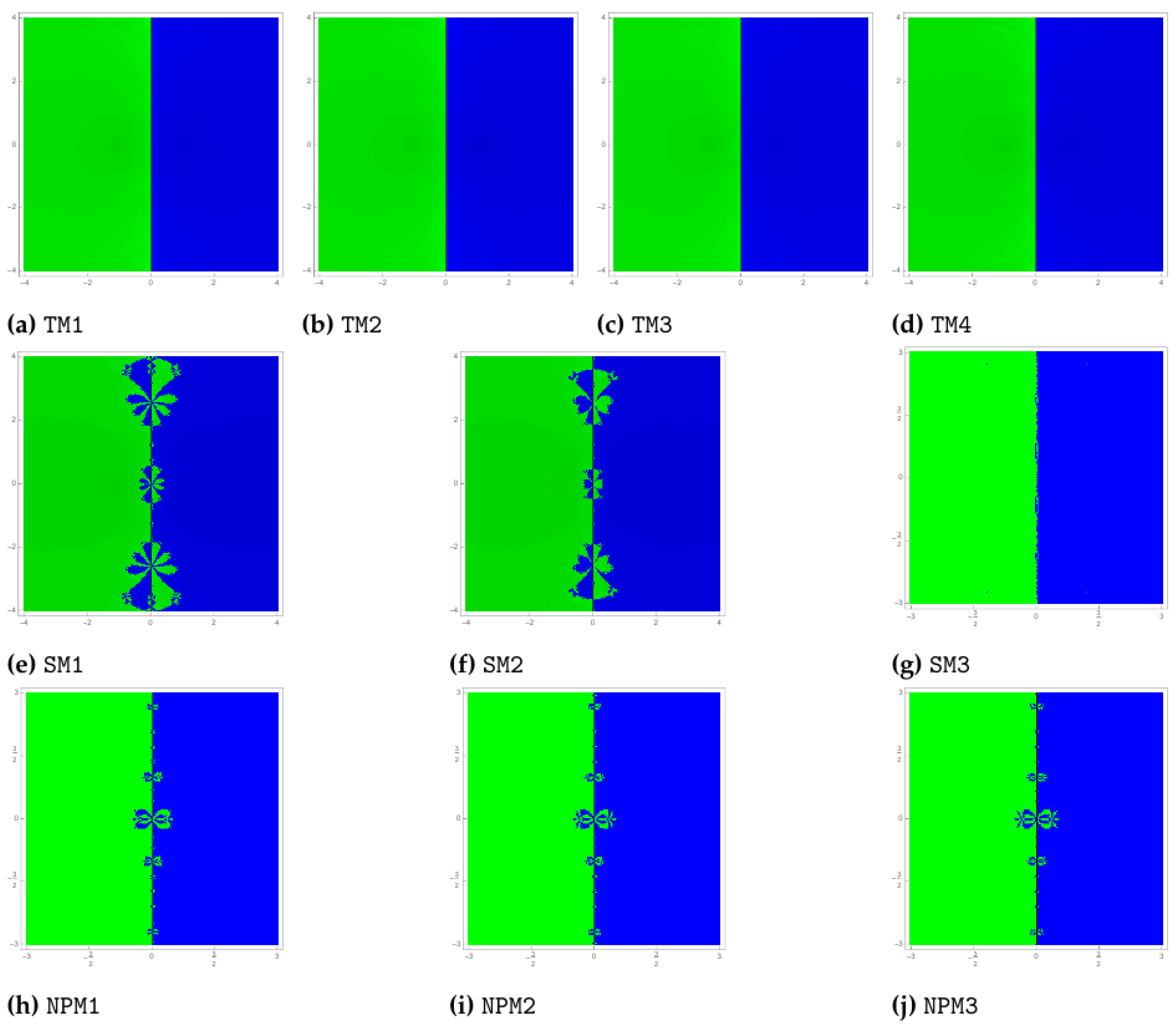
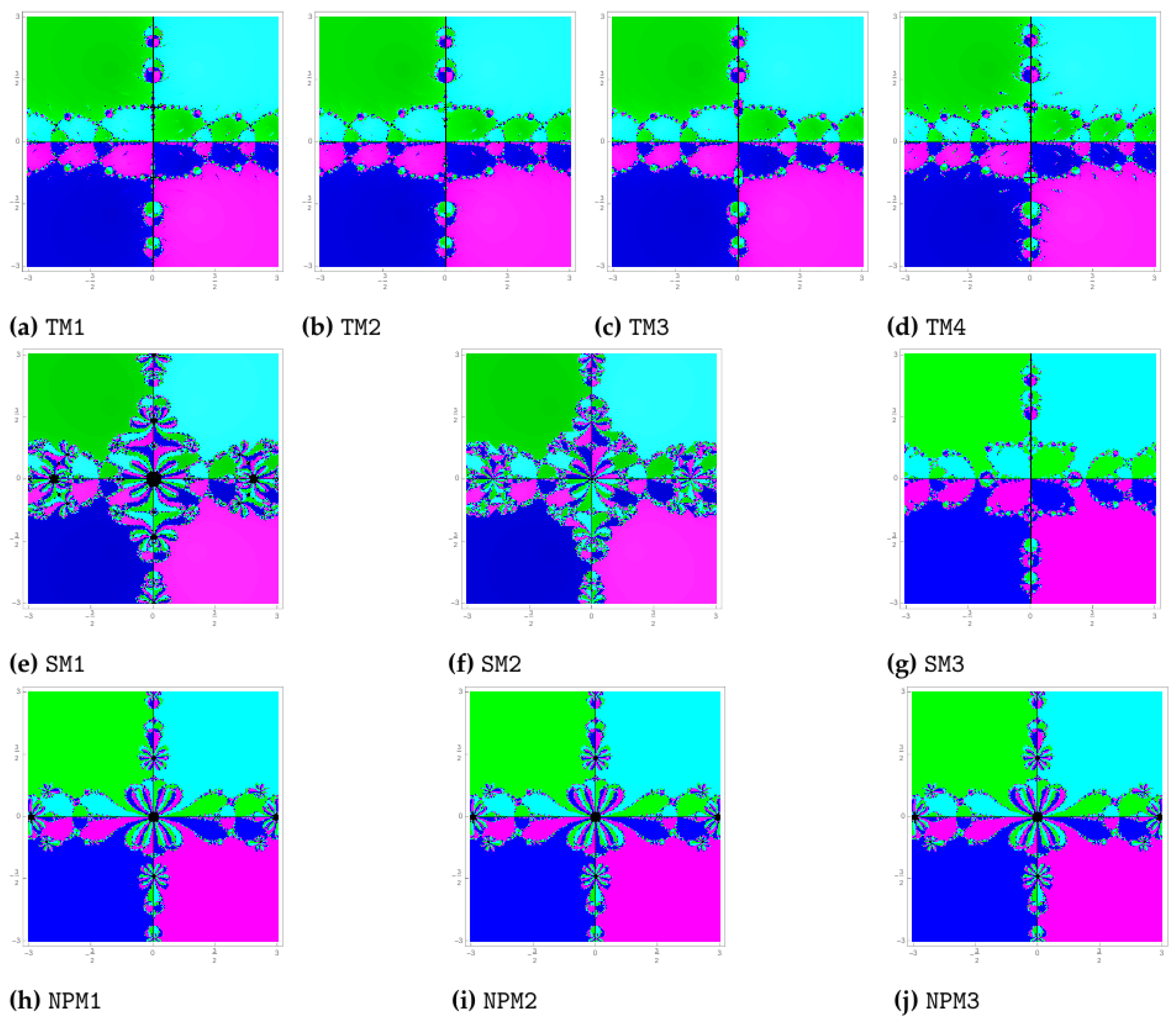
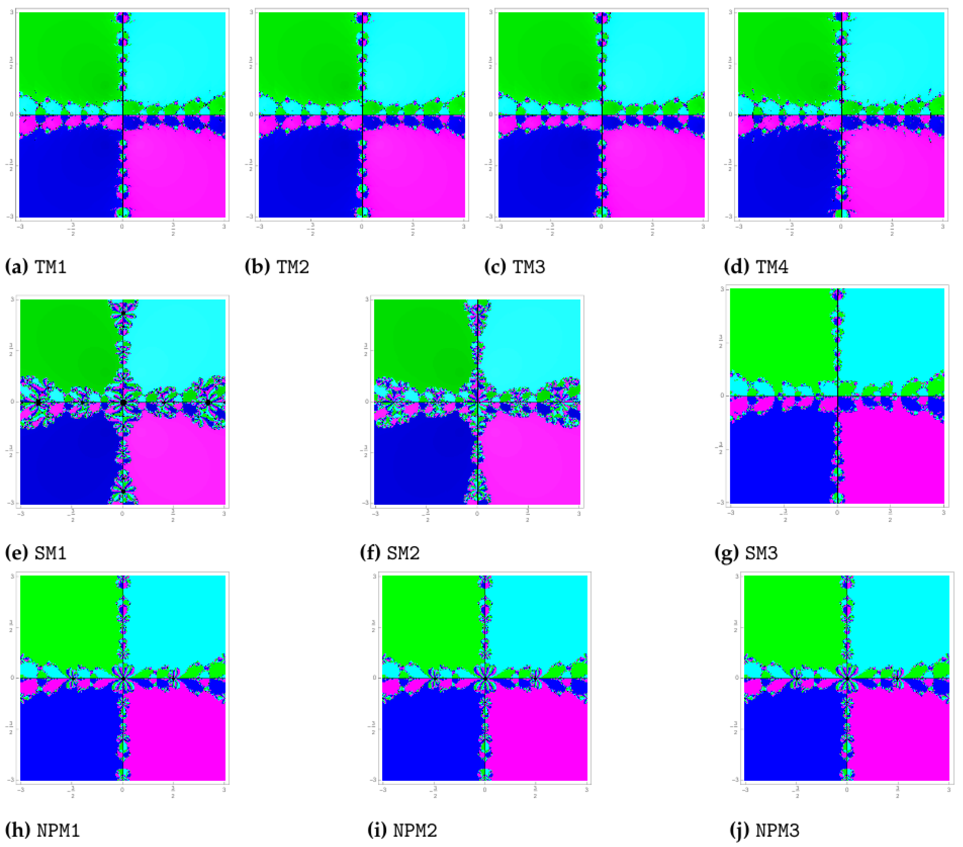
Problem 1.

Let us assume the polynomial $g_1\left(w\right)={(w^2-1)}^3$, having zeros $w=1,-1$ with multiplicity 3. Distribute the colours blue and green among each starting point in the basins of attraction of roots $-1$ and $1,$ respectively. Figure 1 shows the basins that were obtained for the methods TM1, TM2, TM3, TM4, SM1, SM2, SM3, NPM1, NPM2 and NPM3. From Figure 1, one can easily observe that the methods TM1, TM2, TM3 and TM4 divide the complex plane into two equal halves without any disturbance in the regions, but in case of the methods SM1, SM2, SM3, NPM1, NPM2 and NPM3, the complex plane is divided into two equal halves, which have disturbances. Therefore, the basins of attraction for the proposed methods, TM1, TM2, TM3 and TM4, are more stable than those for SM1, SM2, SM3, NPM1, NPM2 and NPM3. Among the newly proposed methods, all performed equally well.

Problem 2.

Now, consider the polynomial $g_2\left(w\right)={(w^4+4w^2+16)}^2$, having zeros $w=1+\sqrt{3}i,1-\sqrt{3}i,-1+\sqrt{3}i,-1-\sqrt{3}i$ with multiplicity $2.$ We have assigned the colors blue, green, magenta and cyan for each initial point in the basins of attraction of zeros $1+\sqrt{3}i,1-\sqrt{3}i,-1+\sqrt{3}i,-1-\sqrt{3}i,$ respectively. Figure 2 displays the basins created using the techniques TM1, TM2, TM3, TM4, SM1, SM2, SM3, NPM1, NPM2 and NPM3. Black spots in Figure 2 show the points which are not convergent to any of the roots. It is clear from Figure 2 that the convergence area is more for methods TM1, TM2, TM3, TM4 and SM3 as compared to the methods SM1, SM2, NPM1, NPM2 and NPM3. Furthermore, it can be seen that the new proposed methods, SM2 and SM3, do not contain any black spots which indicate the divergent points.

Problem 3.

Consider the polynomial $g_3\left(w\right)={(w^4+w^2+1)}^2.$ The roots of this polynomial are $w=\frac{1-\sqrt{3}i}{2}$, $\frac{1+\sqrt{3}i}{2}$, $\frac{-1-\sqrt{3}i}{2}$ and $\frac{-1+\sqrt{3}i}{2}$ with multiplicity $2.$ Assign the colours green, blue, cyan, and magenta to each initial point on the roots $\frac{1-\sqrt{3}i}{2},\frac{1+\sqrt{3}i}{2},\frac{-1-\sqrt{3}i}{2}$ and $\frac{-1+\sqrt{3}i}{2}.$ It is observed from Figure 3 that the proposed methods TM1, TM2, TM3 and TM4, as well as the method SM3, are adequate to converge to all the roots, and the divergent points occur in case of the methods SM1, SM2, NPM1, NPM2 and NPM3.

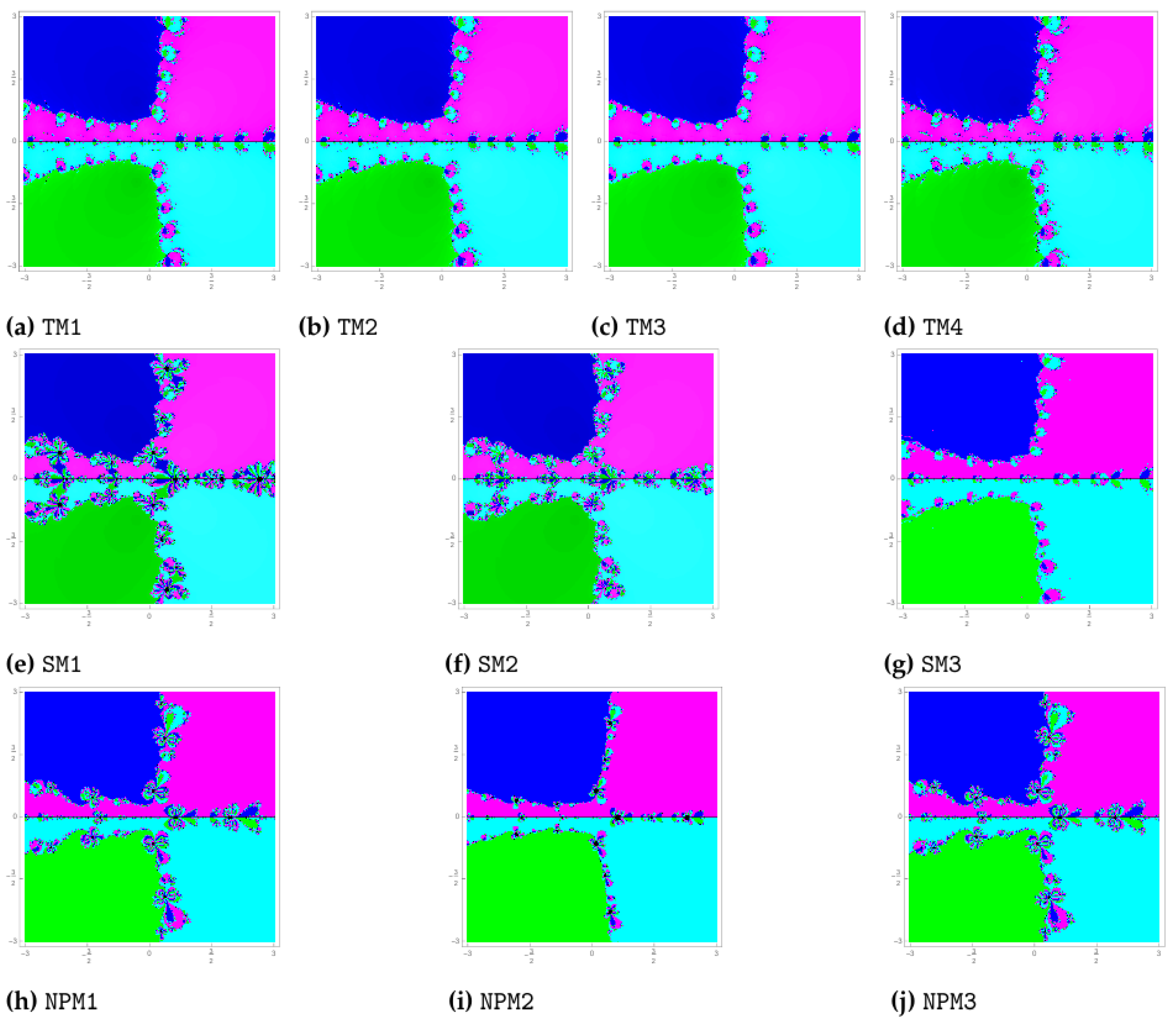
Problem 4.

The fourth polynomial we consider is $g_4\left(w\right)={(w^4-w^3+w^2-w+1)}^3.$ For this polynomial, $w=e^{\frac{\pi i}{5}}$, $e^{\frac{-\pi i}{5}}$, $e^{\frac{3\pi i}{5}}$ and $e^{\frac{-3\pi i}{5}}$ are the roots of the polynomial with multiplicity $3.$ We assign the colors to each initial guess of zero $e^{\frac{\pi i}{5}}$, $e^{\frac{-\pi i}{5}}$, $e^{\frac{3\pi i}{5}}$ and $e^{\frac{-3\pi i}{5}}$ as green, blue, cyan and magenta, respectively. It is observed from Figure 4 that the methods TM1, TM2, TM3, TM4 and SM3 do not contain any black spots, but the methods SM1, SM2, NPM1, NPM2 and NPM3 do contain them, which means that the methods TM1, TM2, TM3, TM4 and SM3 have performed better than the methods SM1, SM2, NPM1, NPM2 and NPM3.

As is visible in all figures, the basins of attraction possess reflection symmetry, and one can even go further to provide a proof for their symmetry [42], while in other instances [3] the behavior was identified as near to symmetric.

5. Numerical Results

The convergence of the newly generated methods is ensured in this section, numerically. Some nonlinear problems are solved by the newly generated methods. Other existing schemes mentioned in the previous section are also considered for comparison.

Mathematica programming software [33] is used to bring off the computational work. The numerical results are summarized in tabular form. The table embraces the number of iterations necessary to procure the root with finishing benchmark $|{\mathtt{x}}_{t+1}-{\mathtt{x}}_t|+\left|f\left({\mathtt{x}}_t\right)\right|<{10}^{-200}$ and estimated error $|{\mathtt{x}}_{t+1}-{\mathtt{x}}_t|$ in the last three iterations, residual error of the considered function $\left|f\left({\mathtt{x}}_t\right)\right|$ and computational order of convergence (COC), by exerting the formula:

$$COC=\frac{log\left|\frac{{\mathtt{x}}_{t+2}-\alpha }{{\mathtt{x}}_{t+1}-\alpha }\right|}{log\left|\frac{{\mathtt{x}}_{t+1}-\alpha }{{\mathtt{x}}_t-\alpha }\right|},\mathrm{where}t=1,2,\dots$$

(28)

The CPU running time is also presented in numerical results. For all the numerical computations, we have used Mathematica 12.0 programming software on Windows 10 on Intel Core i3. The problems considered for comparison are mentioned in

Table 2. Test functions.

Test Functions	Root	p	${\mathtt{x}}_0$
$f_1\left(\mathtt{x}\right)={\left({\mathtt{sin}}^2\mathtt{x}-{\mathtt{x}}^2+1\right)}^2$	1.4044916	2	2
$f_2\left(\mathtt{x}\right)={\mathtt{x}}^3-5.22{\mathtt{x}}^2+9.0825\mathtt{x}-5.2675$	1.7500000	2	2.2
$f_3\left(\mathtt{x}\right)={(\mathtt{x}-2)}^{15}{(\mathtt{x}-4)}^5{(\mathtt{x}-3)}^{10}{(\mathtt{x}-1)}^{20}$	1.0000000	20	0.7
$f_4\left(\mathtt{x}\right)={\mathtt{x}}^9-29{\mathtt{x}}^8+349{\mathtt{x}}^7-2261{\mathtt{x}}^6+8455{\mathtt{x}}^5-17663{\mathtt{x}}^4+15927{\mathtt{x}}^3+6993{\mathtt{x}}^2-24732\mathtt{x}+12960$	3.0000000	4	2.5
$f_5\left(\mathtt{x}\right)={[{(\mathtt{x}-1)}^3-1]}^{50}$	2.0000000	50	2.1

. For our methods, in all the problems we have taken $a=-1.$

The computational results in

Table 3. Computational results for function $f_1\left(\mathtt{x}\right)$.

Methods	t	$\left|{\mathit{e}}_{\mathit{t}-2}\right|$	$\left|{\mathit{e}}_{\mathit{t}-1}\right|$	$\left|{\mathit{e}}_{\mathit{t}}\right|$	$\left|\mathit{f}\left({\mathtt{x}}_{\mathit{t}+1}\right)\right|$	COC	CPU Time
TM1	5	$9.65\times {10}^{-12}$	$5.42\times {10}^{-56}$	$3.03\times {10}^{-277}$	$1.66\times {10}^{-2765}$	5.00000	0.00186139
TM2	5	$1.21\times {10}^{-11}$	$1.87\times {10}^{-55}$	$1.64\times {10}^{-274}$	$4.44\times {10}^{-2738}$	5.00000	0.00216832
TM3	5	$1.57\times {10}^{-11}$	$7.36\times {10}^{-55}$	$1.67\times {10}^{-271}$	$6.13\times {10}^{-2708}$	5.00000	0.00231683
TM4	5	$1.87\times {10}^{-12}$	$6.12\times {10}^{-60}$	$2.32\times {10}^{-297}$	$2.00\times {10}^{-2967}$	5.00000	0.00247525
SM1	5	$6.71\times {10}^{-11}$	$1.90\times {10}^{-51}$	$3.48\times {10}^{-254}$	$3.11\times {10}^{-2534}$	5.00000	0.00279208
SM2	5	$1.17\times {10}^{-10}$	$3.82\times {10}^{-50}$	$1.45\times {10}^{-247}$	$8.09\times {10}^{-2468}$	5.00000	0.00278218
SM3	5	$5.76\times {10}^{-11}$	$8.90\times {10}^{-52}$	$7.82\times {10}^{-256}$	$1.03\times {10}^{-2550}$	5.00000	0.00263366
NPM1	5	$2.83\times {10}^{-15}$	$3.23\times {10}^{-88}$	$7.21\times {10}^{-526}$	$4.85\times {10}^{-6302}$	6.00000	0.00279208
NPM2	5	$2.83\times {10}^{-15}$	$3.23\times {10}^{-88}$	$7.21\times {10}^{-526}$	$4.85\times {10}^{-6302}$	6.00000	0.00279208
NPM3	5	$2.83\times {10}^{-15}$	$3.23\times {10}^{-88}$	$7.21\times {10}^{-526}$	$4.85\times {10}^{-6302}$	6.00000	0.00279208

and

Table 4. Computational results for function $f_2\left(\mathtt{x}\right)$.

Methods	t	$\left|{\mathit{e}}_{\mathit{t}-2}\right|$	$\left|{\mathit{e}}_{\mathit{t}-1}\right|$	$\left|{\mathit{e}}_{\mathit{t}}\right|$	$\left|\mathit{f}\left({\mathtt{x}}_{\mathit{t}+1}\right)\right|$	COC	CPU Time
TM1	6	$4.66\times {10}^{-12}$	$5.07\times {10}^{-52}$	$7.73\times {10}^{-252}$	$1.22\times {10}^{-2502}$	5.00000	0.00154455
TM2	6	$5.77\times {10}^{-12}$	$1.57\times {10}^{-51}$	$2.31\times {10}^{-249}$	$7.59\times {10}^{-2478}$	5.00000	0.00170297
TM3	6	$7.45\times {10}^{-12}$	$5.92\times {10}^{-51}$	$1.87\times {10}^{-246}$	$1.02\times {10}^{-2448}$	5.00000	0.00138614
TM4	6	$1.29\times {10}^{-12}$	$5.41\times {10}^{-55}$	$7.17\times {10}^{-267}$	$2.57\times {10}^{-2653}$	5.00000	0.00169307
SM1	6	$3.21\times {10}^{-11}$	$1.31\times {10}^{-47}$	$1.46\times {10}^{-229}$	$2.01\times {10}^{-2279}$	5.00000	0.00215842
SM2	6	$5.73\times {10}^{-11}$	$2.87\times {10}^{-46}$	$8.98\times {10}^{-223}$	$2.18\times {10}^{-2211}$	5.00000	0.00262376
SM3	6	$2.65\times {10}^{-11}$	$5.00\times {10}^{-48}$	$1.21\times {10}^{-231}$	$3.03\times {10}^{-2300}$	5.00000	0.00231683
NPM1	6	$1.48\times {10}^{-18}$	$1.03\times {10}^{-100}$	$1.16\times {10}^{-593}$	$1.72\times {10}^{-7103}$	6.00000	0.00232673
NPM2	6	$1.48\times {10}^{-18}$	$1.03\times {10}^{-100}$	$1.16\times {10}^{-593}$	$1.72\times {10}^{-7103}$	6.00000	0.00247525
NPM3	6	$1.48\times {10}^{-18}$	$1.03\times {10}^{-100}$	$1.16\times {10}^{-593}$	$1.72\times {10}^{-7103}$	6.00000	0.00200990

show that the methods NPM1, NPM2 and NPM3 have the best residuals, but the major drawback of these methods is that they do not retain their order of convergence. Therefore, our proposed methods have performed better and possess lower residual error as well as low CPU-time for functions $f_1\left(\mathtt{x}\right)$ and $f_2\left(\mathtt{x}\right)$. They also preserve their fifth order of convergence. The numerical data for the function $f_3\left(\mathtt{x}\right)$ shown in

Table 5. Computational results for function $f_3\left(\mathtt{x}\right)$.

Methods	t	$\left|{\mathit{e}}_{\mathit{t}-2}\right|$	$\left|{\mathit{e}}_{\mathit{t}-1}\right|$	$\left|{\mathit{e}}_{\mathit{t}}\right|$	$\left|\mathit{f}\left({\mathtt{x}}_{\mathit{t}+1}\right)\right|$	COC	CPU Time
TM1	5	$1.52\times {10}^{-14}$	$2.00\times {10}^{-69}$	$7.74\times {10}^{-344}$	$1.03\times {10}^{-34298}$	5.00000	0.00139604
TM2	5	$2.12\times {10}^{-14}$	$1.15\times {10}^{-68}$	$5.39\times {10}^{-340}$	$1.13\times {10}^{-33913}$	5.00000	0.00139604
TM3	5	$3.08\times {10}^{-14}$	$8.08\times {10}^{-68}$	$9.98\times {10}^{-336}$	$3.42\times {10}^{-33486}$	5.00000	0.00108911
TM4	5	$1.46\times {10}^{-15}$	$7.05\times {10}^{-75}$	$1.84\times {10}^{-371}$	$2.49\times {10}^{-37068}$	5.00000	0.00154455
SM1	5	$2.29\times {10}^{-13}$	$3.26\times {10}^{-63}$	$1.92\times {10}^{-312}$	$9.26\times {10}^{-31153}$	5.00000	0.00262376
SM2	5	$4.77\times {10}^{-13}$	$1.62\times {10}^{-61}$	$7.34\times {10}^{-304}$	$2.06\times {10}^{-30292}$	5.00000	0.00247525
SM3	5	$1.84\times {10}^{-13}$	$1.08\times {10}^{-63}$	$7.68\times {10}^{-315}$	$1.82\times {10}^{-31392}$	5.00000	0.00171683
NPM1	Div	−	−	−	−	−	−
NPM2	Div	−	−	−	−	−	−
NPM3	Div	−	−	−	−	−	−

Here, Div means divergent.

demonstrate that TM4 performs better than the existing methods, with low error and precise result estimations. Further, the elapsed CPU time is minimal in the case of TM3. The numerical results obtained for function $f_4\left(\mathtt{x}\right)$ are shown in

Table 6. Computational results for function $f_4\left(\mathtt{x}\right)$.

Methods	t	$\left|{\mathit{e}}_{\mathit{t}-2}\right|$	$\left|{\mathit{e}}_{\mathit{t}-1}\right|$	$\left|{\mathit{e}}_{\mathit{t}}\right|$	$\left|\mathit{f}\left({\mathtt{x}}_{\mathit{t}+1}\right)\right|$	COC	CPU Time
TM1	5	$9.88\times {10}^{-24}$	$2.43\times {10}^{-117}$	$2.19\times {10}^{-585}$	$2.27\times {10}^{-11698}$	5.00000	0.00216832
TM2	5	$1.02\times {10}^{-23}$	$2.91\times {10}^{-117}$	$5.48\times {10}^{-585}$	$2.26\times {10}^{-11690}$	5.00000	0.00200990
TM3	5	$1.05\times {10}^{-23}$	$3.48\times {10}^{-117}$	$1.37\times {10}^{-584}$	$2.22\times {10}^{-11682}$	5.00000	0.00247525
TM4	5	$8.10\times {10}^{-24}$	$7.87\times {10}^{-118}$	$6.84\times {10}^{-588}$	$1.05\times {10}^{-11748}$	5.00000	0.00263366
SM1	5	$1.40\times {10}^{-23}$	$1.75\times {10}^{-116}$	$5.27\times {10}^{-581}$	$2.31\times {10}^{-11610}$	5.00000	0.00278218
SM2	5	$1.64\times {10}^{-23}$	$4.13\times {10}^{-116}$	$4.26\times {10}^{-579}$	$4.79\times {10}^{-11572}$	5.00000	0.00294059
SM3	5	$1.40\times {10}^{-23}$	$1.71\times {10}^{-116}$	$4.76\times {10}^{-581}$	$3.02\times {10}^{-11611}$	5.00000	0.00340595
NPM1	5	$2.50\times {10}^{-18}$	$3.16\times {10}^{-90}$	$1.02\times {10}^{-449}$	$1.21\times {10}^{-8984}$	5.00000	0.00309901
NPM2	5	$2.70\times {10}^{-18}$	$4.94\times {10}^{-90}$	$1.00\times {10}^{-448}$	$1.18\times {10}^{-8964}$	5.00000	0.00324752
NPM3	5	$2.90\times {10}^{-18}$	$7.52\times {10}^{-90}$	$8.78\times {10}^{-448}$	$1.04\times {10}^{-8945}$	5.00000	0.00308911

. One can observe that each scheme has extremely high precision, with the lowest residual calculated by TM4.

Table 7. Computational results for function $f_5\left(\mathtt{x}\right)$.

Methods	t	$\left|{\mathit{e}}_{\mathit{t}-2}\right|$	$\left|{\mathit{e}}_{\mathit{t}-1}\right|$	$\left|{\mathit{e}}_{\mathit{t}}\right|$	$\left|\mathit{f}\left({\mathtt{x}}_{\mathit{t}+1}\right)\right|$	COC	CPU Time
TM1	5	$1.11\times {10}^{-25}$	$2.25\times {10}^{-125}$	$7.74\times {10}^{-624}$	$1.96\times {10}^{-155748}$	5.00000	0.00200990
TM2	5	$2.01\times {10}^{-25}$	$4.90\times {10}^{-124}$	$4.26\times {10}^{-617}$	$8.03\times {10}^{-154061}$	5.00000	0.00170301
TM3	5	$3.61\times {10}^{-25}$	$1.02\times {10}^{-122}$	$1.82\times {10}^{-610}$	$1.64\times {10}^{-152400}$	5.00000	0.00200990
TM4	5	$4.50\times {10}^{-28}$	$6.15\times {10}^{-138}$	$2.92\times {10}^{-687}$	$2.36\times {10}^{-171634}$	5.00000	0.00170297
SM1	5	$1.08\times {10}^{-23}$	$4.79\times {10}^{-115}$	$8.42\times {10}^{-572}$	$2.36\times {10}^{-142719}$	5.00000	0.00247525
SM2	5	$3.65\times {10}^{-23}$	$2.79\times {10}^{-112}$	$7.39\times {10}^{-558}$	$6.33\times {10}^{-139228}$	5.00000	0.00231683
SM3	5	$8.89\times {10}^{-24}$	$1.85\times {10}^{-115}$	$7.26\times {10}^{-574}$	$1.87\times {10}^{-143235}$	5.00000	0.00757426
NPM1	Div	−	−	−	−	−	−
NPM2	Div	−	−	−	−	−	−
NPM3	Div	−	−	−	−	−	−

Here, Div means divergent.

shows the numerical results of the methods for function $f_5\left(\mathtt{x}\right)$. The best performer for this function is TM4. Furthermore, it is worth mentioning here that the methods NPM1–NPM3 do not converge to the required root for the problems $f_3\left(\mathtt{x}\right)$ and $f_5\left(\mathtt{x}\right)$, or we can say that they are divergent for these problems.

6. Concluding Remarks

We have introduced a new multi-point iterative algorithm that can solve nonlinear equations having multiple zeros. The scheme is based on the weight function approach. Per iteration, the presented scheme requires two assessments of functions and two assessments of its derivatives to achieve the fifth order convergence. Some special cases of the new family are also presented. The presented basins of attraction have confirmed that the performance of the new methods is on par with or better than the established schemes in the literature. The theoretical results proved in the paper regarding the order of convergence are verified through various numerical examples. A comparison with the existing methods is also made. The results obtained have once again proved the robustness of the new schemes. Moreover, the CPU time is also evaluated, which is lesser for the newly proposed schemes. In a nutshell, we can say that the new methods have performed better than the existing methods in terms of basins of attraction, the number of iterations required to converge to the root, residual errors and CPU-time for the considered problems.

References

1. Kumar, D.; Sharma, J.R.; Cesarano, C. One-Point Optimal Family of Multiple Root Solvers of Second-Order. Mathematics 2019, 7, 655. [Google Scholar] [CrossRef] [Green Version]
2. Sharma, J.R.; Kumar, S.; Jäntschi, L. On Derivative Free Multiple-Root Finders with Optimal Fourth Order Convergence. Mathematics 2020, 8, 1091. [Google Scholar] [CrossRef]
3. Alharbey, R.A.; Kansal, M.; Behl, R.; Machado, J.A.T. Efficient Three-Step Class of Eighth-Order Multiple Root Solvers and Their Dynamics. Symmetry 2019, 11, 837. [Google Scholar] [CrossRef] [Green Version]
4. Sharma, J.R.; Kumar, S.; Jäntschi, L. On a Class of Optimal Fourth Order Multiple Root Solvers without Using Derivatives. Symmetry 2019, 11, 1452. [Google Scholar] [CrossRef] [Green Version]
5. Sharma, J.R.; Kumar, D.; Cattani, C. An Efficient Class of Weighted-Newton Multiple Root Solvers with Seventh Order Convergence. Symmetry 2019, 11, 1054. [Google Scholar] [CrossRef] [Green Version]
6. Sharma, J.R.; Kumar, D.; Argyros, I.K. An Efficient Class of Traub-Steffensen-Like Seventh Order Multiple-Root Solvers with Applications. Symmetry 2019, 11, 518. [Google Scholar] [CrossRef] [Green Version]
7. Chun, C.; Neta, B. A Third-Order Modification of Newton’s Method for Multiple Roots. Appl. Math. Comput. 2009, 211, 474–479. [Google Scholar] [CrossRef] [Green Version]
8. Hansen, E.; Patrick, M. A family of root finding methods. Numer. Math. 1977, 27, 257–269. [Google Scholar] [CrossRef]
9. Neta, B. New third order nonlinear solvers for multiple roots. Appl. Math. Comput. 2008, 202, 162–170. [Google Scholar] [CrossRef] [Green Version]
10. Osada, N. An optimal multiple root finding method of order three. J. Comput. Appl. Math. 1994, 51, 131–133. [Google Scholar] [CrossRef]
11. Sharma, J.R.; Sharma, R. Modified Chebyshev–Halley Type Method and Its Variants for Computing Multiple Roots. Numer. Algorithms 2012, 61, 567–578. [Google Scholar] [CrossRef]
12. Schröder, E. Über unendlich viele Algorithmen zur Auflösung der Gleichungen. Math. Ann. 1870, 2, 317–365. [Google Scholar] [CrossRef] [Green Version]
13. Zhou, X.; Chen, X.; Song, Y. Families of third and fourth order methods for multiple roots of nonlinear equations. Appl. Math. Comput. 2013, 219, 6030–6038. [Google Scholar] [CrossRef]
14. Geum, Y.H.; Kim, Y.I.; Neta, B. A class of two-point sixth-order multiple-zero finders of modified double-Newton type and their dynamics. Appl. Math. Comput. 2015, 270, 387–400. [Google Scholar] [CrossRef] [Green Version]
15. Geum, Y.H.; Kim, Y.I.; Neta, B. A sixth-order family of three-point modified Newton-like multiple-root finders and the dynamics behind their extraneous fixed points. Appl. Math. Comput. 2016, 283, 120–140. [Google Scholar] [CrossRef] [Green Version]
16. Behl, R.; Cordero Barbero, A.; Motsa, S.S.; Torregrosa Sánchez, J.R. An eighth-order family of optimal multiple root finders and its dynamics. Numer. Algorithms 2018, 77, 1249–1272. [Google Scholar] [CrossRef] [Green Version]
17. Li, S.; Liao, X.; Cheng, L. A new fourth-order iterative method for finding multiple roots of nonlinear equations. Appl. Math. Comput. 2009, 215, 1288–1292. [Google Scholar]
18. Zhou, X.; Chen, X.; Song, Y. Constructing higher-order methods for obtaining the multiple roots of nonlinear equations. Comput. Appl. Math. 2011, 235, 4199–4206. [Google Scholar] [CrossRef] [Green Version]
19. Behl, R.; Kansal, M.; Salimi, M. Modified King’s Family for Multiple Zeros of Scalar Nonlinear Functions. Mathematics 2020, 8, 827. [Google Scholar] [CrossRef]
20. Kansal, M.; Cordero, A.; Torregrosa Sánchez, J.R.; Bhalla, S. A stable class of modified Newton-like methods for multiple roots and their dynamics. Int. J. Nonlinear Sci. Numer. Simul. 2020, 21, 603–621. [Google Scholar] [CrossRef]
21. Rani, L.; Soleymani, F.; Kansal, M.; Kumar Nashine, H. An optimized Chebyshev–Halley type family of multiple solvers: Extensive analysis and applications. Math. Methods Appl. Sci. 2022, 8699. [Google Scholar] [CrossRef]
22. Sharma, J.R. A family of third-order methods to solve nonlinear equations by quadratic curves approximation. Appl. Math. Comput. 2007, 184, 210–215. [Google Scholar] [CrossRef]
23. Sharma, J.R. A family of methods for solving nonlinear equations using quadratic interpolation. Comput. Math. Appl. 2004, 48, 709–714. [Google Scholar] [CrossRef] [Green Version]
24. Cordero, A.; Hueso, J.L.; Martinez, E.; Torregrosa, J.R. A new technique to obtain derivative-free optimal iterative methods for solving nonlinear equations. J. Comput. Appl. Math. 2013, 252, 95–102. [Google Scholar] [CrossRef]
25. Ostrowski, A.M. Solution of Equations and Systems of Equations; Academic Press: New York, NY, USA, 1966. [Google Scholar]
26. Behl, R. A Derivative Free Fourth-Order Optimal Scheme for Applied Science Problems. Mathematics 2022, 10, 1372. [Google Scholar] [CrossRef]
27. Abbasbandy, S. Improving Newton-Raphson method for nonlinear equations by modified Adomian decomposition method. Appl. Math. Comput. 2003, 145, 887–893. [Google Scholar] [CrossRef]
28. Babajee, D.K.R.; Cordero, A.; Soleymani, F.; Torregrosa, J.R. On improved three-step schemes with high efficiency index and their dynamics. Numer. Algorithms 2014, 65, 153–169. [Google Scholar] [CrossRef]
29. Behl, R.; Bhalla, S.; Magreñán, Á.A.; Moysi, A. An Optimal Derivative Free Family of Chebyshev–Halley’s Method for Multiple Zeros. Mathematics 2021, 9, 546. [Google Scholar] [CrossRef]
30. Artidiello, S.; Cordero, A.; Torregrosa, J.R.; Vassileva, M.P. Multidimensional generalization of iterative methods for solving nonlinear problems by means of weight-function procedure. Appl. Math. Comput. 2015, 268, 1064–1071. [Google Scholar] [CrossRef] [Green Version]
31. Cordero, A.; Iqbal, S.; Torregrosa, J.R.; Zafar, F. New Iterative Schemes to Solve Nonlinear Systems with Symmetric Basins of Attraction. Symmetry 2022, 14, 1742. [Google Scholar] [CrossRef]
32. Chanu, W.H.; Panday, S.; Thangkhenpau, G. Development of Optimal Iterative Methods with Their Applications and Basins of Attraction. Symmetry 2022, 14, 2020. [Google Scholar] [CrossRef]
33. Wolfram, S. The Mathematica Book, 5th ed.; Wolfram Media: Champaign, IL, USA, 2003. [Google Scholar]
34. Said Solaiman, O.; Hashim, I. Efficacy of Optimal Methods for Nonlinear Equations with Chemical Engineering Applications. Math. Probl. Eng. 2019, 11, 1–11. [Google Scholar] [CrossRef] [Green Version]
35. Said Solaiman, O.; Hashim, I. An iterative scheme of arbitrary odd order and its basins of attraction for nonlinear systems. Comput. Mater. Cont. 2021, 66, 1427–1444. [Google Scholar] [CrossRef]
36. Fatou, P. Sur les équations fonctionelles. Bull. Soc. Math. France 1919, 47, 161–271. [Google Scholar] [CrossRef] [Green Version]
37. Julia, G.M. Mémoire sur l’itération des fonctions rationelles. J. Math. Pures Appl. 1918, 1, 47–246. [Google Scholar]
38. Sharma, J.R.; Arora, H. Some novel optimal eighth order derivative-free root solvers and their basins of attraction. Appl. Math. Comput. 2016, 284, 149–161. [Google Scholar] [CrossRef]
39. Kumar, S.; Bhagwan, J.; Jäntschi, L. Optimal Derivative-Free One-Point Algorithms for Computing Multiple Zeros of Nonlinear Equations. Symmetry 2022, 14, 1881. [Google Scholar] [CrossRef]
40. Sharma, J.R.; Arora, H. A Family of Fifth-Order Iterative Methods for Finding Multiple Roots of Nonlinear Equations. Numer. Anal. Appl. 2021, 14, 186–199. [Google Scholar] [CrossRef]
41. Henarita Chanu, W.; Panday, S.; Dwivedi, M. New Fifth Order Iterative Method for Finding Multiple Root of Nonlinear Function. Eng. Lett. 2021, 29, 942–947. [Google Scholar]
42. Bray, K.; Dwyer, J.; Barnard, R.W.; Williams, G.B. Fixed Points, Symmetries, and Bounds for Basins of Attraction of Complex Trigonometric Functions. Int. J. Math. Math. Sci. 2020, 2020, 1853467. [Google Scholar] [CrossRef]
Figure 1. Basins of attraction of TM1TM4, SM1SM3 and NPM1NPM3 for polynomial g 1 ( w ) .
Symmetry 15 00228 g001
Figure 2. Basins of attraction of TM1TM4, SM1SM3 and NPM1NPM3 for polynomial g 2 ( w ) .
Symmetry 15 00228 g002
Figure 3. Basins of attraction of TM1TM4, SM1SM3 and NPM1NPM3 for polynomial g 3 ( w ) .
Symmetry 15 00228 g003
Figure 4. Basins of attraction of TM1TM4, SM1SM3 and NPM1NPM3 for polynomial g 4 ( w ) .
Symmetry 15 00228 g004