Event-Triggered Sliding Mode Impulsive Control for Lower Limb Rehabilitation Exoskeleton Robot Gait Tracking

Abstract

Lower limb rehabilitation exoskeleton robots (LLRERs) play an important role in lower limb rehabilitation training and assistance walking for patients with lower limb movement disorders. In order to reduce and eliminate adverse effects on the accuracy of human motion gait tracking during walking with an LLRER, which is caused by the gravity and friction, the periodic ground shock force, and the human–exoskeleton interaction force, this paper proposes a feedforward–feedback hybrid control strategy of sliding mode impulsive control with gravity and friction compensation, based on the event-triggered mechanism of Lyapunov function. Firstly, to realize high-precision gait tracking with bounded error, some constraints on controller parameters are deduced by analyzing the Lyapunov-based stability. Secondly, the Zeno behavior of impulsive event triggers is excluded by the analysis of three different cases of the triggering time sequence. Finally, the effectiveness of the proposed hybrid controller is verified by the numerical simulation of the LLRER human–exoskeleton integrated system based on a three-link simplified model. It shows that an event-triggered sliding mode impulsive control strategy with gravity and friction compensation can achieve complete gait tracking with bounded error and has excellent dynamic performance under the constraints.

1. Introduction

Over the past decades, there have been more and more patients with lower limb hemiplegia, paraplegic, cerebral palsy, and limb movement disorders, caused by increasing traffic accidents, stroke, and population aging [1,2,3]. Consequently, the rehabilitation training and assistance walking of the elderly, disabled, and others with movement disorders has become a major social problem. Since the 1960s, after the first exoskeleton “Hardiman” was made in America, many different exoskeletons have been developed to try to solve the problem over the world, for example, BLEEX, ALEX, Lokomat, LOPES, Rewalk, Ekso, Rex, HAL, HULC, CUHK-EXO, and so on [4,5,6,7,8]. As an effective medical auxiliary intelligent device, lower limb rehabilitation exoskeleton robots (LLRERs) have been rapidly developed and widely used in many hospitals and families, and there is a huge market demand and development potential for LLRERs.

In order to make the movements more flexible and compliant and the gait trajectory more natural and stable, it is very important to realize high-precision human motion gait tracking of the LLRER human–exoskeleton integrated system [9,10]. So it has become a current research hotspot in the field of exoskeleton and orthoses and it has attracted considerable attention and the interest of many researchers around the world. The position feedback PD control is a common and simple method of human motion gait tracking, but it is difficult to perform PD parameter tuning due to the inaccurate dynamic model of the system [11]. To take the role of force or torque into account in gait tracking, accordingly, a force and position hybrid control method is formulated in [12,13]. However, some external disturbances and mechanical friction are undetectable by sensors, so it still cannot obtain the desired gait results. Consequently, the sliding mode control (SMC) method is introduced for its complete robustness to some uncertain factors, such as structural uncertainties, parameter uncertainties, and external disturbances [14,15]. Unfortunately, the high-frequency chatter caused by SMC is harmful to motors used for joint drivers. Furthermore, to decrease chatter in SMC, the sign function is replaced by a hyperbolic tangent function or sigmoid function, and some artificial intelligence algorithms are adopted [16,17,18,19]. Moreover, sensitivity amplify control (SAC) was first used in BLEEX, and a good tracking control effect can be obtained based only on an accurate dynamic model [5]. In recent years, new and effective means for flexible movement, admittance control, and impedance control are proposed and used in robots [20,21,22]. The core ideas of them are the same, to ensure some relationship between external force and position tracking error. In other words, they all belong to the force and position hybrid control method essentially. Because the gait trajectory of human motion is periodic and repetitive, iterative learning control (ILC) is extremely applicable [23,24]. Moreover, it does not rely on the precise mathematical model of the dynamic system, and it can reduce gait tracking errors significantly with only a few iterations. However, in the LLRER system, ILC is invalid for non-repetitive external disturbance.

Recently, with the rapid development of sensor technology, the human–robot cooperative control based on multi-sensor signals fusion technology is proposed to obtain perfect gait tracking, including plantar pressure sensor, angle position encoder, inertial measurement unit (IMU), and human physiological signals sensors, such as surface electromyogram (sEMG) [25,26], electroencephalogram (EEG), electrooculogram (EOG) [27,28], and brain–machine [29]. Obviously, there are too many signals and too much data in the above continuous system caused by periodic sampling called time-triggered control. Furthermore, in order to effectively reduce the number of sensor signals and decrease the amount of data sent in the communication network, event-triggered control is proposed and mainly applied in networked control systems. It was proven that event-triggered control can save the computational resources of the controller and the network bandwidth and reduce the energy consumption of the sensor network. The event-triggered SMC is widely used for its advantages [27,30]. Lately, impulsive control has developed rapidly due to its advantages such as simpler structure, stronger robustness, and lower control cost [31,32,33,34,35]. Specifically, compared with other control methods, the advantages and outstanding features of impulsive control can be summarized as follows: on the one hand, the impulsive controller is simple in structure and easy to implement. Only the linear feedback of the state signal is used as the impulsive control signal to realize the control of the impulsive system [36,37]. Therefore, it greatly reduces the requirements for sensors and communication technology, and consequently, it can be implemented at a low cost. On the other hand, impulsive control systems have strong robustness and are suitable for solving problems such as strong nonlinearity, parameter uncertainty, time delay, and random disturbance. In addition, impulsive control can provide an effective method to deal with systems that cannot continuously control. Last but not least, impulsive control reduces information redundancy and transmission delay and accelerates response speed [38,39]. As a result, impulsive control based on event-triggered mechanisms has received considerable attention due to its wide applications in fields such as communication networks, control technology, engineering sciences, and biology [40,41,42].

As we know, at the moment a user’s heel touches with the toe off the ground, the LLRER human–exoskeleton integrated system will be subjected to the external shock force and human–exoskeleton interaction force. Generally, they are regarded as time-varying and external random disturbances which cannot be accurately measured by sensors and have a bad influence on gait tracking but cannot be ignored [43]. In order to reduce and eliminate the adverse effects, this paper synthesizes the advantages of above several different control strategies and proposes the sliding mode impulse control based on the event-triggered mechanism [27,44]. By simulation verification, the proposed hybrid control strategy can achieve perfect gait tracking for the LLRER human–exoskeleton integrated system. The originalities and the novelties of the proposed control system are summarized as follows: (1) Although there are many control methods for exoskeleton robot trajectory tracking, our paper is the first time applying impulsive control to exoskeleton robots. (2) Although event-triggered control has been widely and maturely used in networked control systems and complex networks, there are few studies on its application to improve the accuracy of exoskeleton gait tracking. (3) Sliding mode control is a common nonlinear control method, but it is the first time to design a hybrid controller by combining the sliding mode control (SMC) with event-triggered impulsive control (ETIC) [45,46]. (4) In addition, in references [6,9,11,14], passive ankle joints are used, so the controllers are designed only based on the common dynamic model of the two-link manipulator; meanwhile, the friction is ignored in the dynamic model, which greatly reduces the accuracy of lower limb exoskeleton gait tracking. Moreover, a sinusoidal signal is used as the desired trajectory in [9,11,47], and it is different from the practical gait trajectory. However, different from the above, active ankle joints are used in our CUHK-EXO LLRER, and the dynamic model of the human–exoskeleton integrated not only includes the exoskeleton, but it also includes the human body mass inertia parameters and the Coulomb viscous friction model. Moreover, the walking gait of healthy humans is used as the desired trajectory for patients with lower limb movement disorders at the early stage of passive rehabilitation training.

The major contributions of this paper are as follows: (1) In order to reduce and eliminate adverse effects on the accuracy of gait tracking caused by the gravity and friction, the periodic ground shock force, and human–exoskeleton interaction force during a patient with lower limb disorder walking with an LLRER, the feedforward compensation control, impulsive control based on event-triggered mechanism, and sliding mode control are combined to design the controller of LLRER gait tracking. (2) Based on event-triggered sliding mode impulsive control, the constraints of gait tracking with bounded error and exclusion of Zeno behavior are derived and proved, respectively, and they are useful for the selection of the hybrid controller parameters.

The rest of this paper is organized as follows. In Section 2, some notations, definitions, and assumptions are provided, and the problem and the design of the hybrid controller are formulated. Our main results are proposed in Section 3, including Lyapunov-based stability analysis and Zeno behavior exclusion. A numerical simulation of a practical human–exoskeleton integrated system with the proposed hybrid controller is presented and results are discussed in Section 4. Finally, the paper is concluded in Section 5.

2. Models and Method

2.1. Notation

Let $\mathbb{R}$, ${\mathbb{R}}^{+}$, and ${\mathbb{Z}}^{+}$ denote the set of real numbers, positive real numbers, and positive integers, respectively. ${\mathbb{R}}^n$ is the n-dimensional real spaces with Euclidean norm, and ${\mathbb{R}}^{m\times n}$ represents $m\times n$ dimensional real space. In addition, $a\vee b$ is the maximum of a and b. The notation $A^T$ and $A^{-1}$ denote the transpose and inverse of matrix A, respectively. $diag[\cdots ]$ denotes a diagonal matrix. $\delta (t-t_k)$ is the Dirac delta function, it presents the impulsive effects due to impulsive action at instant $t_k$, and ${\{t_k,k\in {\mathbb{Z}}^{+}\}}_{k=1}^{\infty }$ is time sequence generated by the impulsive event-triggered mechanism (IETM). $I_3$ is the third-order identity matrix. $\lambda$ is the proportion coefficient and $\lambda >0$.

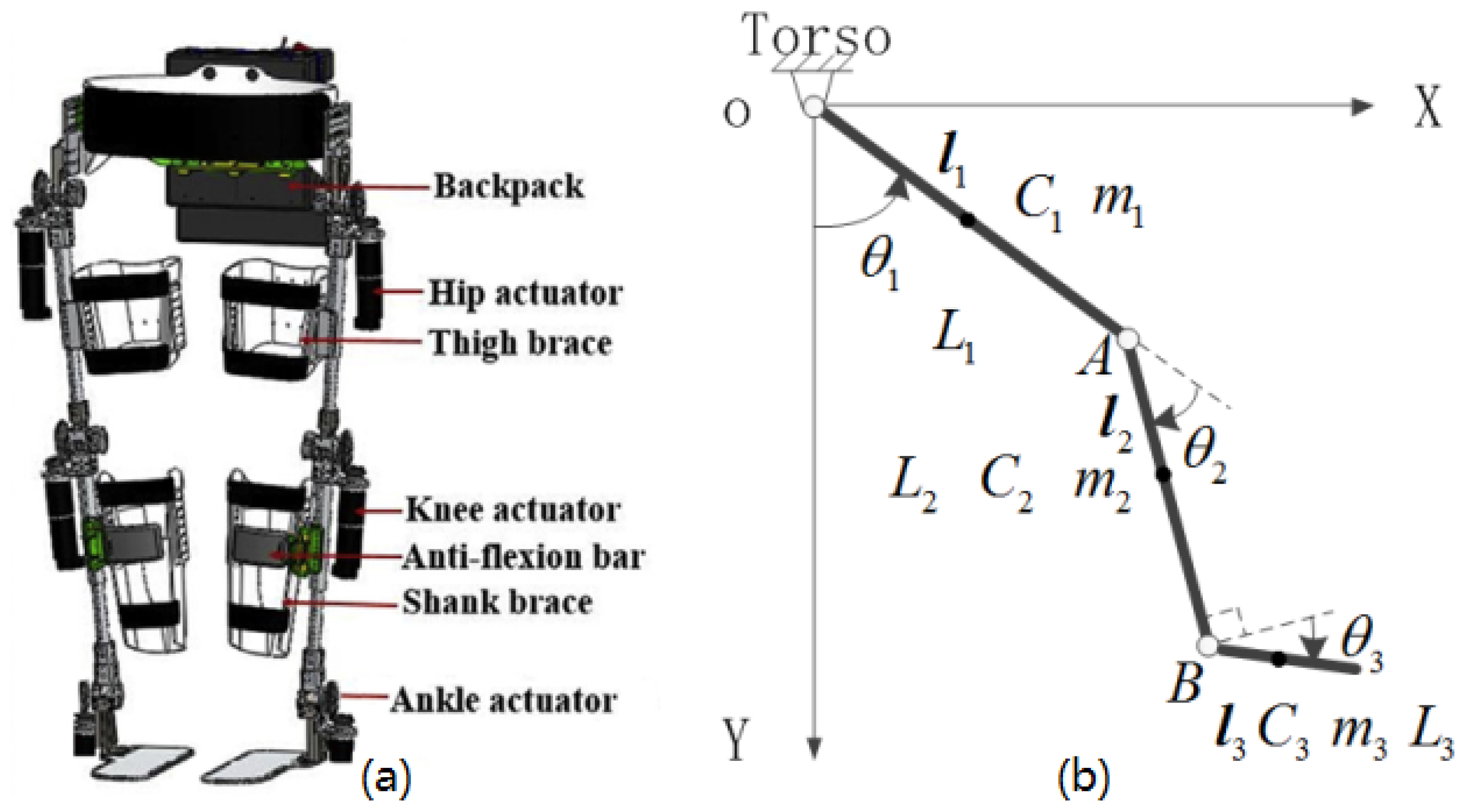
2.2. Dynamic Model of CUHK-EXO LLRER

Generally, the dynamic model of an articulated robot with revolute joints can be described by a Lagrangian system as follows [10,11,48]:

$$M(\theta )\ddot{\theta }+C(\theta ,\dot{\theta })\dot{\theta }+G\left(\theta \right)+F(\dot{\theta })=T+{\tau }_{\mathrm{d}}$$

(1)

where $\theta \in {\mathbb{R}}^n$ is the vector of generalized coordinate, $\dot{\theta }\in {\mathbb{R}}^n$ is the vector of generalized velocity, and $\ddot{\theta }\in {\mathbb{R}}^n$ is the vector of generalized acceleration. $M(\theta ),C(\theta ,\dot{\theta })\in {\mathbb{R}}^{n\times n}$ represent the symmetric positive-definite mass-inertia matrix and the Coriolis and centrifugal forces matrix, separately. $G(\theta ),F(\dot{\theta }),{\tau }_d,T\in {\mathbb{R}}^{n\times n}$ represent the gravity, Coulomb viscous force, external disturbance, and the output torque of joint actuator, respectively.

For the Lagrangian dynamic system (1), there are two fundamental properties, as follows [10,11].

 Property 1.

The matrix $\dot{M}(\theta )-2C(\theta ,\dot{\theta })$ is skew-symmetric, and it holds for arbitrary $x\in {\mathbb{R}}^n$

$$x^T(\dot{M}(\theta )-2C(\theta ,\dot{\theta }))x=0$$

(2)

 Property 2.

There exist three constants $M_1,M_2,k_c\in {\mathbb{R}}^{+}$ that are skew-symmetric and hold for arbitrary $x\in {\mathbb{R}}^n$, such that

$$M_1\le \parallel M(\theta )\parallel \le M_2,\parallel C(\theta ,\dot{\theta })\parallel \le k_c\parallel \dot{\theta }\parallel$$

(3)

As shown in Figure 1a, taking the CUHK-EXO as an example, the prototype of the wearable LLRER is developed by the Chinese University of Hong Kong (CUHK) research team and is called CUHK-EXO [10,11,24,49,50]. When a user is walking with LLRER for rehabilitation training, the two legs alternatively stand and swing in a gait cycle. To make the analysis of LLRER easier, the thigh, shank, and foot can be approximated as three different rigid bodies. So the swing leg can be simplified into a three-link structure as shown in Figure 1b. O stands for the position of the hip joint, A stands for the position of the knee hip joint, and B stands for the position of the ankle joint. $m_1$, $m_2$, and $m_3$ present the mass of the thigh, shank, and foot, separately. $L_1$, $L_2$, and $L_3$ are the lengths of body segments. $C_1$, $C_2$, and $C_3$ are the centers of mass (COMs) of them. $l_1$, $l_2$, and $l_3$ represent the distance from the joint position to the COM, separately. The inertia of different segments rotating around their COMs are represented by $I_1$, $I_2$, and $I_3$, respectively. ${\theta }_1$, ${\theta }_2$, and ${\theta }_3$ represent the angles of three joints. The angular ranges are defined as follows: ${\theta }_1\in [-30°,30°]$, ${\theta }_2\in [0°,60°]$, ${\theta }_3\in [-20°,20°]$. $\theta$, $\dot{\theta }$, and $\ddot{\theta }$ denote the position, angular velocity, and angular acceleration of the joints, respectively. $\theta \left(t\right)={\left[{\theta }_1\left(t\right){\theta }_2\left(t\right){\theta }_3\left(t\right)\right]}^T$ denotes the actual angles of the hip, knee, and ankle joints, as shown in Figure 1b. ${\theta }_d\left(t\right)={\left[{\theta }_{1d}\left(t\right){\theta }_{2d}\left(t\right){\theta }_{3d}\left(t\right)\right]}^T$ represents the time-varying desired joint angles of human motion during walking. Let $f_v$ and $f_c$ present the viscous friction coefficient and the Coulomb friction coefficient of Coulomb viscous friction, respectively.

For the three-link simplified model of the human–exoskeleton integrated system in Figure 1b, the dynamic model (1) can be written as in [10,11].

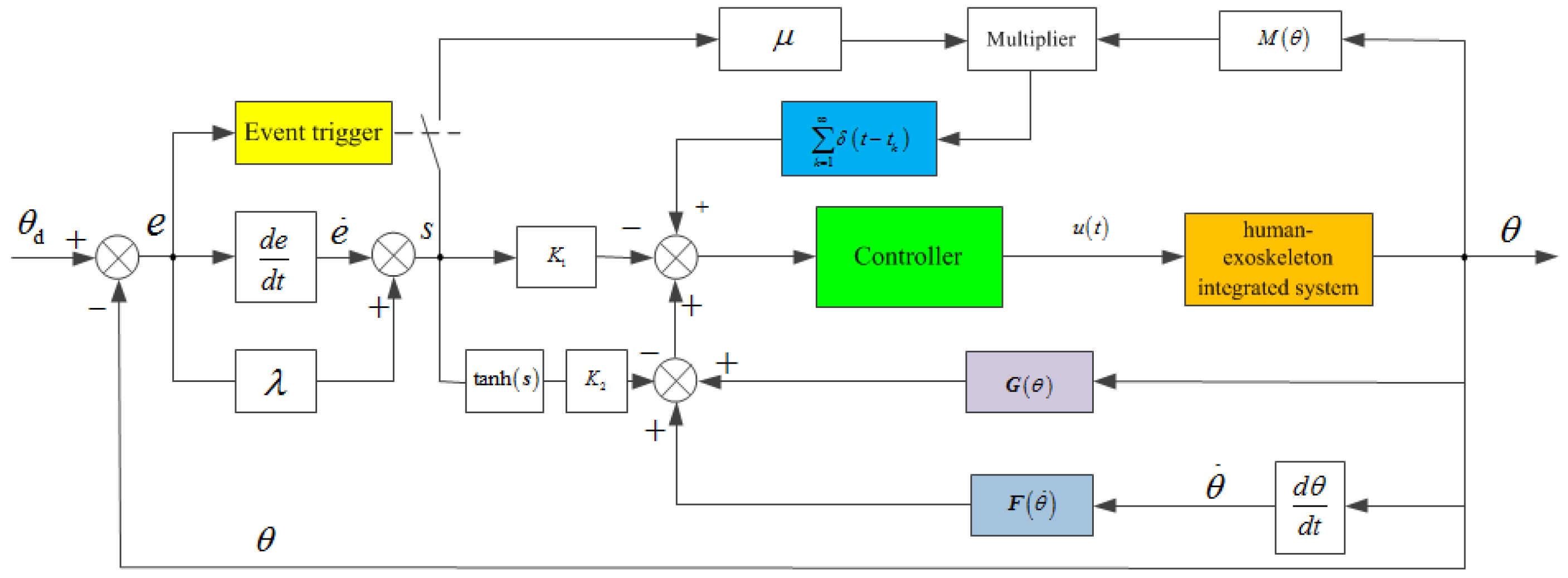
2.3. Event-Triggered Sliding Mode Impulsive Control

Let $e\left(t\right)={\theta }_d\left(t\right)-\theta \left(t\right)$ denote the tracking errors of trajectory. So $\dot{e}\left(t\right)={\dot{\theta }}_d\left(t\right)-\dot{\theta }\left(t\right)$, $\ddot{e}\left(t\right)={\ddot{\theta }}_d\left(t\right)-\ddot{\theta }\left(t\right)$. The feedback gain is $\Lambda =diag[\lambda ,\lambda ,\lambda ]\in {\mathbb{R}}^{3\times 3}$, and the reference angular velocity is defined as ${\dot{\theta }}_r\left(t\right)={\dot{\theta }}_d\left(t\right)+\Lambda e\left(t\right)$. So the reference angular acceleration is ${\ddot{\theta }}_r\left(t\right)={\ddot{\theta }}_d\left(t\right)+\Lambda \dot{e}\left(t\right)$. The sliding mode surface function is defined as follows:

$$s\left(t\right)=\dot{e}\left(t\right)+\Lambda e\left(t\right)={\dot{\theta }}_d\left(t\right)-\dot{\theta }\left(t\right)+\Lambda e\left(t\right)={\dot{\theta }}_{\mathrm{r}}\left(t\right)-\dot{\theta }\left(t\right)$$

(4)

Taking the derivative of the terms in the above formula, we get

$$\dot{s}\left(t\right)=\ddot{e}\left(t\right)+\Lambda \dot{e}\left(t\right)={\ddot{\theta }}_{\mathrm{d}}\left(t\right)-\ddot{\theta }\left(t\right)+\Lambda \dot{e}\left(t\right)={\ddot{\theta }}_{\mathrm{r}}\left(t\right)-\ddot{\theta }\left(t\right)$$

(5)

when a user is walking with the LLRER for gait rehabilitation, the gravity and Coulomb viscous friction always exist and can be identified and estimated in real-time by different methods [10]. So the online feedforward compensation control is adopted to counteract the gravity and friction, which always exist in LLRERs. To decrease the disturbances and system uncertainties and improve system robustness, a sliding mode control (SMC) method based on the exponential approach law is introduced. Furthermore, the hyperbolic tangent function is used to substitute the sign function for reducing chatter. It is worth noting that the external disturbance mainly comes from the ground shock force from the heel touching the ground to the toe leaving the ground and human–exoskeleton interaction force during the single leg swing. They are not continuous but discrete and impulsive. So, the Dirac delta function is used to imitate and against them, and event-triggered impulsive control (ETIC) is considered simultaneously [36,40,42]. So a feedback–feedforward hybrid controller with online gravity and friction compensation based on SMC and ETIC is designed as follows [36,40,51]:

$$u\left(t\right)=T+{\tau }_{\mathrm{d}}=G\left(\theta \left(t\right)\right)+F\left(\dot{\theta }\left(t\right)\right)-K_{1}s\left(t\right)-K_{2}tanh\left(s\left(t\right)\right)+\mu M\left(\theta \left(t\right)\right)s\left(t\right)\sum _{k=1}^{\infty }\delta \left(t-t_k\right)$$

(6)

where, $K_1,K_2\in {\mathbb{R}}_{\ge 0}$ are the parameters of SMC based on exponential approach law, and $\mu \in {\mathbb{R}}^{+}$ denotes the gain of impulsive controller.

Obviously, from (4), it is also a PD negative feedback control with feedback gain $\lambda$. The feedback compensation control system based on SMC and ETIC is depicted in Figure 2. According to (1), (4), (5), and (6), and letting $\Delta =M\left(\theta \right){\ddot{\theta }}_r+C(\theta ,\dot{\theta }){\dot{\theta }}_r$, the equation can be derived as follows:

$$M\left(\theta \right)\dot{s}\left(t\right)=\left(K_1{I}_3-C(\theta ,\dot{\theta })\right)s\left(t\right)+\Delta +K_2{I}_{3}tanh\left(s\left(t\right)\right)-\mu M\left(\theta \right)s\left(t\right)\sum _{k=1}^{\infty }\delta \left(t-t_k\right)$$

(7)

Because $M\left(\theta \right)$ is a symmetric positive-definite matrix, so $M^{-1}\left(\theta \right)$ exists. Therefore, (7) can be written as:

$$\dot{s}\left(t\right)=M^{-1}\left(\theta \right)\left[\left(K_1{I}_3-C(\theta ,\dot{\theta })\right)s\left(t\right)+\Delta +K_2{I}_{3}tanh\left(s\left(t\right)\right)\right]-\mu s\left(t\right)\sum _{k=1}^{\infty }\delta \left(t-t_k\right)$$

(8)

when $t\ne t_k$, $\delta (t-t_k)=0$, so (8) is simplified as

$$\dot{s}\left(t\right)=M^{-1}\left(\theta \right)\left[\left(K_1{I}_3-C(\theta ,\dot{\theta })\right)s\left(t\right)+\Delta +K_2{I}_{3}tanh\left(s\left(t\right)\right)\right]$$

(9)

In this paper, $s\left(t\right)$ is continuous except at the triggering instant $t=t_k$, so there exist ${lim}_{t\to t_k^{-}}s\left(t\right)=s\left(t_k^{-}\right)$ and ${lim}_{t\to t_k^{+}}s\left(t\right)=s\left(t_k^{+}\right)$. Generally, $s\left(t\right)$ is left continuous at $t_k$ for all k, thus $s\left(t_k^{-}\right)=s\left(t_k\right)$. By the property of Dirac function, ${\int }_{-\infty }^{+\infty }\delta \left(t-t_k\right)dt=1$ exists. So integrating both sides of system (8) from $t_k$ to $t_k^{+}$, one can obtain as follows: $\Delta s\left(t_k\right)=s\left(t_k^{+}\right)-s\left(t_k\right)=-\mu s\left(t_k\right)$. Thereby, $s\left(t_k^{+}\right)=(1-\mu )s\left(t_k\right)=(1-\mu )s\left(t_k^{-}\right)$. Consequently, combined with (9), the impulsive control system of the LLRER (1) under control law (6) can be described as:

$$\left\{\begin{array}{c}\dot{s}\left(t\right)=M^{-1}\left(\theta \right)\left[\left(K_1{I}_3-C(\theta ,\dot{\theta })\right)s\left(t\right)+\Delta +K_2{I}_{3}tanh\left(s\left(t\right)\right)\right],t\ne t_k,t\ge t_0,\hfill \\ s\left(t_k^{+}\right)=(1-\mu )s\left(t_k^{-}\right),t=t_k,k\in {\mathbb{Z}}^{+}.\hfill \end{array}\right.$$

(10)

 Remark 1.

In the control law (6), if $K_1=K_2=0$, and $\mu >0$, then (6) only includes ETIC with gravity and friction compensation as follows:

$$u\left(t\right)=T=G\left(\theta \right)+F\left(\dot{\theta }\right)-\mu M\left(\theta \right)s\left(t\right)\sum _{k=1}^{\infty }\delta \left(t-t_k\right)$$

(11)

Obviously, it is a special case of (6). At the instant $t\ne t_k$, $u\left(t\right)=T=G\left(\theta \right)+F\left(\dot{\theta }\right)$, the control law is irrelevant to state tracking errors, so there is no need to calculate and transmit errors. Only when $t=t_k$ should the desired human motion gait trajectories be received, and errors should be calculated and transferred. Therefore, compared to the time-triggered control method, (11) can greatly save computing resources and reduce the burden of the communication network.

 Remark 2.

In the control law (6), if $K_1>0$, $K_2=\mu =0$, then there is a proportional-derivative (PD) negative feedback control with gravity and friction compensation as in [11]. In this paper, the dynamic model contains Coulomb viscous friction, so it is more exact than in [11] and has better tracking performance.

 Remark 3.

In the control law (6), if $K_1>0$, $K_2>0$, $\mu =0$, then (6) is gravity and friction compensation control based on sliding mode control, which involved in [52].

 Remark 4.

In the control law (6), if $K_1>0$, $K_2=0$, $\mu >0$, then (6) consists of PD control and ETIC with gravity and friction compensation as in [36].

The triggering time sequence ${\{t_k,k\in {\mathbb{Z}}^{+}\}}_{k=1}^{\infty }$ in (7) is generated by the following impulsive event-triggered mechanism (IETM) [33,40]:

$$\left\{\begin{array}{c}{t}_k=min\left\{t_{k-1}+{\tau }_{max},t_k^{*}\right\}\hfill \\ t_k^{*}=inf\left\{t\ge t_{k-1}:V\left(s\left(t\right)\right)\ge e^{b-\eta \left(t-t_{k-1}\right)}V\left(s\left(t_{k-1}^{+}\right)\right)\right\}\hfill \end{array}\right.$$

(12)

where $t_{k-1}+{\tau }_{max}$ is called the forced triggering instant, $t_k^{*}$ is called the required event-triggered instant, b is a threshold parameter, $b>0$, $\eta$ is the exponential decay rate of the two consecutive triggered instants, and $\eta >0$. A Lyapunov function is chosen as $V\left(s\left(t\right)\right)=s^T\left(t\right)s\left(t\right)$, it depends on the state errors $s\left(t\right)$ at time t and the last time event-triggered instant $t_{k-1}$, respectively. $t_0\ge 0$ is a given initial instant and $s\left(t_0^{+}\right)$ is the initial state error of system at $t_0$. Note that the triggering time sequence ${\{t_k,k\in {\mathbb{Z}}^{+}\}}_{k=1}^{+\infty }$ may be different with the different choice of Lyapunov function $V\left(s\right(t\left)\right)$. The changes of b and $\eta$ will influence the triggering interval, and b may affect the boundary of $e^{b-\eta (t-t_{k-1})}V\left(s\left(t_{k-1}\right)\right)$. On the one hand, if b is larger, then the threshold is larger too. It means that there are larger triggering intervals but fewer triggering times. On the other hand, with a larger $\eta$, the threshold decays faster, the triggering intervals become smaller but the triggering times are greater.

 Remark 5.

When the exponential decay rate $\eta =0$, it is a special case of (12). Although it is easier, it is a constant unrelated to the triggering interval. So in practical application, one can adjust the two values of b and η simultaneously to obtain the desired system performance more easily.

 Remark 6.

In practical LLRER applications, the signals of the plantar pressure sensors and the human–exoskeleton interaction force sensors are used as the forced triggering conditions, and the Lyapunov function threshold of state error is used as the required event-triggered condition.

2.4. Definitions and Assumptions

The following definitions and assumptions are presented and exploited in the controller parameters design and stability analysis of the LLRER system.

 Definition 1.

For given $\alpha >0$ and any initial values of system (1), there exist a constant $T_0\in {\mathbb{R}}^{+}$, for $\forall t>T_0$, such that $e\left(t\right)\in {\mathsf{\Omega }}_s:=\left\{e\left(t\right)\in {\mathbb{R}}^n\parallel e\left(t\right)\parallel <\alpha \right\}$, where α is a boundary of the desired tracking error and $∥·∥$ is the Euclidean vector norm. So the LLRER system described by the Lagrangian dynamic model (1) is said to achieve practical tracking synchronization [36,53].

 Definition 2.

Let $N(t_0,t)$ denote the triggered times based on the event-triggered mechanism, so it holds

$$N\left(t_0,t\right)\ge \frac{t-t_0}{{\tau }_{max}}-1$$

(13)

where ${\tau }_{max}=max\{t_{k+1}-t_k\}$ is the maximum triggering interval, and ${\{t_k,k\in {\mathbb{Z}}^{+}\}}_{k=1}^{+\infty }$ is triggering time sequence generated by (12).

 Definition 3.

Given a locally Lipschitz function $V\left(x\right):{\mathbb{R}}^n\to {\mathbb{R}}^{+}$, the upper right–hand Dini derivative of $V\left(x\right)$ is defined as ${\mathrm{D}}^{+}V\left(x\right)={\overline{lim}}_{h\to 0^{+}}(V(x+h)-V\left(x\right))/h$.

 Assumption 1.

The hip joint (flexion/extension), knee joint (flexion/extension), and ankle joint (dorsiflexion/plantar flexion) are constrained to move only in the sagittal plane.

 Assumption 2.

We assume that $∥\dot{\theta }\left(t\right)∥$, $∥{\dot{\theta }}_d\left(t\right)∥$, and $∥{\ddot{\theta }}_d\left(t\right)∥$ are bounded, and there exist a positive constant $a_1\in {\mathbb{R}}^{+}$, such that $∥\dot{\theta }\left(t\right)∥\le a_1$.

According to above assumption, (5), and $\lambda >0$, hence, $∥{\ddot{\theta }}_r\left(t\right)∥$ are bounded, for $a_2\in {\mathbb{R}}^{+}$, it can be derived as follows:

$$\begin{array}{cc}\hfill ∥{\ddot{\theta }}_{\mathrm{r}}\left(t\right)∥& =∥{\ddot{\theta }}_{\mathrm{d}}\left(t\right)+\lambda \dot{e}\left(t\right)∥\hfill \\ \hfill & =∥{\ddot{\theta }}_{\mathrm{d}}\left(t\right)+\lambda \left({\dot{\theta }}_d\left(t\right)-\dot{\theta }\left(t\right)\right)∥\hfill \\ & \le ∥{\ddot{\theta }}_{\mathrm{d}}\left(t\right)∥+\lambda ∥{\dot{\theta }}_d\left(t\right)∥+\lambda \parallel \dot{\theta }\left(t\right)\parallel \hfill \\ \hfill & \le a_2\hfill \end{array}$$

(14)

 Remark 7.

All the dynamic parameters of the LLRER dynamic model (1) are identified as in [11,51]. In practical application, the joint angles, angular velocities, and angular accelerations are bounded. They can be accurately measured in real-time by encoders and inertial measurement units (IMU).

3. Main Results

3.1. Lyapunov Stability Analysis

 Theorem 1.

Given $K_1,K_2\in {\mathbb{R}}_{\ge 0}$ and the desired tracking error bound arbitrarily $\alpha >0$, if the impulsive control gain μ, feedback gain λ, and the maximum trigger interval ${\tau }_{max}$ satisfy the constraints as follows:

$$\left(i\right)0<\mu <1;\left(ii\right)\lambda >1;\left(iii\right){\tau }_{max}<-\frac{ln{(1-\mu )}^2}{\rho }$$

(15)

where $\beta =2\left(M_2{a}_2+k_c{a}_1\left(a_1+\alpha \right)+K_1\alpha +K_2\right)/M_1>0$, $\rho =\beta /\alpha >0$, then the asymptotic convergence of system (1) can be guaranteed. That means the LLRER system (1) can track the desired gait trajectory ${\theta }_d$ under the ETIC (7) and IETM (12) with the tracking error bound $\alpha$.

 Proof of Theorem 1 

There are three steps to prove Theorem 1, as follows.

• Step 1: Firstly, we should prove that, for given $\alpha >0$ and any initial values of system (1), there exists a constant $T_1\in {\mathbb{R}}^{+}$, if $\forall t>T_1$ satisfies, then it holds as follows:

  $$s\left(t\right)\in {\mathsf{\Psi }}_s:=\left\{s\left(t\right)\in {\mathbb{R}}^n\parallel s\left(t\right)\parallel <\alpha \right\}$$

  (16)
  To do this, a quadratic Lyapunov function $V\left(s\left(t\right)\right)=s^T\left(t\right)M\left(\theta \right)s\left(t\right)$ is constructed. If $s\left(t\right)\in {\mathbb{R}}^n/{\mathsf{\Psi }}_s$, due to (16), then $∥s\left(t\right)∥\ge \alpha$.
  On the one hand, when $t\in [t_k,t_{k+1})$, $t\ne t_k$, for above $V\left(s\right(t\left)\right)$, taking the Dini derivatives along the solutions of the first equation of (10), we get

  $$\begin{array}{cc}\hfill D^{+}V\left(s\left(t\right)\right)& =2s^{\mathrm{T}}\left(t\right)M\left(\theta \right)\dot{s}\left(t\right)+s^{\mathrm{T}}\left(t\right)\dot{M}\left(\theta \right)s\left(t\right)\hfill \\ \hfill & =2s^{\mathrm{T}}\left(t\right)\left(\Delta -C(\theta ,\dot{\theta })s\left(t\right)+K_{1}s\left(t\right)+K_{2}tanh\left(s\left(t\right)\right)\right)+s^{\mathrm{T}}\left(t\right)\dot{M}\left(\theta \right)s\left(t\right)\hfill \\ \hfill & =2s^{\mathrm{T}}\left(t\right)\left(\Delta +K_{1}s\left(t\right)+K_{2}tanh\left(s\left(t\right)\right)\right)+s^{\mathrm{T}}\left(t\right)(\dot{M}\left(\theta \right)-2C(\theta ,\dot{\theta }))s\left(t\right)\hfill \end{array}$$

  (17)
  By Property 1, i.e., (2), $s^{\mathrm{T}}\left(t\right)(\dot{M}\left(\theta \right)-2C(\theta ,\dot{\theta }))s\left(t\right)=0$. For $\Delta =M\left(\theta \right){\ddot{\theta }}_r\left(t\right)+C(\theta ,\dot{\theta }){\dot{\theta }}_r\left(t\right)$, thus

  $$\begin{array}{cc}\hfill D^{+}V\left(s\left(t\right)\right)& =2s^{\mathrm{T}}\left(t\right)\left(\Delta +K_{1}s\left(t\right)+K_{2}tanh\left(s\left(t\right)\right)\right)\le 2∥s^{\mathrm{T}}\left(t\right)∥\left(\parallel \Delta \parallel +K_1\parallel s\left(t\right)\parallel +K_2\right)\hfill \\ \hfill & =2∥s^{\mathrm{T}}\left(t\right)∥\left(\parallel M\left(\theta \right)\parallel ∥{\ddot{\theta }}_{\mathrm{r}}\left(t\right)∥+\parallel C(\theta ,\dot{\theta })\parallel ∥{\dot{\theta }}_{\mathrm{r}}\left(t\right)∥+K_1\parallel s\left(t\right)\parallel +K_2\right)\hfill \end{array}$$

  (18)
  By Property 2, i.e., (3), we have $\parallel M\left(\theta \right)\parallel \le M_2$, $\parallel C(\theta ,\dot{\theta })\parallel \le k_c\parallel \dot{\theta }\left(t\right)\parallel$. According to Assumption 2, (14), and (4), we have $\parallel \dot{\theta }\left(t\right)\parallel \le a_1$, $\parallel {\ddot{\theta }}_r\left(t\right)\parallel \le a_2$, and $∥{\dot{\mathit{\theta }}}_{\mathrm{r}}\left(t\right)∥=\parallel \dot{\mathit{\theta }}\left(t\right)+\mathit{s}\left(t\right)\parallel \le \parallel \dot{\mathit{\theta }}\left(t\right)\parallel +\parallel \mathit{s}\left(t\right)\parallel \le a_1+\parallel s\left(t\right)\parallel$. Accordingly, it can be derived as

  $$D^{+}V\left(s\left(t\right)\right)\le 2∥s^{\mathrm{T}}\left(t\right)∥\left(M_2{a}_2+k_c{a}_1\left(a_1+\parallel s\left(t\right)\parallel \right)+K_1\parallel s\left(t\right)\parallel +K_2\right)$$

  (19)
  Since $\parallel s\left(t\right)\parallel \ge \alpha$, hence, from this one can get that

  $$D^{+}V\left(s\left(t\right)\right)\le 2∥s^{\mathrm{T}}\left(t\right)∥\parallel s\left(t\right)\parallel \left(M_2{a}_2+k_c{a}_1\left(a_1+\alpha \right)+K_1\alpha +K_2\right)/\alpha$$

  (20)
  Due to (3), there exists $M_1\le \parallel M\left(\theta \right)\parallel$, hence, (20) can be written as

  $$\begin{array}{cc}\hfill & D^{+}V\left(s\left(t\right)\right)\le 2\left(M_2{a}_2+k_c{a}_1\left(a_1+\alpha \right)+K_1\alpha +K_2\right)∥s^{\mathrm{T}}\left(t\right)∥\parallel M\left(\theta \right)\parallel \parallel s\left(t\right)\parallel /\left(\alpha M_1\right)\hfill \\ \hfill & =2\left(M_2{a}_2+k_c{a}_1\left(a_1+\alpha \right)+K_1\alpha +K_2\right)∥s^{\mathrm{T}}\left(t\right)M^{\frac{T}{2}}\left(\theta \right)∥∥M^{\frac{1}{2}}\left(\theta \right)s\left(t\right)∥/\left(\alpha M_1\right)\hfill \\ \hfill & =2\left(M_2{a}_2+k_c{a}_1\left(a_1+\alpha \right)+K_1\alpha +K_2\right)s^{\mathrm{T}}\left(t\right)M\left(\theta \right)s\left(t\right)/\left(\alpha M_1\right)\hfill \\ \hfill & =(\beta /\alpha )V\left(s\right(t\left)\right)=\rho V\left(s\right(t\left)\right)\hfill \end{array}$$

  (21)
  Because $s\left(t\right)$ is left continuous at $t_k$, so $t\left(t_{k-1}^{+}\right)=s\left(t_k^{-}\right)=s\left(t_k\right)$. We integrate both sides of the above inequality (21) from $t_{k-1}$ to t, and get that

  $$ln\frac{V\left(s\right(t\left)\right)}{V\left(s\left(t_{k-1}^{+}\right)\right)}\le \rho \left(t-t_{k-1}\right)$$

  (22)

  from which one can obtain

  $$V\left(s\left(t\right)\right)\le V\left(s\left(t_{k-1}^{+}\right)\right)e^{\rho \left(t-t_{k-1}\right)},t\in \left[t_k,t_{k+1}\right),k=1,2,3\dots$$

  (23)
  On the other hand, at the impulsive instant, when $t=t_k$, $V\left(s\right(t\left)\right)$ is expressed as $V\left(s\left(t_k^{+}\right)\right)=s^T\left(t_k^{+}\right)M\left(\theta \right)s\left(t_k^{+}\right)$. We substitute the second equation of the impulsive system (10) into the above equality to get

  $$\begin{array}{cc}\hfill V\left(s\left(t_k^{+}\right)\right)& =(1-\mu )s^{\mathrm{T}}\left(t_k^{-}\right)M\left(\theta \right)(1-\mu )s\left(t_k^{-}\right)\hfill \\ \hfill & ={(1-\mu )}^2{s}^{\mathrm{T}}\left(t_k^{-}\right)M\left(\theta \right)s\left(t_k^{-}\right)={(1-\mu )}^{2}V\left(s\left(t_k^{-}\right)\right)\hfill \end{array}$$

  (24)
  By the constraint $\left(i\right)$$0<\mu <1$, we have ${(1-\mu )}^2<1$. It implies that the Lyapunov function decreases gradually.

• Step 2: Next, we will prove that, for $t\in [t_k,t_{k+1})$, $k=1,2,3\cdots$, the inequality holds as follows:

  $$V\left(s\left(t\right)\right)\le {(1-\mu )}^{2(k-1)}V\left(s\left(t_0^{+}\right)\right)e^{\rho \left(t-t_0\right)}$$

  (25)
  (a). If $k=1$, then $t\in [t_0,t_1)$. From inequalities (23) and (24), one can obtain

  $$V\left(s\left(t\right)\right)\le V\left(s\left(t_0^{+}\right)\right)e^{\rho \left(t-t_0\right)}={(1-\mu )}^{2\times (1-1)}V\left(s\left(t_0^{+}\right)\right)e^{\rho \left(t-t_0\right)}$$

  (26)

  which means (25) holds.
  (b). If $k=2$, then $t\in [t_1,t_2)$. From inequalities (23) and (24), one has

  $$\begin{array}{cc}\hfill V\left(s\right(t\left)\right)& \le V\left(s\left(t_1^{+}\right)\right)e^{\rho \left(t-t_1\right)}={(1-\mu )}^{2}V\left(s\left(t_1^{-}\right)\right)e^{\rho \left(t-t_1\right)}\hfill \\ \hfill & ={(1-\mu )}^{2}V\left(s\left(t_0^{+}\right)\right)e^{\rho \left(t_1-t_0\right)}{e}^{\rho \left(t-t_1\right)}\hfill \\ \hfill & ={(1-\mu )}^{2\times (2-1)}V\left(s\left(t_0^{+}\right)\right)e^{\rho \left(t-t_0\right)}\hfill \end{array}$$

  (27)

  which means (25) also holds.
  (c). Assume that when $k=n\ge 3$, $t\in [t_{n-1},t_n)$, the inequality (25) holds as follows:

  $$V\left(s\left(t\right)\right)\ge {(1-\mu )}^{2\times (n-1)}V\left(s\left(t_0^{+}\right)\right)e^{\rho \left(t-t_0\right)}$$

  (28)
  Thereby, when $k=n+1$, $t\in [t_n,t_{n+1})$, from inequality (23) and (24), we can conclude that

  $$\begin{array}{cc}\hfill V\left(s\right(t\left)\right)& \le V\left(s\left(t_n^{+}\right)\right)e^{\rho \left(t-t_n\right)}={(1-\mu )}^{2}V\left(s\left(t_n^{-}\right)\right)e^{\rho \left(t-t_n\right)}\hfill \\ \hfill & \le {(1-\mu )}^2{(1-\mu )}^{2\times (n-1)}V\left(s\left(t_0^{+}\right)\right)e^{\rho \left(t_n-t_0\right)}{e}^{\rho \left(t-t_n\right)}\hfill \\ \hfill & ={(1-\mu )}^{2n}V\left(s\left(t_0^{+}\right)\right)e^{\rho \left(t-t_0\right)}\hfill \end{array}$$

  (29)
  That means when $k=n+1$, inequality (25) also holds. Therefore, synthesizing (a), (b), and (c) by the method of mathematical induction, when $t\in [t_{k-1},t_k)$, $k\in {\mathbb{Z}}^{+}$, inequality (25) always holds.
  Due to $0<{(1-\mu )}^2<1$, from (13) and (25), one has

  $$\begin{array}{cc}\hfill V\left(s\right(t\left)\right)& \le {(1-\mu )}^{2\left(\frac{\left(t-t_0\right)}{{\tau }_{max}}-1\right)}V\left(s\left(t_0^{+}\right)\right)e^{\rho \left(t-t_0\right)}\hfill \\ \hfill & ={(1-\mu )}^{-2}V\left(s\left(t_0^{+}\right)\right)e^{\left(\frac{ln{(1-u)}^2}{{\tau }_{max}}+\rho \right)\left(t-t_0\right)}\hfill \end{array}$$

  (30)

  from constraint $\left(ii\right)$, we have $\frac{ln{(1-u)}^2}{{\tau }_{max}}+\rho <0$. Hence, when $k\to +\infty$, there exists $V\left(s\right(t\left)\right)\to 0$ as $t\to +\infty$, which means that $V\left(s\right(t\left)\right)$ is monotonically decreasing to $s\left(t\right)\in {\mathsf{\Omega }}_s$, and the system (1) under control law (6) is exponential asymptotic stable. In another words, there always exists $T_1>0$, such that $\parallel s\left(t\right)\parallel \le \alpha$ for $\forall t>T_1$.

• Step 3: Finally, we will prove that, there exists $T_0>T_1$ such that $\parallel e\left(t\right)\parallel <\alpha$ for $\forall t>T_0$. If $e\left(t\right)\in {\mathbb{R}}^n/{\mathsf{\Omega }}_s$, then $\parallel e\left(t\right)\parallel \ge \alpha$ holds, Owing to $\parallel s\left(t\right)\parallel \le \alpha$, so $\parallel s\left(t\right)\parallel \le \parallel e\left(t\right)\parallel$. We multiply both sides of the above inequality by $\parallel e^T\left(t\right)\parallel$ to get

  $$\parallel e^T\left(t\right)\parallel \parallel s\left(t\right)\parallel \le {\parallel e\left(t\right)\parallel }^2=e^T\left(t\right)e\left(t\right)$$

  (31)
  We choose a quadratic Lyapunov function: $V(\theta ,\dot{\theta },t)=\frac{1}{2}{e}^T\left(t\right)e\left(t\right)$. From (4) and (31), we can derive

  $$\begin{array}{cc}\hfill \dot{V}(\theta ,\dot{\theta },t)& =\frac{1}{2}\left({\dot{e}}^{\mathrm{T}}\left(t\right)e\left(t\right)+e^{\mathrm{T}}\left(t\right)\dot{e}\left(t\right)\right)\hfill \\ \hfill & =-\lambda e^{\mathrm{T}}\left(t\right)e\left(t\right)+\frac{1}{2}\left(s^{\mathrm{T}}\left(t\right)e\left(t\right)+e^{\mathrm{T}}\left(t\right)s\left(t\right)\right)\hfill \\ \hfill & \le -\lambda e^{\mathrm{T}}\left(t\right)e\left(t\right)+∥e^{\mathrm{T}}\left(t\right)∥\parallel s\left(t\right)\parallel \hfill \\ \hfill & \le -\lambda e^{\mathrm{T}}\left(t\right)e\left(t\right)+e^{\mathrm{T}}\left(t\right)e\left(t\right)\hfill \\ \hfill & =(1-\lambda )e^{\mathrm{T}}\left(t\right)e\left(t\right)\hfill \end{array}$$

  (32)
  According to the constraint $\left(iii\right)$$\lambda >1$, we have $\dot{V}(\theta ,\dot{\theta },t)<0$, and it is negative definite function when $e\left(t\right)\in {\mathbb{R}}^n/{\mathsf{\Omega }}_s$. Therefore, the Lyapunov function is gradually decreased until $e\left(t\right)\in {\Omega }_s$. According to definition 1, there always exist $T_0>T_1$, for $\forall t>T_0$, $\parallel e\left(t\right)\parallel <\alpha$ holds. It means that the practical tracking synchronization is within a desired tracking error bound $\alpha$ and the tracking errors $e\left(t\right)$ remain within the desired finite ball ${\mathsf{\Omega }}_s$. The proof of Theorem 1 is completed.

□

 Remark 8.

In Theorem 1, the constraints are sufficient and non-essential conditions. It implies that if the conditions are not met, the joint angles of the LLRER system may be able to track the desired gait trajectory.

As in Remark 1, if the control law only includes ETIC with gravity and friction compensation as (11), i.e., $K_1=K_2=0$, $\mu \ne 0$, we substitute it to (15) in Theorem 1, then one can obtain as follows:

 Corollary 1.

Given the desired tracking error bound arbitrarily $\alpha >0$, if the impulsive control gain μ, feedback gain λ, and the maximum trigger interval ${\tau }_{max}$ satisfy the constraints as follows:

$$\left(i\right)0<\mu <1;\left(ii\right)\lambda >1;\left(iii\right){\tau }_{max}<-\frac{ln{(1-\mu )}^2}{\rho }$$

(33)

where $\beta =2\left(M_2{a}_2+k_c{a}_1\left(a_1+\alpha \right)\right)/M_1>0$, $\rho =\beta /\alpha >0$, then the asymptotic convergence of system (1) can be guaranteed. That means the LLRER system (1) can track the desired gait trajectory ${\theta }_d$ under the ETIC (11) and IETM (12) with the tracking error bound α.

As in Remark 4, if the control law consists of PD control and ETIC with gravity and friction compensation, i.e., $K_1>0$, $K_2=0$, $\mu >0$, and we substitute it into (15) in Theorem 1, then one can obtain as follows:

 Corollary 2.

Given the desired tracking error bound arbitrarily $\alpha >0$, if the impulsive control gain μ, feedback gain λ, and the maximum trigger interval ${\tau }_{max}$ satisfy the constraints as follows:

$$\left(i\right)0<\mu <1;\left(ii\right)\lambda >1;\left(iii\right){\tau }_{max}<-\frac{ln{(1-\mu )}^2}{\rho }$$

(34)

where $\beta =2\left(M_2{a}_2+k_c{a}_1\left(a_1+\alpha \right)+K_1\alpha \right)/M_1>0$, $\rho =\beta /\alpha >0$, then the asymptotic convergence of system (1) can be guaranteed. That means the LLRER system (1) can track the desired gait trajectory ${\theta }_d$ under the ETIC (11) and IETM (12) with the tracking error bound α.

3.2. Exclusion of Zeno Behavior

 Theorem 2.

There is no Zeno behavior for system (10) under IETM (12) if the triggering parameters satisfy the constraints as follows:

$$b>0,\eta >0,\eta +\rho >0$$

(35)

 Proof of Theorem 2 

We consider three cases.

• Case (a): Triggering time sequence ${\{t_k,k\in {\mathbb{Z}}^{+}\}}_{k=1}^{+\infty }$ entirely consists of the forced triggering instants ${\{t_{k-1}+{\tau }_{max}\}}_{k=1}^{+\infty }$. In this case, it follows the assumption $t_k-t_{k-1}={\tau }_{max}>0$, which means with certainty that the Zeno behavior is excluded.

• Case (b): Triggering time sequence ${\{t_k,k\in {\mathbb{Z}}^{+}\}}_{k=1}^{+\infty }$ fully consists of the required event-triggered instants ${\left\{t_k^{*}\right\}}_{k=1}^{+\infty }$. In this case, according to (12) and (23), it holds that

  $$e^{b-\eta \left(t_k-t_{k-1}\right)}V\left(s\left(t_{k-1}^{+}\right)\right)\le V\left(s\left(t_k\right)\right)\le e^{\rho \left(t_k-t_{k-1}\right)}V\left(s\left(t_{k-1}^{+}\right)\right)$$

  (36)
  Due to $V\left(s\left(t_{k-1}^{+}\right)\right)\ge 0$, hence, $e^{b-\eta \left(t_k-t_{k-1}\right)}\le e^{\rho \left(t_k-t_{k-1}\right)}$. For $\rho >0$, $\eta >0$, thus yielding $b-\eta \left(t_k-t_{k-1}\right)\le \rho \left(t_k-t_{k-1}\right)$. It can be deduced that $t_k-t_{k-1}\ge b/(\eta +\rho )>0$. Repeating this procedure for $t\in [t_{k-1},t_k)$, $k=1,2,3\cdots ,+\infty$, we obtain $t_k-t_0\ge bk/(\eta +\rho )$. If the constraints satisfy $b>0$, $\eta >0$, $\eta +\rho >0$, then $t_k\ge \frac{bk}{\eta +\rho }+t_0\to +\infty$ as $k\to +\infty$. This implies that the Zeno behavior is excluded.

• Case (c): Triggering time sequence ${\{t_k,k\in {\mathbb{Z}}^{+}\}}_{k=1}^{+\infty }$ consists of both event-triggered instants and forced triggering instants. In this case, we assume instant Q is the Zeno instant, so $Q\ne +\infty$. Let $P=(Q-{\tau }_{max}/\xi )\vee t_0$, where $\xi >1$ and $Q-{\tau }_{max}<P$, so the interval $[P,Q)$ consists of infinitely many impulsive instants. If there exists a forced triggering instant in $[P,Q)$, then we claim that there must be only one forced triggering instant called $\overline{t}$. Otherwise, it will contradict the definition of P. Obviously, all $t_k\in (\overline{t},Q)$ are required event-triggered instants. From case (b), it holds $t_k\to +\infty$ as $k\to +\infty$, which contradicts the definition of instant Q. Inversely, if there is no forced triggering instant in $[P,Q)$, then the Zeno behavior can also be excluded [33,54].

In summary, in the above three cases, it can be obtained that if constraints (35) are satisfied, then the triggering interval exists definitely, which implies that the Zeno behavior of system (10) under IETM (12) is excluded. So far the proof of Theorem 2 is completed.

□

As in Remark 5, if $\eta =0$, we substitute it to (35) in Theorem 2, then one can obtain:

 Corollary 3.

There is no Zeno behavior for system (10) under IETM (12) if the triggering parameters satisfy constraints: $b>0$, $\rho >0$ [55].

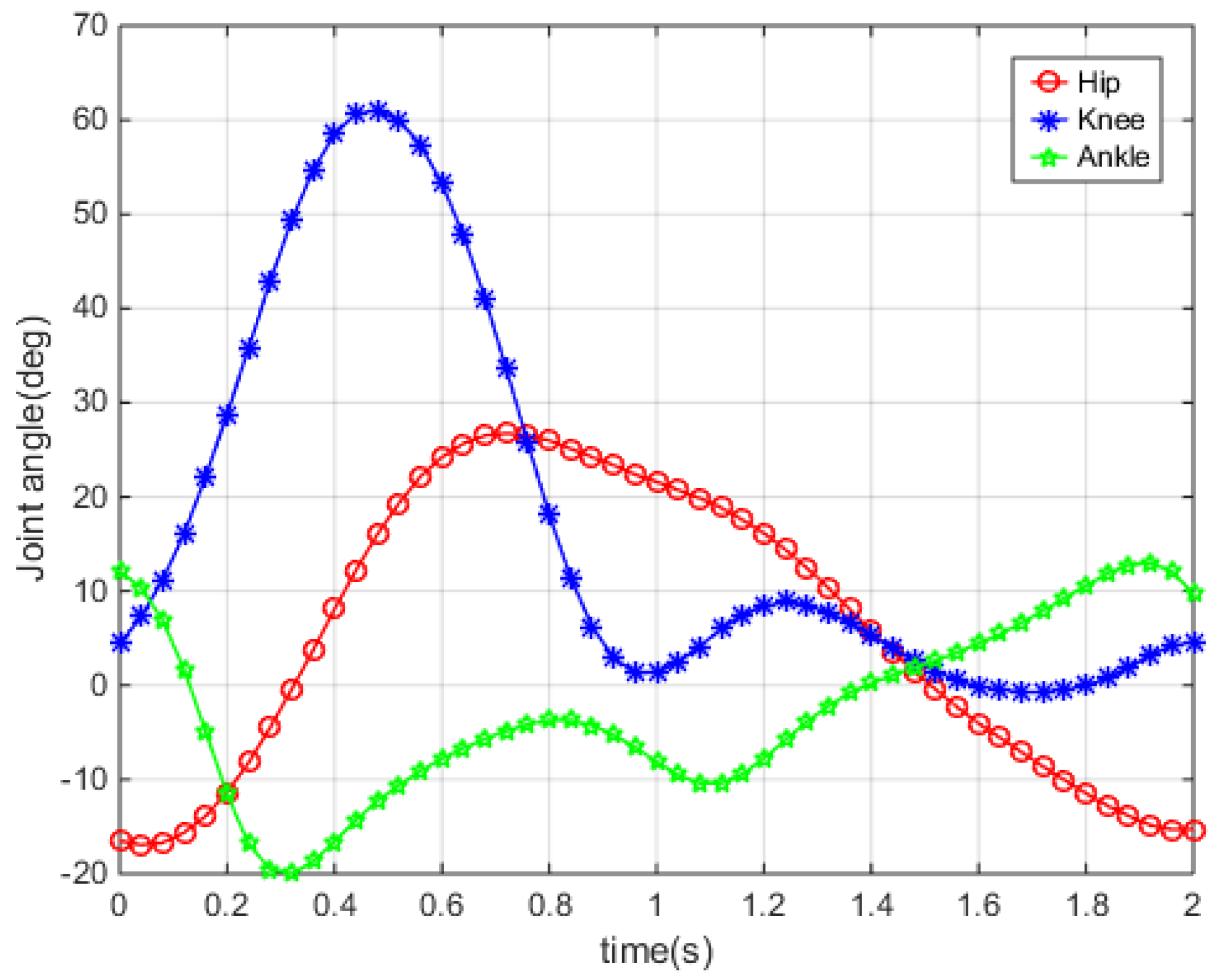
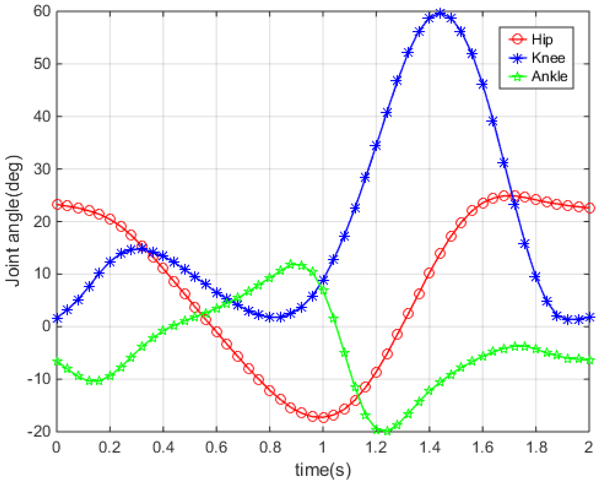
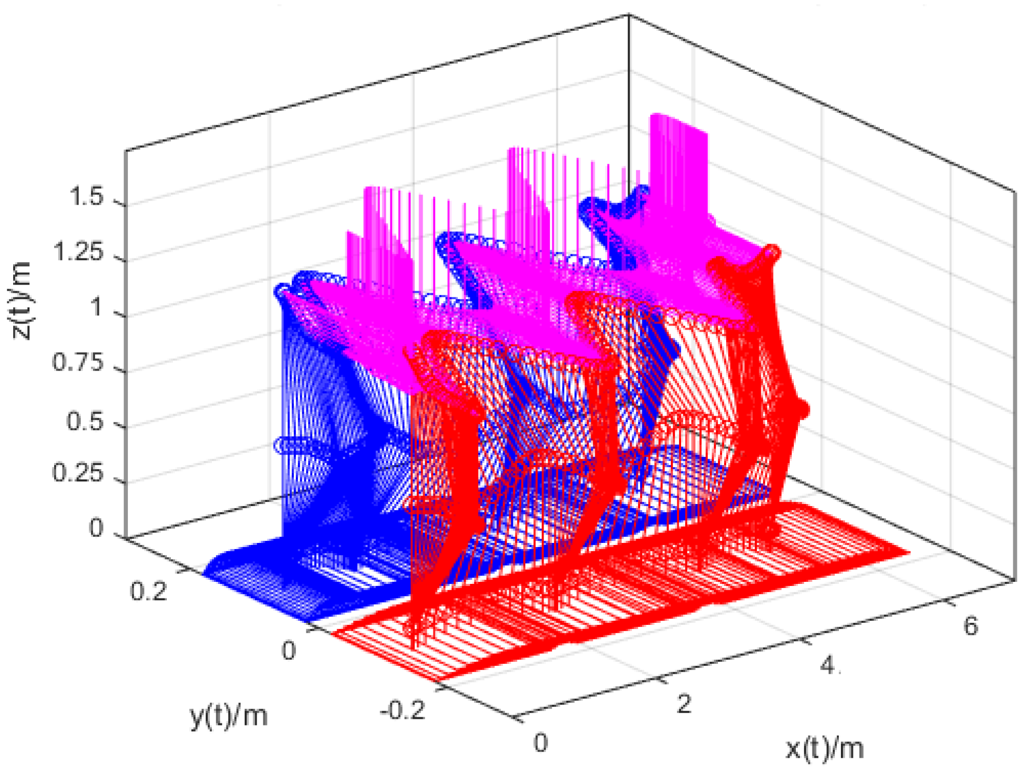
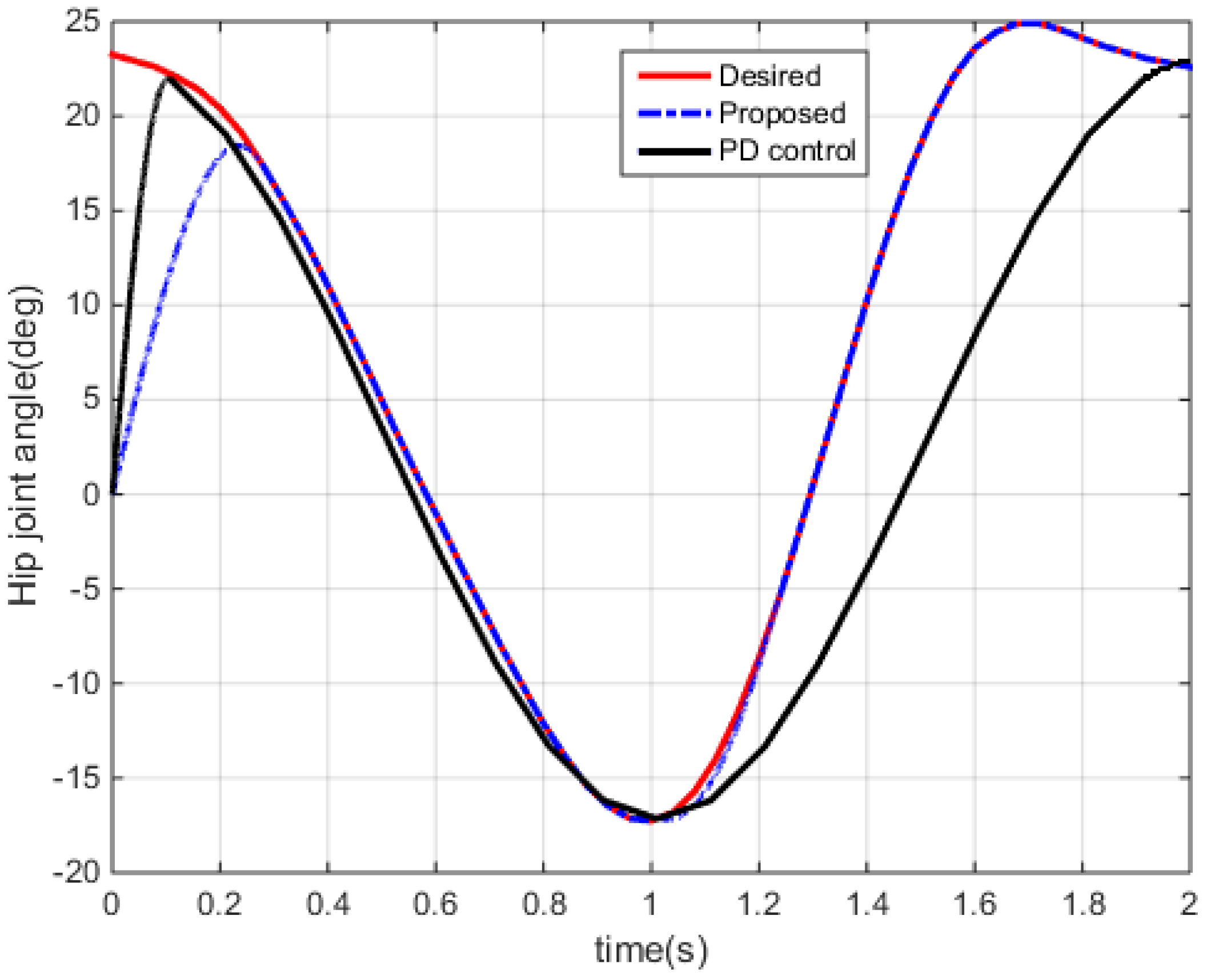
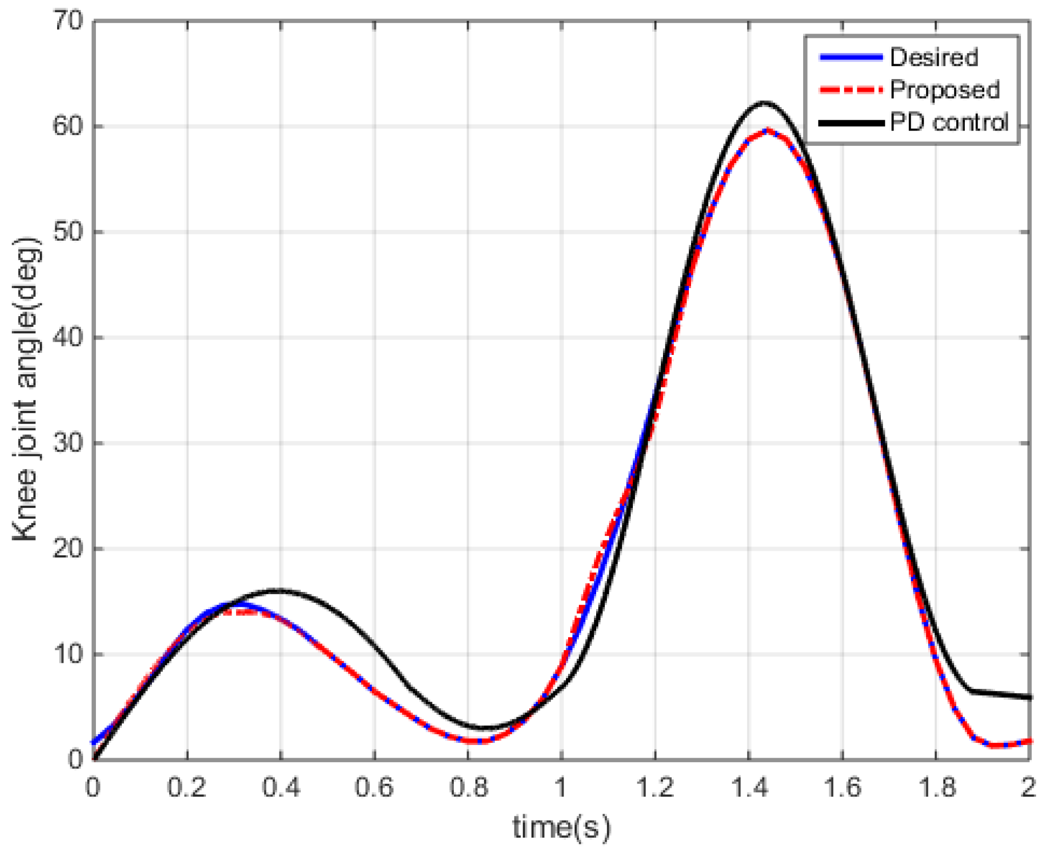
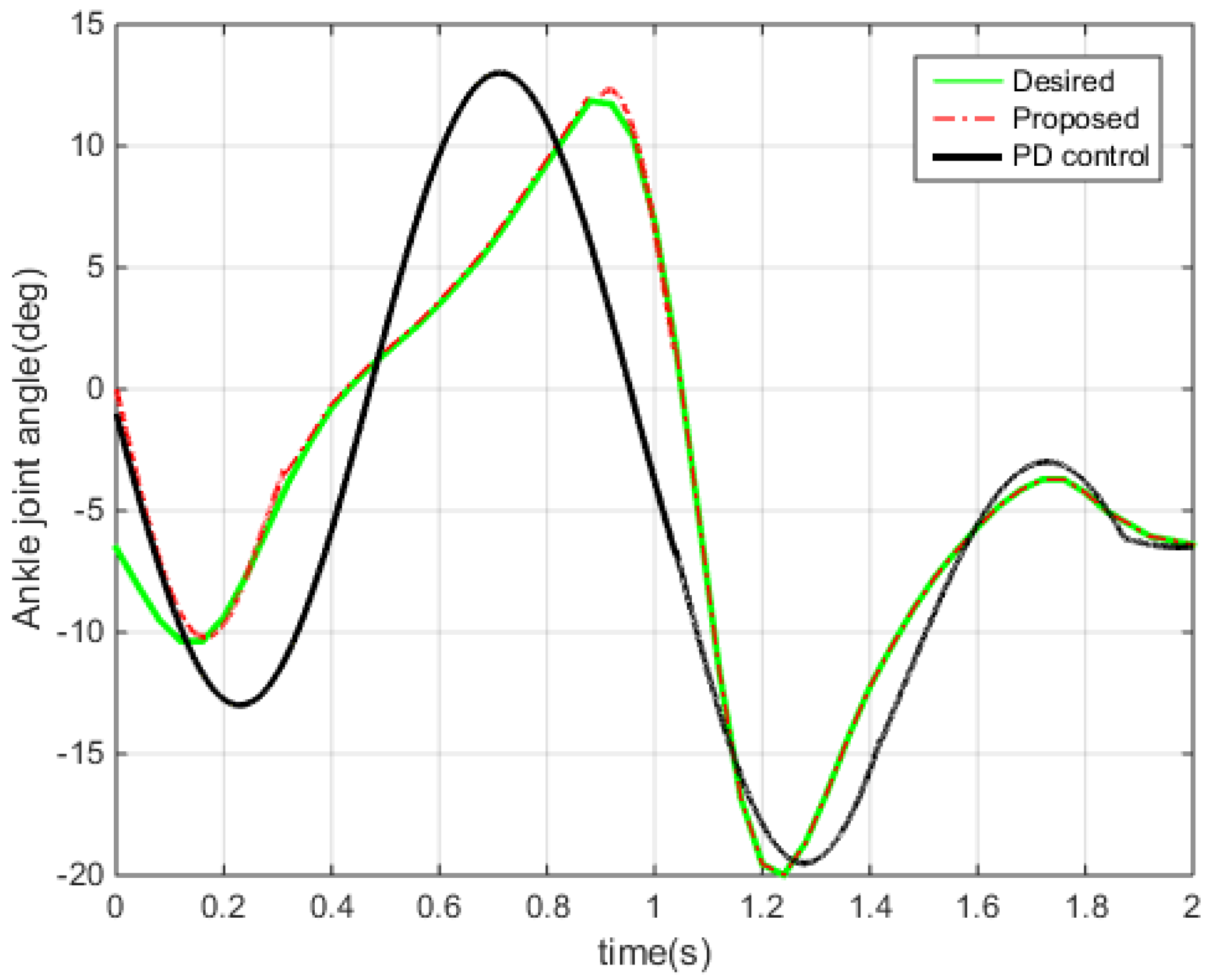
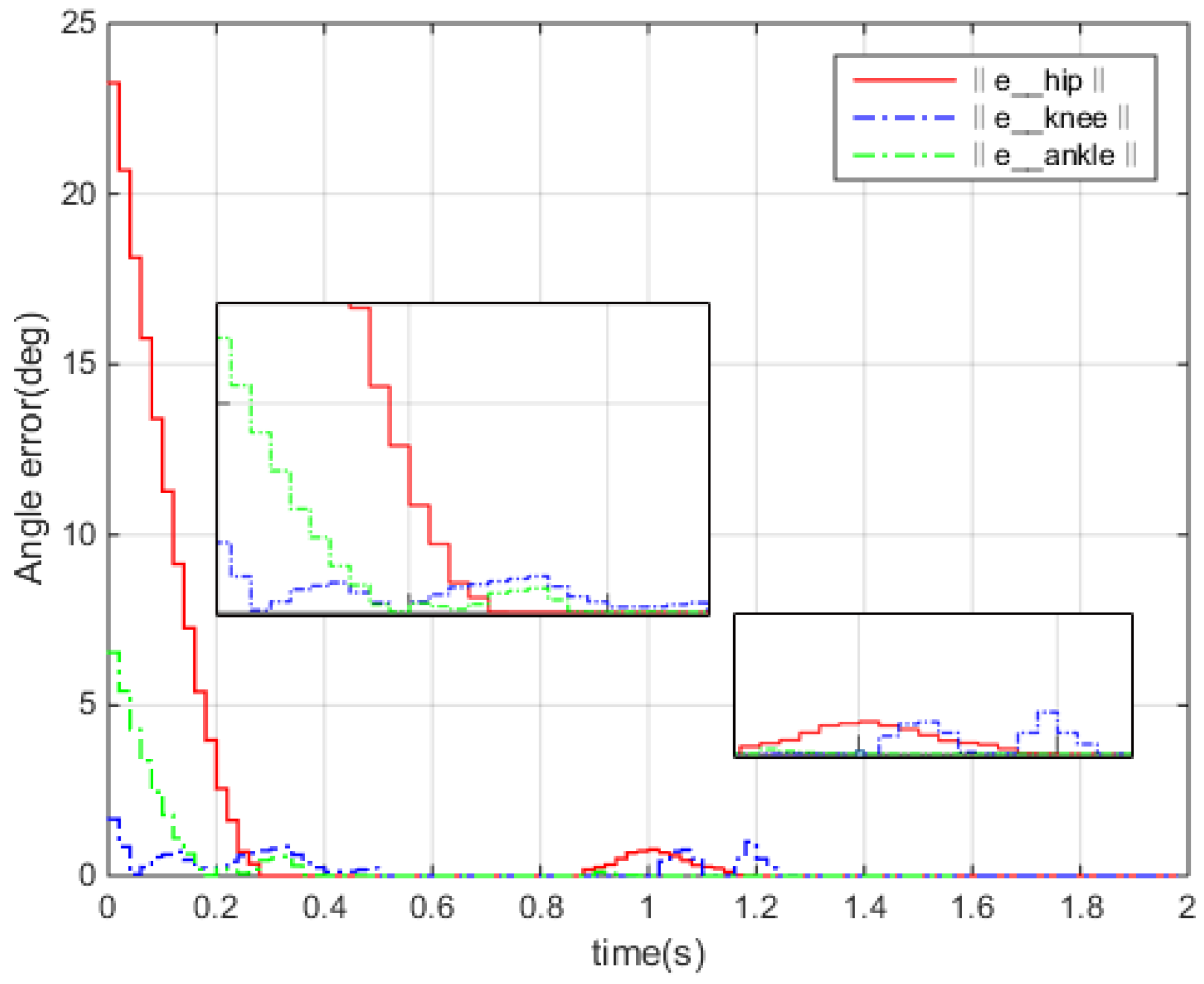
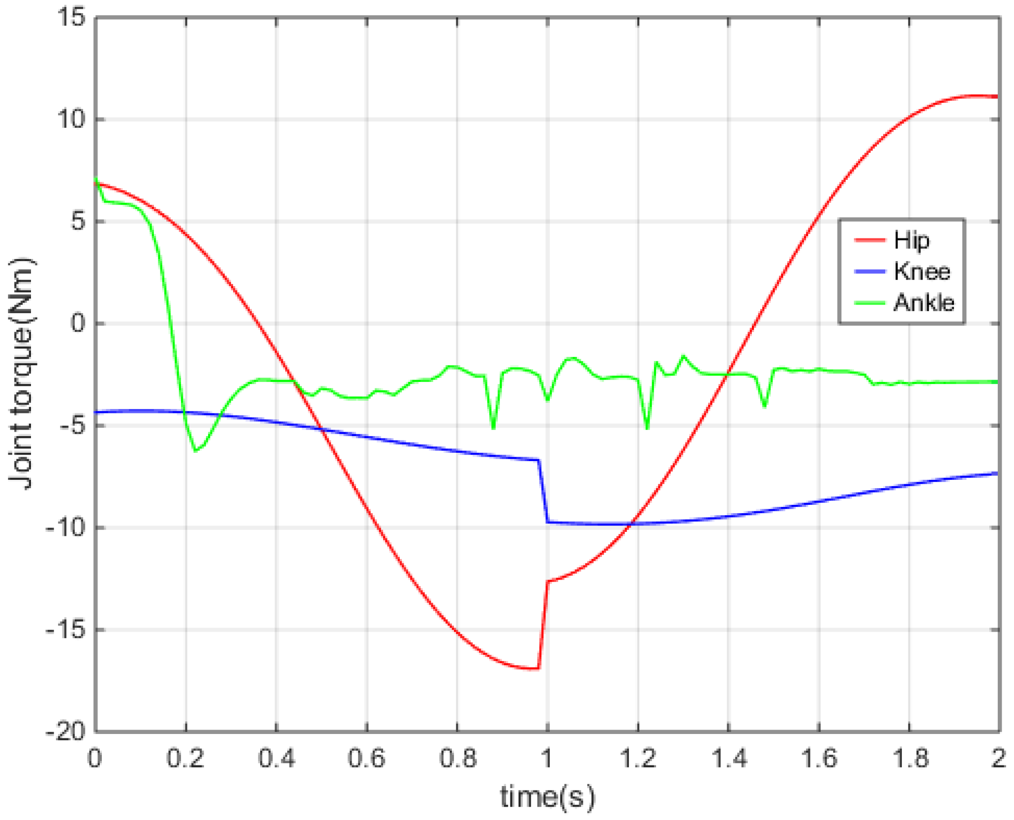
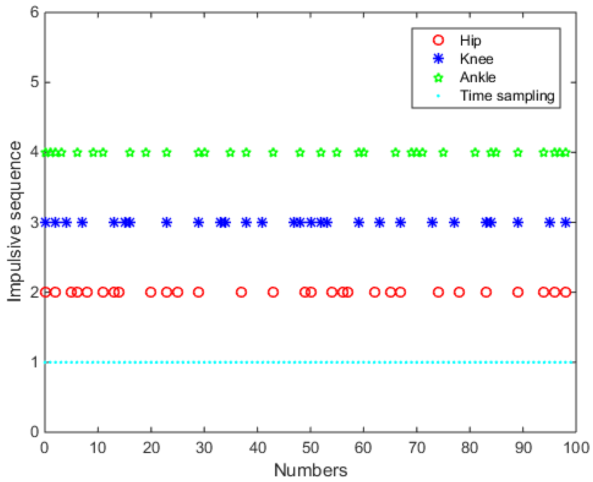
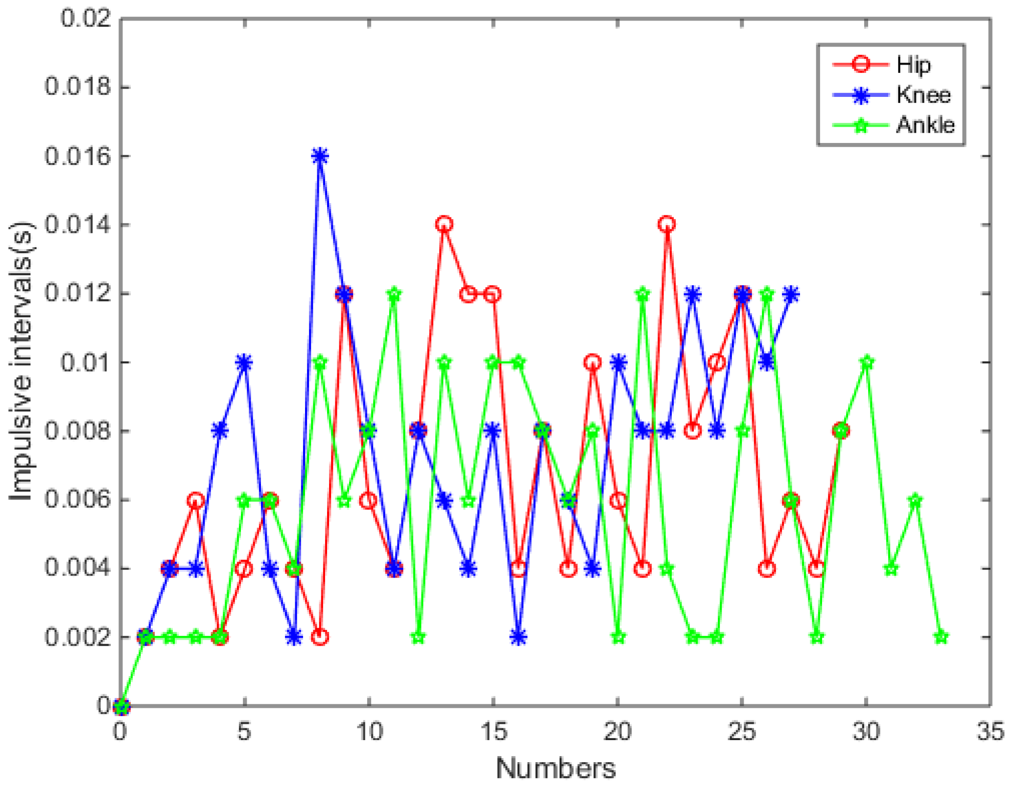
4. Numerical Simulation

To verify the effectiveness of the proposed control strategy, a simulation study of human motion gait tracking for the CUHK-EXO LLRER human–exoskeleton integrated system is carried out in MATLAB. The user’s height is 170 cm, the weight is 65 kg, and the mass of the CUHK-EXO LLRER is 20 kg. By measurement, estimation, and dynamic parameter identification, one can obtain these parameters and the dynamic model as in [10,47,48]: $m_1=9.6$ kg, $m_2=5.3$ kg, $m_3=1.4$ kg, $L_1=0.46$ m, $L_2=0.4$ m, $L_3=0.28$ m, $f_{v1}=0.062$, $f_{c1}=-1.731$, $f_{v2}=0.031$, $f_{c2}=-0.012$, $f_{v3}=0.157$, and $f_{c3}=-0.632$. According to the reference [36], we set several basic parameters as follows: $M_1=2.36$, $M_2=9.2$, $k_c=0.65$, $\alpha =0.02$, $a_1=1.52$, $a_2=0.03$, $\mu =0.98$, $\lambda =10$, $K_1=12$, and $K_2=1.4$; then we substitute them into Theorem 1 and Theorem 2 to get the values range of ${\tau }_{max}$, b, and $\eta$; at last we take a group of parameters with good tracking performance as the final parameters of the controller: ${\tau }_{max}=0.0152$, $b=1.34$, and $\eta =0.68$. Generally, a healthy human body always has a symmetrical gait, and the motion trajectories of the two legs are exactly the same except for half a gait cycle ahead or behind. When a healthy human walks, the angles of the hip, knee, and ankle joints of the lower limb can be used as the desired trajectories for patients with lower limb movement disorders at the early stage of passive rehabilitation training. As shown in Figure 3 and Figure 4, they are common gait trajectories obtained from CGA (Clinical Gait Analysis) and CASIA (Chinese Academy of Sciences Institute of Automation) Gait Dataset B [6,47,56]. We take the three-link simplified structure of the CUHK-EXO human–exoskeleton integrated system as the dynamic model to carry out gait tracking simulation. We obtain the 3D simulation diagram of walking gait, as shown in Figure 5. In the simulation, the step distance is 2 m, the gait cycle is 2 s, and the walking velocity of the human–exoskeleton integrated system is 1 m/s. It walks three gait periods and goes forward 6 m in 6 s. In a gait cycle, there are 100 time-sampling points, and the sampling interval is 2 ms. Based on the dynamic model of CUHK-EXO human exoskeleton integrated system, with the desired trajectory input as in Figure 4, the gait tracking results are shown in Figure 6, Figure 7 and Figure 8 for the proposed hybrid control strategy in this paper and the PD control method with gravity and friction compensation [54,55]. In the simulation, the hip joint and knee joint are disturbed by the human–exoskeleton interaction forces, the disturbances are simulated by the sine wave signal, ${\tau }_{d1}={\tau }_{d2}=0.3sin\left(t\right)$, and the ankle joint is disturbed mainly by the shock force from the ground, the disturbance is simulated by the square wave signal, ${\tau }_{d3}=1.5square(2\ast pi\ast t,10)$. At the beginning of human motion, the system is in the initial state, the human–exoskeleton stands on both legs, all the angles of the joints are zeros, $\left[{\theta }_1\left(0\right){\theta }_2\left(0\right){\theta }_3\left(0\right)\right]=[0°0°0°]$, but the desired angles of joint are $\left[{\theta }_{1d}\left(0\right){\theta }_{2d}\left(0\right){\theta }_{3d}\left(0\right)\right]=[23°1°-1°]$. When the system starts, for existing large tracking errors, the output torques of joint actuators increase rapidly, and the hip joint angle achieves real-time gait tracking with bounded errors only in 0.24 s; the other two joints take 0.35 s and 0.37 s, respectively. As shown in Figure 6, Figure 7 and Figure 8, the hybrid control strategy proposed in this paper can achieve complete tracking with bounded error after the control system runs for 0.3 s. As shown in Figure 9, the maximum tracking error angles of the hip, knee, and ankle joints are only 1°, 1.2°, and 1.5° when the system runs stably, and the maximum error rates of gait tracking are 4%, 2%, and 7.5%, respectively. It shows that the control system has a fast response speed and small tracking error. So it can achieve perfect gait tracking. However, compared to the proposed hybrid control strategy, the method of PD control with gravity and friction compensation has larger tracking errors, and it can not realize complete tracking of real-time gait trajectory. From Figure 9, we can find that the tracking errors are the biggest at the moment of the exchange of the two legs, i.e., the half of the gait cycle, as compared to the other moments in a gait cycle, due to the external disturbances. When the heel touches the ground, the ankle joint directly suffers the shock forces of the ground, in order to reduce and eliminate the adverse effects, the actuator of the ankle joint outputs impulsive action on the ankle joint periodically, so the torque chattering is larger than hip and knee joints as shown in Figure 10.

In Figure 11, there are 100 time samplings in a gait cycle of 2 s, and the three event triggers have different release instants. As Figure 12, the impulsive numbers of the three event triggers are 29, 27, and 33, separately. The maximum impulsive interval is 0.014 s, which is less than ${\tau }_{max}$ obviously. The average impulsive numbers are approximately 30, but there are 100 control signals in PD continuous system. So the event-triggered impulsive control reduced the quantity of sensor signals sent, reduced the amount of data in network communication, and saved the computational resources of the controller. The controller signals are reduced, the action frequency of the actuator is reduced accordingly, and the service life of the actuator is prolonged. In summary, the simulation results show that the LLRER human–exoskeleton-integrated system can achieve high-precision gait tracking during walking based on the event-triggered sliding model impulsive control.

5. Conclusions

The main objective of this paper consists in obtaining an efficient closed-loop hybrid controller to realize the high-precision gait tracking for LLRERs human–exoskeleton integrated system. Specifically, in order to reduce and eliminate adverse effects on the accuracy of human motion gait tracking during walking with LLRER, which is caused by gravity and friction, the periodic ground shock force, and human–exoskeleton interaction force, a feedforward–feedback hybrid controller with online gravity and friction compensation based on event-triggered sliding mode impulsive control is designed. At first, the LLRER dynamic model and its two fundamental properties are introduced. Afterward, the error impulsive control system of the LLRERs is derived by defining the sliding mode surface function and combining the hybrid controller with the dynamic model. In addition, an impulsive event-triggered mechanism consisting of forced triggering and required triggering is designed. Furthermore, according to Lyapunov stability analysis, Theorem 1 for joint angle bounded error tracking is proposed and proved theoretically. Meanwhile, the special cases of Theorem 1, Corollary 1, and Corollary 2 are proposed. Moreover, the Zeno behavior caused by impulsive event-triggered mechanism is excluded, and some controller parameters constraints are derived, i.e., Theorem 2 and Corollary 3. Finally, the effectiveness of the proposed hybrid control strategy for the LLRER human–exoskeleton integrated system is verified by MATLAB simulation. On the one hand, for the desired human motion trajectories, the system can achieve high-precision gait tracking with small bounded errors. On the other hand, compared with time-triggered control, event-triggered control can evidently reduce signal transmission and save resources. In the future, hybrid controller parameter optimization, performance tests by experiment on the CUHK-EXO prototype, and practical applications of the LLRERs will be studied in depth.

References

1. Shi, D.; Zhang, W.; Ding, X. A Review on Lower Limb Rehabilitation Exoskeleton Robots. Chin. J. Mech. Eng. 2019, 32, 74. [Google Scholar] [CrossRef] [Green Version]
2. Viteckova, S.; Kutilek, P.; Jirina, M. Wearable lower limb robotics: A review. Biocybern. Biomed. Eng. 2013, 33, 96–105. [Google Scholar] [CrossRef]
3. Wang, T.; Zhang, B.; Liu, C.T.; Liu, T.; Han, Y.; Wang, S.Y.; Ferreira, J.P.; Dong, W.; Zhan, X.F. A Review on the Rehabilitation Exoskeletons for the Lower Limbs of the Elderly and the Disabled. Electronics 2022, 11, 388. [Google Scholar] [CrossRef]
4. Zhou, J.; Yang, S.; Xue, Q. Lower limb rehabilitation exoskeleton robot: A review. Adv. Mech. Eng. 2021, 13, 1–17. [Google Scholar] [CrossRef]
5. Kazerooni, H.; Racine, J.L.; Huang, L.; Steger, R. On the control of the berkeley lower extremity exoskeleton (BLEEX). In Proceedings of the IEEE International Conference on Robotics and Automation (ICRA), Barcelona, Spain, 18–22 April 2005. [Google Scholar]
6. Chen, B.; Zhong, C.H.; Zhao, X.; Ma, H.; Qin, L.; Liao, W.H. Reference joint trajectories generation of CUHK-EXO exoskeleton for system balance in walking assistance. IEEE Access 2019, 7, 33809–33821. [Google Scholar] [CrossRef]
7. Kalita, B.; Narayan, J.; Dwivedy, S.K. Development of active lower limb robotic-based orthosis and exoskeleton devices: A systematic review. Int. J. Soc. Robot 2021, 13, 775–793. [Google Scholar] [CrossRef]
8. Aliman, N.; Ramli, R.; Haris, S.M. Design and development of lower limb exoskeletons: A survey. Robot. Auton. Syst. 2017, 95, 102–116. [Google Scholar] [CrossRef]
9. Zhang, C.; Liu, G.F.; Li, C.L.; Zhao, J.; Yu, H.Y.; Zhu, Y.H. Development of a lower limb rehabilitation exoskeleton based on real-time gait detection and gait tracking. Adv. Mech. Eng. 2016, 8. [Google Scholar] [CrossRef] [Green Version]
10. Liu, Y.; Peng, S.G.; Ma, H.Z.; Liao, W.H. Dynamic Parameter Identification and Gait Tracking of Lower Limb Exoskeleton Robot. J. Guangdong Univ. Technol. 2022, 39, 44–52. [Google Scholar]
11. Liu, Y.; Peng, S.G.; Du, Y.X.; Liao, W.H. Kinematics Modeling and Gait Trajectory Tracking for Lower Limb Exoskeleton Robot based on PD Control with Gravity compensation. In Proceedings of the 38th Chinese Control Conference (CCC), Guangzhou, China, 27–30 July 2019. [Google Scholar]
12. Baud, R.; Manzoori, A.R.; Ijspeert, A.; Bouri, M. Review of control strategies for lower-limb exoskeletons to assist gait. J. Neuroeng. Rehabil. 2021, 18, 1–34. [Google Scholar] [CrossRef]
13. Yang, M.; Wang, X.; Zhu, Z.; Xi, R.; Wu, Q. Development and control of a robotic lower limb exoskeleton for paraplegic patients. Proc. Inst. Mech. Eng. Part J. Mech. Eng. Sci. 2019, 233, 1087–1098. [Google Scholar] [CrossRef]
14. Liu, J.H.; Wang, J.; Zhang, G.W. Event-triggered sliding mode controller design for lower limb exoskeleton. In Proceedings of the 39th Chinese Control Conferemce (CCC), Shengyang, China, 27–29 July 2020. [Google Scholar]
15. Chen, B.; Zi, B.; Wang, Z.; Qin, L.; Liao, W.H. Knee exoskeletons for gait rehabilitation and human performance augmentation: A state-of-the-art. Mech. Mach. Theory 2019, 134, 499–511. [Google Scholar] [CrossRef]
16. Lu, X.L.; Du, F.P.; Wang, X.S.; Jia, S.; Xu, F.Y. Development and Fuzzy Sliding Mode Compensation Control of a Power Assist Lower Extremity Exoskeleton. Mechanika 2018, 24, 92–99. [Google Scholar] [CrossRef]
17. Chen, C.; Xie, L.H.; Xie, K.; Lewis, F.L.; Xie, S.L. Adaptive optimal output tracking of continuous-time systems via output-feedback-based reinforcement learning. Automatica 2022, 146, 110581. [Google Scholar] [CrossRef]
18. Kang, I.; Kunapuli, P.; Young, A.J. Real-time neural network-based gait phase estimation using a robotic hip exoskeleton. IEEE Trans. Med. Robot. Bionics 2019, 2, 28–37. [Google Scholar] [CrossRef]
19. Peng, Z.N.; Luo, R.; Huang, R.; Hu, J.P.; Shi, K.C.; Cheng, H.; Ghosh, B.K. Data-driven reinforcement learning for walking assistance control of a lower limb exoskeleton with hemiplegic patients. In Proceedings of the IEEE International Conference on Robotics and Automation (ICRA), Paris, France, 31 May–31 August 2020. [Google Scholar]
20. Chen, Z.L.; Guo, Q.; Li, T.S.; Yan, Y.; Jiang, D. Gait Prediction and Variable Admittance Control for Lower Limb Exoskeleton with Measurement Delay and Extended-State-Observer. IEEE Trans. Neural Netw. Learn. Syst. 2021, 1–14. [Google Scholar] [CrossRef]
21. Liang, C.W.; Hsiao, T. Admittance Control of Powered Exoskeletons Based on Joint Torque Estimation. IEEE Access 2022, 8, 94404–94414. [Google Scholar] [CrossRef]
22. Li, Z.J.; Huang, B.; Ye, Z.F.; Deng, M.D.; Yang, C.G. Physical Human-Robot Interaction of a Robotic Exoskeleton By Admittance Control. IEEE Trans. Ind. Electron. 2018, 65, 9614–9624. [Google Scholar] [CrossRef] [Green Version]
23. Narayan, J.; Abbas, M.; Dwivedy, S.K. Adaptive iterative learning-based gait tracking control for paediatric exoskeleton during passive-assist rehabilitation. Int. J. Intell. Eng. Inf. 2021, 9, 507–532. [Google Scholar] [CrossRef]
24. Ren, B.; Luo, X.; Chen, J.Y. Single leg gait tracking of lower limb exoskeleton based on adaptive iterative learning control. Appl. Sci. 2019, 9, 2251. [Google Scholar] [CrossRef] [Green Version]
25. Zhu, Y.H.; Wu, Q.C.; Chen, B.; Zhao, Z.Y. Design and Voluntary Control of Variable Stiffness Exoskeleton Based on sEMG Driven Model. IEEE Robot. Autom. Lett. 2022, 7, 5787–5794. [Google Scholar] [CrossRef]
26. Tang, Z.C.; Yu, H.N.; Yang, H.C.; Zhang, L.K.; Zhang, L.F. Effect of velocity and acceleration in joint angle estimation for an EMG-Based upper-limb exoskeleton control. Comput. Biol. Med. 2021, 141, 105156. [Google Scholar] [CrossRef] [PubMed]
27. Llorente-Vidrio, D.; Pérez-San Lázaro, R.; Ballesteros, M.; Salgado, I.; Cruz-Ortiz, D.; Chairez, I. Event driven sliding mode control of a lower limb exoskeleton based on a continuous neural network electromyographic signal classifier. Mechatronics 2020, 72, 102451. [Google Scholar] [CrossRef]
28. Young, A.J.; Gannon, H.; Ferris, D.P. A biomechanical comparison of proportional electromyography control to biological torque control using a powered hip exoskeleton. Front. Bioeng. Biotech. 2017, 5, 00037. [Google Scholar] [CrossRef] [PubMed] [Green Version]
29. He, Y.; Eguren, D.; Azorinn, J.M.; Grossman, R.G.; Luu, T.P.; Contreras-Vidalin, J.L. Brain—Machine interfaces for controlling lower-limb powered robotic systems. J. Neural. Eng. 2018, 15, 021004. [Google Scholar] [CrossRef]
30. Wang, J.; Liu, J.H.; Zhang, G.W.; Guo, S.J. Periodic event-triggered sliding mode control for lower limb exoskeleton based on human-robot cooperation. ISA Trans. 2022, 123, 87–97. [Google Scholar] [CrossRef]
31. Yang, T. Impulsive Control Theory; Springer: Berlin, Germany, 2001. [Google Scholar]
32. Li, X.D.; Li, P. Input-to-state stability of nonlinear systems: Event-triggered impulsive control. IEEE Trans. Autom. Control 2021, 67, 1460–1465. [Google Scholar] [CrossRef]
33. Li, X.; Peng, D.X.; Cao, J.D. Lyapunov stability for impulsive systems via event-triggered impulsive control. IEEE Trans. Autom. Control. 2020, 65, 4908–4913. [Google Scholar] [CrossRef]
34. Liu, X.M.; Zhang, H.Y.; Wu, T.; Shu, J.L. Stochastic exponential stabilization for Markov jump neural networks with time-varying delays via adaptive event-triggered impulsive control. Complexity 2020, 2020, 3956549. [Google Scholar] [CrossRef]
35. Peng, Z.N.; Cheng, H.; Huang, R.; Hu, J.P.; Luo, R.; Shi, K.B.; Ghosh, B.K. Adaptive Event-Triggered Motion Tracking Control Strategy for a Lower Limb Rehabilitation Exoskeleton. In Proceedings of the 2021 60th IEEE Conference on Decision and Control (CDC), Austin, TX, USA, 13–17 December 2021. [Google Scholar]
36. Dai, Q.X.; Ma, M.H. Practical tracking of robotic manipulator via impulsive control. J. Jiamusi Univ. 2021, 39, 111–115. [Google Scholar]
37. Yang, N.J.; Yu, Y.B.; Zhong, S.M.; Wang, X.X.; Shi, K.B.; Cai, J.Y. Exponential Stability of Markovian Jumping Memristor-Based Neural Networks via Event-Triggered Impulsive Control Scheme. IEEE Access 2020, 8, 32564–32574. [Google Scholar] [CrossRef]
38. Zhu, H.T.; Lu, J.Q.; Lou, J.G. Event-Triggered Impulsive Control for Nonlinear Systems: The Control Packet Loss Case. EEE Trans. Circuits Syst. II Express Briefs 2022, 69, 3204–3208. [Google Scholar] [CrossRef]
39. Yang, X.Y.; Peng, D.X.; Lv, X.X.; Li, X.D. Recent progress in impulsive control systems. Math Comput. Simulat. 2019, 155, 244–268. [Google Scholar] [CrossRef]
40. Ma, M.H.; Cai, J.P.; Zhou, J. Adaptive practical synchronisation of Lagrangian networks with a directed graph via pinning control. IET Control Theory Appl. 2015, 9, 2157–2164. [Google Scholar] [CrossRef]
41. Ma, M.H.; Zhou, J.; Cai, J.P. Impulsive practical tracking synchronization of networked uncertain Lagrangian systems without and with time-delays. Physica A 2014, 415, 116–132. [Google Scholar] [CrossRef]
42. Chang, C.H.; Casas, J.; Duenas, V.H. A Switched Systems Approach for Closed-loop Control of a Lower-Limb Cable-Driven Exoskeleton. In Proceedings of the American Control Conference (ACC), Atlanta, GA, USA, 8–10 June 2022. [Google Scholar]
43. Liao, H.P.; Chan, H.H.; Gao, F.; Zhao, X.; Liu, G.Y.; Liao, W.H. Proxy-based torque control of motor-driven exoskeletons for safe and compliant human-exoskeleton interaction. Mechatronics 2022, 88, 102906. [Google Scholar] [CrossRef]
44. Peng, D.X.; Li, X.X.; Rakkiyappan, R.; Ding, Y.H. Stabilization of stochastic delayed systems: Event-triggered impulsive control. Appl. Math. Comput. 2021, 401, 126054. [Google Scholar] [CrossRef]
45. Zhang, Z.H.; Peng, S.G.; Liu, D.R.; Wang, Y.H.; Chen, T. Leader-following mean-square consensus of stochastic multiagent systems with ROUs and RONs via distributed event-triggered impulsive control. IEEE Trans. Cybern. 2020, 52, 1836–1849. [Google Scholar] [CrossRef]
46. Chen, T.; Peng, S.G.; Zhang, Z.H. Finite-time consensus of leader-following non-linear multi-agent systems via event-triggered impulsive control. IET Control Theory Appl. 2021, 15, 926–936. [Google Scholar] [CrossRef]
47. Liu, Y.; Peng, S.G.; Du, Y.X.; Liao, W.H. Lower Limb Exoskeleton Robot Dynamic Modeling and LQR Control of Gait Tracking. Comput. Simul. 2021, 38, 296–301. [Google Scholar]
48. Liu, Y.; Zhang, J.J.; Liao, W.H. Dynamic Modeling and Identification of Wearable Lower Limb Rehabilitation Exoskeleton Robots. In Proceedings of the 4th International Conference on Control and Robotics (ICCR), Guangzhou, China, 2–4 December 2022. [Google Scholar]
49. Liang, F.Y.; Gao, F.; Liao, W.H. Synergy-based Knee Angle Estimation Using Kinematics of Thigh. Gait Posture 2021, 89, 25–30. [Google Scholar] [CrossRef] [PubMed]
50. Liang, F.Y.; Gao, F.; Cao, J.; Law, S.W.; Liao, W.H. Gait Synergy Analysis and Modeling on Amputees and Stroke Patients for Lower Limb Assistive Devices. Sensors 2022, 22, 4814. [Google Scholar] [CrossRef] [PubMed]
51. Lin, J.; Cai, J.P.; Ma, M.H. Impulsive practical synchronization of hyperchaotic systems with uncertain parameters. In Proceedings of the 2015 27th Chinese Control and Decision Conference (CCDC), Qingdao, China, 23–25 May 2015. [Google Scholar]
52. Zhang, Y.P.; Cao, G.Z.; Li, W.Z.; Chen, J.; Li, J.C.; Li, L.L.; Diao, D.F. A Self-Adaptive-Coefficient-Double-Power Sliding Mode Control Method for Lower Limb Rehabilitation Exoskeleton Robot. Appl. Sci. 2021, 11, 10329. [Google Scholar] [CrossRef]
53. Ma, M.H. Practical Synchronization and Control of Lagrange Networks and Its Related Problems. Ph.D. Thesis, Shanghai University, Shanghai, China, 2015. [Google Scholar]
54. Wang, M.Z.; Li, P.; Li, X.D. Event-triggered delayed impulsive control for input-to-state stability of nonlinear impulsive systems. Nonlinear Anal. Hybrid Syst. 2022, 47, 101277. [Google Scholar] [CrossRef]
55. Li, X.; Song, S. Stabilization of delay systems: Delay-dependent impulsive control. IEEE Trans. Automat. Contr. 2016, 62, 406–411. [Google Scholar] [CrossRef]
56. Martin-Felez, R.; Mollineda, R.A.; Sanchez, J.S. A gender recognition experiment on the CASIA gait database dealing with its imbalanced nature. In Proceedings of the International Conference on Computer Vision Theory and Applications (VISAPP), Angers, France, 17–21 May 2010. [Google Scholar]
Figure 1. Prototype and simplified model. (a) CUHK-EXO. (b) The three-link structure of the swing leg.
Symmetry 15 00224 g001
Figure 2. Design of the hybrid controller of the human–exoskeleton integrated system.
Symmetry 15 00224 g002
Figure 3. Desired joint angle of left leg.
Symmetry 15 00224 g003
Figure 4. Desired joint angle of right leg.
Symmetry 15 00224 g004
Figure 5. Three−dimensional simulation of the walking gait.
Symmetry 15 00224 g005
Figure 6. Tracking of hip joint angle.
Symmetry 15 00224 g006
Figure 7. Tracking of knee joint angle.
Symmetry 15 00224 g007
Figure 8. Tracking of ankle joint angle.
Symmetry 15 00224 g008
Figure 9. Tracking errors of joint angle.
Symmetry 15 00224 g009
Figure 10. Output torque of joint actuator.
Symmetry 15 00224 g010
Figure 11. Event trigger release instants.
Symmetry 15 00224 g011
Figure 12. Impulsive numbers and intervals.
Symmetry 15 00224 g012
Disclaimer/Publisher’s Note: The statements, opinions and data contained in all publications are solely those of the individual author(s) and contributor(s) and not of MDPI and/or the editor(s). MDPI and/or the editor(s) disclaim responsibility for any injury to people or property resulting from any ideas, methods, instructions or products referred to in the content.