


Graphs of Wajsberg Algebras via Complement Annihilating


Ege Vocational School, Ege University, Bornova, İzmir 35100, Turkey
Symmetry 2023, 15(1), 121; https://doi.org/10.3390/sym15010121
Submission received: 21 November 2022
/
Revised: 26 December 2022
/
Accepted: 27 December 2022
/
Published: 1 January 2023
(This article belongs to the Special Issue Combinatorics, Discrete Mathematics, Symmetry and Regularity in Graphs, Graph Indices, Graph Parameters and Applications of Graph Theory)
Abstract
:In this paper, W-graph, called the notion of graphs on Wajsberg algebras, is introduced such that the vertices of the graph are the elements of Wajsberg algebra and the edges are the association of two vertices. In addition to this, commutative W-graphs are also symmetric graphs. Moreover, a graph of equivalence classes of Wajsberg algebra is constructed. Meanwhile, new definitions as complement annihilator and ∆-connection operator on Wajsberg algebras are presented. Lemmas and theorems on these notions are proved, and some associated results depending on the graph’s algebraic properties are presented, and supporting examples are given. Furthermore, the algorithms for determining and constructing all these new notions in each section are generated.
Keywords:
Wajsberg algebras; graphs of Wajsberg algebras; algorithms on Wajsberg algebras; complement annihilator; MV-algebras; graphs of equivalence classesMSC:
03G25; 05C25; 68W301. Introduction
Generally, because different algebraic structures are important for mathematics, logic algebraic structures are also very significant. In particular, algebraic structures related to non-classical logic are suitable structures for many-valued reasoning under uncertainty and vagueness. For these reasons, many researchers have presented new and important algebras for mathematics and logic [1,2,3,4,5,6,7]. Moreover, they have studied several areas related to these algebraic structures for years [8,9,10,11,12,13,14]. These structures have been used to solve issues in a variety of disciplines of mathematics and computer sciences, including fuzzy information with rough and soft ideas.
Firstly, the notion of Wajsberg algebras (shortly, we use W-algebras) was introduced in 1958 by Rose et al. [15]. Then, A. J. Rodriguez presented Wajsberg algebras functioning as the algebraic counterpart of infinite-valued propositional calculi of Lukasiewicz [16]. C. Chang introduced the fundamental operations, which are called implication and negation, considered by Lukasiewicz, in Wajsberg algebras [17,18]. Furthermore, the axioms match those employed by M. Wajsberg to axiomatize the infinite-valued propositional calculi following a Lukasiewicz conjecture. The definition of implicative filters and the family of implicative filters in lattice W-algebra were examined and some of their properties were investigated by Font et al. [19]. Basheer et al. presented the concepts of a fuzzy implicative filter and an anti-fuzzy implicative filter of lattice Wajsberg algebras and examined some of its features [20,21].
Using graphs to investigate algebraic structures has grown into a significant topic in recent times. As a result, many academics assign a graph to a ring or other algebraic structures and then investigate the algebraic features of these structures using the associated graphs [22,23,24,25,26,27,28]. Rings and algebras were first studied in this way in 1988 by Beck [25]. Beck establishes a link between graph theory and commutative ring theory in the paper. The zero-divisor graph has been extended to other algebraic structures in [26,27,28]. Many academics have examined graphs with classical structures such as commutative rings [29], commutative semirings [30], commutative semigroups [31], near-rings [32], and Cayley vague graphs [33]. In 1999, Anderson and Livingston gave another definition that is unlike the earlier work of Anderson and Naseer in [22] and Beck in [25]. In other words, this definition excludes zero and all zero divisors of the ring. Mulay is interested in the new zero divisor graph [34]. The author classifies the cycle-structure of this graph. Moreover, Mulay establishes some group-theoretic properties of graph-automorphisms . Redmond [35] introduces zero divisor graphs for noncommutative rings. Also, Bozic and Petrovic study the relationship between the diameter of the zero-divisor graph of a commutative ring and that of the matrix ring [36]. Moreover, many researchers labor over commuting graphs of some rings [37]. For example, in [38,39,40], the authors analyze the diameters and connectivity of the commuting graphs of matrix rings. The orthogonality graphs of matrix rings were studied in [41,42,43], almost at the same time.
To date, the notion of annihilator has been applied to graphs built on algebraic structures [23,44,45]. Gursoy et al. present a new notion of complement annihilator on MV-algebras [46]. We give the structure of graphs in this study by connecting them with an algorithmic technique on W-algebras. For researchers taking action in different areas of science using W-algebras, introducing alternative constructions of graphs and developing related fundamental algorithms are the main contributions of this paper. Section 2 contains some fundamental definitions, lemmas, notions for W-algebras and graphs. In Section 3, ∆-connection operator is defined. Then, the graph of W-algebras is constructed by using this notion and algorithms are presented. In Section 4, the complement annihilator on W-algebras is defined and some fundamental properties are examined. Section 5 constructs the equivalence class of W-algebras using the ∆-connection operator and complement annihilator. The graph of equivalence classes of W- algebras is proposed as a construction. Moreover, the notions given in each section are supported by algorithms. Another feature that makes this paper different and novel is that, because the W-algebra structure has an upper bound, the notion of complement annihilator was established and W-graphs and graphs of equivalence classes were formed using this notion.
2. Preliminaries
We offer fundamental lemmas, definitions, theorems, and results of Wajsberg algebras and graphs in this section. Firstly, we recall some properties of Wajsberg algebras.
Definition 1
([47]). Let A be a nonempty set such that the binary operation →, the unary operation ¬ and the distinguished element 1. If a system satisfies the following, then it is called a Wajsberg algebra (for short, a W-algebra).
- (W1)
- (W2)
- (W3)
- ,
- (W4)
- .
A binary relation ≤ in a W-algebra is defined by
We imagine that the binary relation ≤ has a boundary POS where zero is the smallest element of A such that .
Lemma 1
- (W5)
- ,
- (W6)
- If then ,
- (W7)
- ,
- (W8)
- ,
- (W9)
- If then ,
- (W10)
- ,
- (W11)
where and z are in A.
Lemma 2
- (i)
- ,
- (ii)
- ,
- (iii)
- ,
- (iv)
- .
Chang is the first person to introduce MV-algebra as a generalized boolean algebra [48]. Cignoli et al. [47] show the categorical equivalence between MV-algebras and ℓ-groups using a strong unit. Mostly, rather than a set-theoretic significance, the operations ⊙ and ⊕ are distinctly arithmetic. Furthermore, there is no fundamental difference of expressive power between the additive connectives and the implication connective, according to the identities and . So, replacing the ⊙ and ⊕ operations with the implication connective → is more convenient. The following theorem is produced in this manner.
Theorem 1
Now, we give some fundamental notions in graph theory. A graph is indicated by in which demonstrates the vertex set and demonstrates the edge set. If while , and , then is called a subgraph of G. Furthermore, if there is a path in G between any two distinct vertices u and v for , that is, there are no isolated vertices, then G is said to be connected [49,50].
Set contains all neighbors of vertex v in G such that . demonstrates the degree of vertex v, that is, the number of edges connected to v, where .
If G has a one-edge path between every pair of distinct vertices, then G is named a complete graph. If G has a vertex sequence as where , for and , then G becomes a path graph. If and , for , then G with n vertices is called a star graph [49,50].
G is called a bipartite graph if can be separated into two subsets as and , where and , for , and . Furthermore, G is called a complete bipartite graph if each vertex in is connected to each vertex in .
, the distance between u and v, points out the length of the shortest path between u and v for . Besides, the diameter of G, namely , denotes the maximum of the shortest paths in G, .
Considering any two graphs G and H, if is a bijective mapping where when , then G and H are isomorphic and represented by . Otherwise, graphs G and H are not isomorphic.
3. ∆-Connection Operator and Graphs on W-Algebras
In this section, we first present an algorithm for determining if a structure is a W-algebra or not. Following that, we describe ∆-connection operator and demonstrate some of its characteristics. Lastly, we give a notion of the graphs on W-algebra and present Algorithms 1 and 2.
3.1. Determining W-Algebras Using an Algorithm
Using Definition 1, we give an algorithm for determining whether or not an algebraic structure is a W-algebra in this subsection. This algorithm is the initial stage of an algorithmic outlook.

W-algebra (Algorithm 1) decides whether a given set A is a W-algebra with ¬ operator and → operation. If set A is a W-algebra, then the algorithm returns , otherwise .
Lines 1–2 of Algorithm 1 investigate whether or not the set A is empty, and whether or not 0 and 1 are elements of A. Then, axioms W1, W3, W4, and W2 are scrutinized in lines 4–5, 7–8, 9–10, and 12–13, respectively. Finally, in line 14, set A, satisfying all of the conditions in lines 1–13, is a W-algebra and returns to the value .
3.2. The Notion of ∆-Connection Operator on W-Algebras
In this subsection, we describe a ∆-connection operator on W-algebras. After that, we look into some of this operator’s fundamental characteristics and develop a method for acquiring graphs using ∆-connection operator on W-algebras.
Definition 2.
Let be a W-algebra. The ∆-connection operator is described as
for each .
Proposition 1.
The following properties are satisfied on each W-algebra:
- (i)
- ,
- (ii)
- ,
- (iii)
- If then ,
- (iv)
- Ifthen ,
- (v)
- ,
- (vi)
- If and then ,
- (vii)
- and ,
- (viii)
for all .
Proof.
Let a be an element of A. Then, we obtain
It is clear from .
Since , we have from the definition of relation. So, we get the following equality from
Hence, we conclude that .
Since , we have from definition of relation. Then, we have from
Hence, we attain .
We obtain the following equality from
Therefore, .
We have and by assumption. Hence, we obtain , i.e., .
By definition ∆, we have
Hence, we conclude that . The rest of the proof is similar.
The following equality is taken from the definition of ∆. By using and , we obtain that
□
Lemma 3.
The ∆-connection operator is commutative.
Proof.
It is obvious from W3. □
Lemma 4.
Let be a W-algebra and such that and . Then, the equality is verified.
Proof.
We have and for all . Since , we get
Hence, we obtain . □
Because of its commutativity, ∆-connection operator provides various advantages for the algebraic technique. The following example indicates an analysis of ∆-connection operator.
Example 1.
Let → binary operation and ¬ unary operation describe on as indicated in the following Cayley tables:
| → | 0 | 1 | |||||||||||
| 0 | 1 | 1 | 1 | 1 | |||||||||
| 1 | 0 | 1 | ¬ | 0 | 1 | ||||||||
| 1 | 1 | 1 | 1 | 1 | 1 | 0 | 1 | ||||||
| 1 | 1 | ||||||||||||
| 1 | 1 | 1 | |||||||||||
| 1 | 0 | 1 |
Then the structure is a W-algebra. In addition, the following Cayley table is obtained forconnection operator by using the definition of ∆ as below:
| △ | 0 | 1 | ||||
| 0 | 0 | 0 | 1 | |||
| 1 | 1 | |||||
| 0 | 1 | |||||
| 1 | 1 | 1 | ||||
| 1 | 1 | |||||
| 1 | 1 | 1 | 1 | 1 | 1 | 1 |
The connection operator’s commutativity property is obviously achieved from the Cayley table above on this W-algebra.
3.3. Graphs on W-Algebras
This section introduces the W-graph and provides examples. Then, we prove lemmas and theorems. First, Algorithm 2 is presented, which constructs the ∆-operation Cayley table. We offer a new approach named Algorithm 3 that uses this algorithm to build the graph of a given W-algebra.
Definition 3.
A W-algebra corresponds to an undirected graph, where consists of the elements of A and two distinct elements are called adjacent if and only if . If G provides these conditions, then it is said to be a W-graph.
Example 2.
Let be a W-algebra on . The Cayley table for connection operator is as follows:
| △ | 0 | 1 | ||||||
| 0 | 0 | 1 | ||||||
| 1 | 1 | |||||||
| 1 | 1 | 1 | 1 | |||||
| 1 | 1 | |||||||
| 1 | ||||||||
| 1 | 1 | |||||||
| 1 | ||||||||
| 1 | 1 | 1 | 1 | 1 | 1 | 1 | 1 | 1 |
Using Definition 3, the adjacency matrix of the graph of can be obtained as follows:
The elements of A form the vertex set of the graph in Figure 1. Hence, the graph of , namely , is a W-graph.
Lemma 5.
In a W-graph, vertex 1 is adjacent to all vertices in .
Proof.
It is obtained that for each by the Definition 2. Therefore, vertex 1 and vertex a are connected with an edge in every W-graph. □
Theorem 2.
W-graph is connected by having .
Proof.
Let be any two distinct vertices of . Firstly, we suppose . Thereby, we have , so this provides . Then, we suppose . By Lemma 5, we have and . So, a is adjacent to 1 and also b is adjacent to 1. Therefore, we get , which means that .
Accordingly, we acquire in a W-graph . □
Example 3.
Let be a W-algebra on . The Cayley table for connection operator is as follows:
| △ | 0 | 1 | |||||||
| 0 | 0 | 1 | |||||||
| 1 | |||||||||
| 1 | 1 | 1 | |||||||
| 1 | |||||||||
| 1 | 1 | 1 | |||||||
| 1 | |||||||||
| 1 | 1 | 1 | |||||||
| 1 | 1 | 1 | |||||||
| 1 | 1 | 1 | 1 | 1 | 1 | 1 | 1 | 1 | 1 |
The in Figure 2 occurs from the elements of A. As a result, the vertices of the W-graph below correspond to the elements of the W-algebra above.
is a connected graph because it has no isolated vertices. Furthermore, because the longest length of the shortest path between and is 2 for all , .
Definition 4.
Let be a W-algebra. If for all, then it is called commutative W-algebra.
Lemma 6.
Let be a commutative W-algebra. Then for all .
Corollary 1.
If is a commutative W-algebra then its graph is complete.
Corollary 2.
If is a commutative W-algebra then is a symmetric graph.
Now, Algorithm 2 is presented for ∆-operation’s Cayley table by using Algorithm 1.

Using a given set A, → binary operation and ¬ unary operation, ∆-Operation (Algorithm 2) creates the ∆ operation’s Cayley table.
In line 1, ∆-Table is declared as a two-dimensional array with all of its elements set to null. operation, namely , is executed in line 4 and the result of the ∆ operation is placed in the cell of row a and column b in the Cayley table. In line 5, the ∆ operation’s Cayley table is eventually returned.
Using Algorithm 2, we achieve Algorithm 3 to construct the W-graph.

For a given W-algebra , ⊕ and ¬ operations, the preceding method (Algorithm 3) generates the W-graph . In line 1, the vertex set is initialized as the set A and the edge set is initialized to an empty set for in line 2. The Cayley table of ∆ is then described in line 3 by Algorithm 2, ∆-Operation, using → binary and ¬ unary operations over A. In addition, in lines 6-7, if where , the becomes an edge and it is added to the set of edges (). As a result, in lines 8-9, V and G determine , and it is returned as the graph of the specified W-algebra .
4. Complement Annihilating in W-Algebras
This section introduces the notion of the complement annihilator on W-algebras and investigates some important properties of complement annihilating on the algebraic construction. Besides, we initiate a relationship between complement annihilator sets and filters on W-algebras.
Definition 5.
Let be a W-algebra. The complement annihilator of M is described as
such that M is a subset of A.
Lemma 7.
If for , then for a algebra .
Proof.
Suppose that . So, we get and the following equality:
We have
using Proposition 1(iii). Hence, we attain that since . That is, □
Lemma 8.
If , then the following results are obtained on a W-algebra .
- (i)
- If then ,
- (ii)
- ,
- (iii)
- .
Proof.
We assume that . From Definition 5, we have
for all . As , we attain for all . That is, , i.e., .
and . By using , we have
So, we get
Conversely, suppose that . Then, for all and for all . For any or and so for all . If then this implies:
We attain using the relations (1) and (2).
We have and . We get
and
from . So, is obtained. □
Lemma 9.
if M is a non-empty subset of A.
Proof.
By the help of Lemma 8, we deduce that
□
Lemma 10.
, β is a relation on W-algebra.
Definition 6.
Suppose that is a subset of A and be a W-algebra. Then, is a filter of if and only if
- ,
- If and then for all .
Theorem 3.
is a filter of for each .
Proof.
We obtain that using the definition of , for all . Hence, .
By assumption, we have and . Therefore and for all . From the properties of W-algebra and our assumptions, we derive the following.
We get Equation (8) by using (3), W3, (4) and W11, respectively.
We suppose that . Then, we have
and we have
using W6 and (4).
and
Since we have , we obtain
by using W3 and W11.
When applying the properties of W3 and W11 using equations (18) and (8), we obtain
for .
A contradiction results from (19) and (24). □
To obtain complement annihilator sets of A, we construct Algorithm 4 by using the ∆ Cayley table on A.

By ∆ operation, this method (Algorithm 4) concludes a set of complement annihilators of each element in A.
is determined as a one-dimensional array initializing all elements to an empty set in line 1. The set of is then generated in lines 4-5 using x which produces the . In line 6, the array of complement annihilator sets is returned for each element of A.
Lemma 11.
The connection operator provides associativity property on W-algebras.
Proof.
Since , we get
Similarly, we have and . Therefore,
Using inequalities (25),(26) and Lemma 4, we attain
On the other hand, since , we get and . Therefore, we have
Since and , we get
From (28) and (29), we attain
We achieve associativity from (27) and (30). □
Lemma 12.
If and then .
Proof.
Suppose that and . If then we have and . Similarly, if , then we have and Assume that ; and by using associative, we get since
Therefore, A similar procedure is carried out for the other direction. Thus, we attain . □
5. Equivalence Classes on W-Algebras and Their Graphs
In this section, we first establish the equivalence classes of W-algebras using the ∆-connection operator and the complement annihilator notion. The graphs of equivalence classes are developed as a result of this foundation. We also investigate their properties and their connection to W-graphs.
Now, with the help of equivalence classes of , we set a graph, which is indicated by . The vertex set of corresponds to the equivalence classes of , .
Definition 7.
Vertices and are called adjacent in if and only if where and are two distinct equivalence classes of .
Example 4.
Let be a set. The ∆-operation is defined on A and the Cayley table is obtained as follows:
Then, the structure is a W-algebra. From this Cayley table, we have a vertex and edge sets such as and , respectively.
| △ | 0 | 1 | ||||||||||
| 0 | 0 | 0 | 0 | 1 | 0 | 0 | 1 | 0 | 1 | 0 | 0 | 1 |
| 0 | 0 | 1 | ||||||||||
| 0 | 1 | |||||||||||
| 1 | 1 | 1 | ||||||||||
| 0 | 0 | 1 | 1 | 0 | 1 | 0 | 1 | |||||
| 0 | 1 | 0 | 1 | |||||||||
| 1 | 1 | 1 | 1 | 1 | 1 | |||||||
| 0 | 0 | 1 | 0 | 0 | 1 | |||||||
| 1 | 1 | 1 | 1 | 1 | 1 | |||||||
| 0 | 0 | 0 | 0 | 1 | 1 | |||||||
| 0 | 0 | 1 | 1 | |||||||||
| 1 | 1 | 1 | 1 | 1 | 1 | 1 | 1 | 1 | 1 | 1 | 1 | 1 |
In addition, we get for the reason that
Also, we obtain the edge set of as . Therefore, the adjacency matrix for the graph of equivalence classes of is as follows.
Then, the following graph corresponds to the graph of equivalence classes of W-algebra in Figure 3.
Theorem 4.
For all , it is satisfied that .
Proof.
Let m be an element of . Then, we attain for any and . As a result, we have the following equality:
So, , that is, . Also, we get , similarly. Hence, it is accomplished that . □
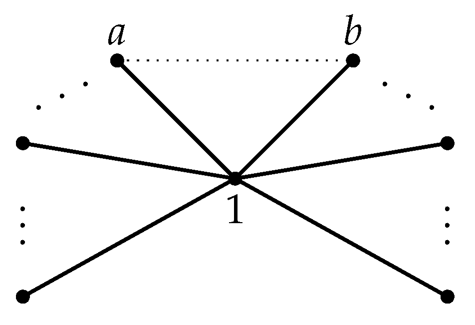
Lemma 13.
If , then the graph of W-algebra is a star graph.
Proof.
Let not be a star graph and . So, a and b are adjacent in where with and . Then, becomes a subgraph of as in Figure 4 such that and .
We have because a and 1 are adjacent. Therefore, it is obtained that . Then, we attain , similarly. Hence, .
Hence, does not contain elements a and b. Thus, it is obtained that . We get a contradiction with our hypothesis. □
Corollary 3.
The graph of equivalence classes, , consists of an edge if and only if is a star graph.
Lemma 14.
, the graph of equivalence classes, is a subgraph of .
Proof.
Suppose that . Using Definition 3 and Definition 7, we obtain that . Let . Then, we have . Since , we obtain , i.e., . Hence, we conclude that . Then, is a subgraph of . □
Lemma 15.
The elements a and 1 are adjacent in for each .
Proof.
We have for each . Accordingly, . This means that vertices a and 1 are adjacent. □
Theorem 5.
A star graph with vertex is a subgraph for every graph .
Proof.
By Lemma 15, we have for all . In other words, a is adjacent to vertex for each . The degree of the vertex is and the degree of the other vertices is 1 where . □
Theorem 6.
Let be the graph of equivalence classes of having any distinct vertices . If vertex and vertex are adjacent, then and become separated W-complement annihilators of .
Proof.
We suppose that . This means that a and b are in the same equivalence class. We get since and are adjacent. This implies that a and b are in different equivalence classes. This is a contradiction with our hypothesis. Then, it is obtained that , that is, and are distinct W-complement annihilators of . □
Theorem 7.
If W-graph is a complete graph, then is isomorphic to .
Proof.
We assume that . Elements of A correspond to vertices of by Definition 3. Then, we get for .
Since is a complete graph, two distinct vertices and are adjacent where . Accordingly, we have
for . Then, we get
for and . Consequently, each distinct vertex in coincides with a distinct equivalence class of .
Now, we describe a mapping between vertex sets of and as follows:
for . The mapping is an isomorphism between and .
Furthermore, we depict a mapping between edge sets of and as follows:
, the mapping of edges, is a well-defined bijection. is also a complete graph because is complete and is an isomorphic mapping between and . □
Lemma 16.
If consists of an edge, then this edge consists of two vertices such that and where for .
Proof.
We suppose that there exists an such that for any . Since , we get . For all , . So, must be distinct from . However, our assumption has led us to a contradiction. Therefore, there are no different equivalence classes like , which is equivalent to the equivalence class . Because the graphs of equivalence classes have one edge and two vertices, one of these vertices corresponds to the equivalence class , while the other vertex likewise corresponds to the equivalence class, which consists of all elements of the . □
Theorem 8.
W-graph is a complete bipartite graph if and only if consists of an edge.
Proof.
Since is a complete bipartite graph, there exist
such that and . Therefore, we get the following set of edges
We attain the following neighborhoods by using
and
Thus, we have for all and for all . This implies that there exist only two adjacent and distinct equivalence classes and in . Hence, consists of only one edge.
It is obvious from Lemma 16. □
Lemma 17.
Assume that is an isomorphism where and are two graphs of W-algebra. If for and , then .
Proof.
It is obvious. □
Theorem 9.
Suppose that and are two graphs of W-algebrasand , respectively. There also exists an isomorphism between and if there exists an isomorphism between and .
Proof.
We assume that there exists an isomorphism between and . As a result, an isomorphism exists as follows
such that , for all . We obtain , i.e., with the help of Lemma 17.
Herein, we describe a mapping between the edges of and such that
Hence, the mapping is a well-defined bijection. As a consequence, we attain that . □
Now, Algorithm 5 is developed to represent the graph of equivalence classes of .

The algorithm of determining the graph of equivalence classes of establishes the graph of equivalence classes of a W-algebra where the inputs are set A, → operation and ¬ operation (Algorithm 5, or EquivalenceGraph).
The algorithm investigates whether set A produces a W-algebra in lines 1–3. If A does not become a W-algebra, the algorithm is stopped. ∆ Cayley table is described with the ∆-Operation algorithm by using binary operation → and unary operation ¬ on set A in line 4. Then, in line 5, , the graph of , is specified using Graph algorithm. Following that, the Sets algorithm constructs a set of complement annihilators of each element in A and returns the set of complement annihilators to as neighborhood sets of each vertex in in line 6.
In accordance with this, line 7 initializes the vertex set of to V and the edge set to an empty set. Additionally, in lines 9–15, it is assessed that vertices have the same neighborhood sets for each . Such v vertices are demonstrated by u in the graph , and v is removed from . After that, in lines 16–19, it is checked whether . If , then the edge is added to . Finally, the EquivalenceGraph algorithm achieves , the graph of the equivalence classes of , in line 20 and prints this graph.
6. Conclusions
In this paper, we present an algorithmic strategy for building graphs by associating with W-algebras. On W-algebras, we introduce concepts such as ∆-connection operator and complement annihilator to achieve this goal. So far, the concept of annihilator has been used in graph structures created on algebras. The novelty of this work is that, because the W-algebra structure is limited with an upper bound, the concept of complement annihilator was introduced and W-graphs and graphs of equivalence classes were produced using this notion. Simultaneously, we provide algorithms to support our results gained throughout the paper. As a result, this paper attempts to build algorithms for researchers working in various fields of science who use W-algebras and graphs by employing a novel notion known as complement annihilating.
Funding
This research received no external funding.
Data Availability Statement
Not applicable.
Acknowledgments
I am grateful to Ege University Planning and Monitoring Coordination of Organizational Development and Directorate of Library and Documentation for their support in editing and proofreading service of this study.
Conflicts of Interest
The author declares no conflict of interest.
References
- Iampan, A. A new branch of the logical algebra: UP-algebras. J. Algebra Relat. Top. 2017, 5, 35–54. [Google Scholar]
- Kim, C.B.; Kim, H.S. On BG-algebras. Demonstr. Math. 2008, 41, 497–506. [Google Scholar] [CrossRef]
- Oner, T.; Kalkan, T.; Gursoy, N.K. Sheffer stroke BG-algebras. Int. J. Maps Math.-IJMM 2021, 4, 27–39. [Google Scholar]
- Rump, W. L-algebras, self-similarity, and l-groups. J. Algebra 2008, 320, 2328–2348. [Google Scholar] [CrossRef] [Green Version]
- Rump, W.; Yang, Y. Intervals in l-groups as L-algebras. Algebra Universalis 2012, 67, 121–130. [Google Scholar] [CrossRef]
- Traczyk, T. On the structure of BCK-algebras with zx· yx= zy· xy. Math. Japon 1988, 33, 319–324. [Google Scholar]
- Wang, J.; Wu, Y.; Yang, Y. Basic algebras and L-algebras. Soft Computing 2020, 24, 14327–14332. [Google Scholar] [CrossRef]
- Basnet, D.K.; Singh, L.B. fuzzy ideal of BG-algebra. Int. J. Algebra 2011, 5, 703–708. [Google Scholar]
- Smarandache, F.; Bordbar, H.; Borzooei, R.A.; Jun, Y.B. A general model of neutrosophic ideals in BCK/BCI-algebras based on neutrosophic points. Bull. Sect. Log. 2020, 50, 355–371. [Google Scholar] [CrossRef]
- Muhiuddin, G.; Al-Kadi, D.; Shum, K.P.; Alanazi, A.M. Generalized Ideals of BCK/BCI-Algebras Based on Fuzzy Soft Set Theory. Adv. Fuzzy Syst. 2021, 2021, 8869931. [Google Scholar] [CrossRef]
- Senapati, T.; Muhiuddin, G.; Shum, K.P. Representation of up-algebras in interval-valued intuitionistic fuzzy environment. Ital. J. Pure Appl. Math. 2017, 38, 497–517. [Google Scholar]
- Senapati, T.; Jun, Y.B.; Shum, K.P. Cubic set structure applied in UP -algebras. Discret. Math. Algorithms Appl. 2018, 10, 18500490. [Google Scholar] [CrossRef]
- Subha, V.S.; Dhanalakshmi, P. New type of fuzzy ideals in BCK/BCI algebras. World Sci. News 2021, 153, 80–92. [Google Scholar]
- Wu, Y.; Wang, J.; Yang, Y. Lattice-ordered effect algebras and L-algebras. Fuzzy Sets Syst. 2019, 369, 103–113. [Google Scholar] [CrossRef]
- Rose, A.; Rosser, J.B. Fragments of Many-Valued Statement Calculi. Trans. Am. Math. Soc. 1958, 87, 1–53. [Google Scholar] [CrossRef]
- Salas, A.J.R. Un Estudio algebraico de los cálculos proposicionales de Lukasiewicz. Ph.D. Thesis, Universitat de Barcelona, Barcelona, Spain, 1980. [Google Scholar]
- Chang, C.C. Algebraic Analysis of Many Valued Logics. Source Trans. Am. Math. Soc. 1958, 88, 467–490. [Google Scholar] [CrossRef]
- Chang, C.C. A New Proof of the Completeness of the Lukasiewicz Axioms. Trans. Am. Math. Soc. 1959, 93, 74. [Google Scholar] [CrossRef]
- Font, J.M.; Rodríguez, A.J.; Torrens, A. Wajsberg algebras. Stochastica 1984, 8, 5–31. [Google Scholar]
- Ahamed, M.B.; Ibrahim, A. Fuzzy implicative filters of lattice Wajsberg Algebras. Adv. Fuzzy Math. 2011, 6, 235–243. [Google Scholar]
- Ahamed, M.B.; Ibrahim, A. Anti fuzzy implicative filters in lattice W-algebras. Int. J. Comput. Sci. Math. 2012, 4, 49–56. [Google Scholar]
- Anderson, D.D.; Naseer, M. Beck’s coloring of a commutative ring. J. Algebra 1993, 159, 500–514. [Google Scholar] [CrossRef] [Green Version]
- Anderson, D.F.; Livingston, P.S. The zero-divisor graph of a commutative ring. J. Algebra 1999, 217, 434–447. [Google Scholar] [CrossRef] [Green Version]
- Atani, S.E.; Saraei, F.E.K. The total graph of a commutative semiring. Analele Stiintifice Ale Univ. Ovidius Constanta Ser. Mat. 2013, 21, 21–33. [Google Scholar] [CrossRef] [Green Version]
- Beck, I. Coloring of commutative rings. J. Algebra 1988, 116, 208–226. [Google Scholar] [CrossRef]
- Birch, L.M.; Thibodeaux, J.J.; Tucci, R.P. Zero Divisor Graphs of Finite Direct Products of Finite Rings. Commun. Algebra 2014, 42, 3852–3860. [Google Scholar] [CrossRef]
- DeMeyer, F.R.; McKenzie, T.; Schneider, K. The Zero-divisor Graph of a Commutative Semigroup. Semigroup Forum 2002, 65, 206–214. [Google Scholar] [CrossRef]
- DeMeyer, F.; DeMeyer, L. Zero divisor graphs of semigroups. J. Algebra 2005, 283, 190–198. [Google Scholar] [CrossRef] [Green Version]
- Anderson, D.F.; Badawi, A. The total graph of a commutative ring. J. Algebra 2008, 320, 2706–2719. [Google Scholar] [CrossRef] [Green Version]
- Talebi, Y.; Darzi, A. On graph associated to co-ideals of commutative semirings. Comment. Math. Univ. Carol. 2017, 58, 293–305. [Google Scholar] [CrossRef]
- Maimani, H.R.; Yassemi, S. On the zero-divisor graphs of commutative semigroups. Houst. J. Math. 2011, 37, 733–740. [Google Scholar]
- Chelvam, T.T.; Nithya, S. Zero-divisor graph of an ideal of a near-ring. Discret. Math. Algorithms Appl. 2013, 5, 1350007. [Google Scholar] [CrossRef]
- Akram, M.; Samanta, S.; Pal, M. Cayley vague graphs. J. Fuzzy Math 2017, 25, 449–462. [Google Scholar]
- Mulay, S.B. Cycles and symmetries of zero-divisors. Commun. Algebra 2002, 30, 3533–3558. [Google Scholar] [CrossRef]
- Redmond, S.P. The zero-divisor graph of a non-commutative ring. Int. J. Commut. Rings 2002, 1, 203–211. [Google Scholar]
- Božić, I.; Petrović, Z. Zero-divisor graphs of matrices over commutative rings. Commun. Algebra 2009, 37, 1186–1192. [Google Scholar] [CrossRef]
- Akbari, S.; Ghandehari, M.; Hadian, M.; Mohammadian, A. On commuting graphs of semisimple rings. Linear Algebra Its Appl. 2004, 390, 345–355. [Google Scholar] [CrossRef] [Green Version]
- Akbari, S.; Bidkhori, H.; Mohammadian, A. Commuting graphs of matrix algebras. Commun. Algebra 2008, 36, 4020–4031. [Google Scholar] [CrossRef]
- Akbari, S.; Mohammadian, A.; Radjavi, H.; Raja, P. On the diameters of commuting graphs. Linear Algebra Its Appl. 2006, 418, 161–176. [Google Scholar] [CrossRef] [Green Version]
- Dolinar, G.; Guterman, A.; Kuzma, B.; Oblak, P. Commuting graphs and extremal centralizers. Ars Math. Contemp. 2014, 7, 453–459. [Google Scholar] [CrossRef]
- Bakhadly, B.R. Orthogonality graph of the algebra of upper triangular matrices. Oper. Matrices 2017, 11. [Google Scholar] [CrossRef] [Green Version]
- Bakhadly, B.R.; Guterman, A.E.; Markova, O.V. Graphs defined by orthogonality. J. Math. Sci. (United States) 2015, 207, 698–717. [Google Scholar] [CrossRef]
- Guterman, A.E.; Markova, O.V. Orthogonality Graphs of Matrices Over Skew Fields. J. Math. Sci. 2018, 232, 797–804. [Google Scholar] [CrossRef]
- Afkhami, M.; Khashyarmanesh, K.; Rajabi, Z. Some results on the annihilator graph of a commutative ring. Czechoslov. Math. J. 2017, 67, 151–169. [Google Scholar] [CrossRef]
- Ebrahimi, S.; Nikandish, R.; Tehranian, A.; Rasouli, H. On the Strong Metric Dimension of Annihilator Graphs of Commutative Rings. Bull. Malays. Math. Sci. Soc. 2021, 44, 2507–2517. [Google Scholar] [CrossRef]
- Gursoy, A.; Kircali Gursoy, N.; Oner, T.; Senturk, I. An alternative construction of graphs by associating with algorithmic approach on MV-algebras. Soft Comput. 2021, 25, 13201–13212. [Google Scholar] [CrossRef]
- Cignoli, R.L.; d’Ottaviano, I.M.; Mundici, D. Algebraic Foundations of Many-Valued Reasoning; Springer Science & Business Media: Dordrecht, The Netherlands, 2013; Volume 7. [Google Scholar]
- Chang, C.C. The writing of the MV-algebras. Stud. Log. Int. J. Symb. Log. 1998, 61, 3–6. [Google Scholar]
- Chartrand, G.; Lesniak, L.; Zhang, P. Graphs & Digraphs; Chapman and Hall/CRC: New York, USA, 2010. [Google Scholar] [CrossRef]
- Harary, F. Graph Theory; Addison-Wesley Publishing Company: Reading, MA, USA, 1969; p. 274. [Google Scholar]
Figure 1.
of Example 2.

Figure 2.
of Example 3.

Figure 3.
Graph of Example 4.

Figure 4.
Subgraph of .

Disclaimer/Publisher’s Note: The statements, opinions and data contained in all publications are solely those of the individual author(s) and contributor(s) and not of MDPI and/or the editor(s). MDPI and/or the editor(s) disclaim responsibility for any injury to people or property resulting from any ideas, methods, instructions or products referred to in the content. |
© 2023 by the author. Licensee MDPI, Basel, Switzerland. This article is an open access article distributed under the terms and conditions of the Creative Commons Attribution (CC BY) license (https://creativecommons.org/licenses/by/4.0/).
Share and Cite
MDPI and ACS Style
Kırcalı Gürsoy, N. Graphs of Wajsberg Algebras via Complement Annihilating. Symmetry 2023, 15, 121. https://doi.org/10.3390/sym15010121
AMA Style
Kırcalı Gürsoy N. Graphs of Wajsberg Algebras via Complement Annihilating. Symmetry. 2023; 15(1):121. https://doi.org/10.3390/sym15010121
Chicago/Turabian StyleKırcalı Gürsoy, Necla. 2023. "Graphs of Wajsberg Algebras via Complement Annihilating" Symmetry 15, no. 1: 121. https://doi.org/10.3390/sym15010121
Note that from the first issue of 2016, this journal uses article numbers instead of page numbers. See further details here.