Malware Detection Using Deep Learning and Correlation-Based Feature Selection

Abstract

Malware is one of the most frequent cyberattacks, with its prevalence growing daily across the network. Malware traffic is always asymmetrical compared to benign traffic, which is always symmetrical. Fortunately, there are many artificial intelligence techniques that can be used to detect malware and distinguish it from normal activities. However, the problem of dealing with large and high-dimensional data has not been addressed enough. In this paper, a high-performance malware detection system using deep learning and feature selection methodologies is introduced. Two different malware datasets are used to detect malware and differentiate it from benign activities. The datasets are preprocessed, and then correlation-based feature selection is applied to produce different feature-selected datasets. The dense and LSTM-based deep learning models are then trained using these different versions of feature-selected datasets. The trained models are then evaluated using many performance metrics (accuracy, precision, recall, and F1-score). The results indicate that some feature-selected scenarios preserve almost the same original dataset performance. The different nature of the used datasets shows different levels of performance changes. For the first dataset, the feature reduction ratios range from 18.18% to 42.42%, with performance degradation of 0.07% to 5.84%, respectively. The second dataset reduction rate is between 81.77% and 93.5%, with performance degradation of 3.79% and 9.44%, respectively.

1. Introduction

Malware has affected a lot of computing gadgets in the digital age. Malevolent software, or malware, is created with the intention of achieving the negative goals of a malicious attacker. Malware can attack networks, damage vital infrastructure, compromise computers and smart devices, and steal sensitive data [1].

The modern idea of an information society has evolved thanks to the Internet of Things (IoT) and its applications. However, security issues provide a significant barrier to achieving the advantages of this industrial development as cybercriminals target specific PCs and networks in order to steal private information for financial gain and disrupt systems [2]. Such attackers utilize malicious software, or “malware,” to expose system vulnerabilities and pose substantial hazards. Computer software designed to harm the operating system is known as malware (OS) [3]. These malware attacks have increased significantly since our daily interactions have undergone a significant transformation as a result of the development of mobile technology. Online learning, social networking, online banking, online shopping, and web browsing are a few examples of services offered by mobile devices while connected to the Internet. Mobile gadgets have therefore played a key role and have evolved into a necessary aspect of daily life [4]. In total, 4.78 billion people worldwide are using mobile devices as of 2020 [5]. These mobile devices do make life more convenient for consumers, but they are also vulnerable to virus invasion and attacks because of online social networks and services. Mobile malware is capable of disguising itself as ordinary code and then altering any intended program to corrupt and obstruct the operation of the system [5,6,7].

A permission-based approach has been offered by Google Play as a security measure to prevent the application from obtaining private data. By taking into account the assets of the application that have been accessed, this permission prompts users prior to installation. Before moving forward with the installation, the users must expressly accept the agreement. Unfortunately, the Google Play method cannot fully safeguard the user because they have a tendency to accept the agreement without carefully reading the authorization [5,8]. Another threat possibility can come from profiting off successful Android apps, as seen by the over 10-fold increase in Android malware detections between 2012 and 2018 [9]. Furthermore, every day in 2018, there were over 12 K brand-new Android malware samples found. The recently revealed Android malware samples are more advanced than the ones that first surfaced a few years ago in terms of escaping anti-virus monitoring through coding and encryption, in addition to the rapid proliferation of malware [10,11].

Malware detection studies utilizing machine learning are growing in popularity because they are a successful strategy that can produce a high level of detection accuracy [12]. Some previous studies utilized machine learning (ML) algorithms, which can make decisions after learning from the data templates. Machine learning is the concept of minimizing human intervention in computing systems [13]. Through the use of computer learning methodologies and experience or previous data, machine learning predicts decisions. To analyze the features and track the model, there are supervised and unsupervised learning methods [14,15]. In both cases, the machine learns to distinguish between malicious and benign activities. In supervised learning, the ML model is given the input and targets together and learns to always match the actual malware patterns with their corresponding “malware” classes and match the normal activities with the “normal” classes. The training process is repeated until the model learns to correctly predict all samples [5]. Many ML algorithms have been used, like support vector machines (SVM) [16,17,18], K-nearest neighbor (KNN) [19,20], Bayesian estimation [21,22], genetic algorithms [23], etc., in order to build malware detection systems. Unsupervised learning methods provide the inputs without any targets, and the ML algorithm is learned to distinguish between malware and benign samples. However, some studies fused the supervised and unsupervised learning methodologies together [24].

Malware detection is an important security topic with strong associations with firms’ legal, reputational, and economic concerns. Deep learning as a method for making and fixing detection mechanisms is a good way to solve many problems with how to detect malware. But when it comes to deep learning, there are many difficult things that need to be considered when thinking about detection mechanisms. Correlation-based feature selection, the dense layer model, and the LSTM model are presented as three challenging and symmetric ways to affect performance.

In the current research, two different datasets will be used. One of them contains a large number of records, while the other one consists of a large number of predictors (attributes). The feature selection of the best attributes will be used in many scenarios in order to define the best combination of attributes. The correlation with the target attribute “classification” will be used as the feature selection methodology. In the training step, the Dense and LSTM models will be used and compared, so that many training scenarios will be configured depending on different feature selection criteria, different splitting criteria, and different dataset architectures. Our main contribution is using the efficiency of deep learning and feature selection methodologies in the malware detection field in order to build a robust, powerful, low-computational malware detection system.

Related Work

Some of the previous studies used machine learning (ML) approaches, while others applied deep learning (DL) techniques, including convolutional networks (CNN), recurrent neural networks (RNN), and long-short-term memory networks (LSTM) [25,26,27]. Some of them used desktop-related malware datasets, but most took care of the mobile-related malware datasets.

Many machine learning and deep learning models were used for malware detection, according to Vinayakumar et al. [3]. They used the Ember malware dataset, consisting of 70,140 benign and 69,869 malware recodes. Several ML and DL models were applied (KNN, SVM, Random Forests (RF), AdaBoost, Logistic Regression (LR), Naïve Bayes (NB), and Deep Neural Network (DNN)). They used the Adam optimization algorithm, and the models were trained for 200 epochs. The best result was obtained by the LSTM model with 98.9% accuracy.

A malware detection system based on DL was introduced by Jeon and Moon in 2020 [25]. They used the convolutional encoder to translate the opcode sequences extracted from Windows executable files. The recurrent neural networks (RNNs) were then used for the malware detection process. Their approach achieved 96% detection accuracy and a 95% true positive rate.

In another study by Yazdinejad et al. [26], opcodes for malware and benign activities were extracted from a dataset of 200 benign and 500 malware records. They applied the LSTM model to build a malware detection system using 10-fold cross-validation on the acquired dataset. Their study achieved a detection accuracy of 98%.

Opcodes and system calls were used in a study by Darabian et al. [27]. The total collected dataset contains 1500 executable samples, and the CNN-LSTM model was trained using this dataset. The opcodes-based collected records achieved a detection accuracy of 99%, while the system calls achieved only a 95% detection rate.

Hwang et al. [28] proposed a malware detection system based on a malware dataset consisting of 10,000 malware records and 10,000 benign files. The DNN is trained using this dataset (80% for training and 20% for testing). Their proposed system achieved 94% accuracy.

Ban et al. [29] used convolutional neural networks (CNN) for the Android malware detection process. They used a malware dataset consisting of 28,179 records of the most malware activities that appeared from 2018 to 2020. The experiments showed that their approach achieved 98% accuracy and a 0.82 F1-score.

The “wrapping feature selection” (WFS) method was proposed in a study by Smmarwar et al. [30]. They used random forests, decision trees, and SVM classifiers. Those classifiers are trained using the optimal number of selected features from the CIC-InvesAndMal2019 malware dataset. The experiments showed that the SVM, RF, and DT models achieved 82.33%, 91.32%, and 91.8% accuracy, respectively.

Toan et al. [31] used the static opcode features of the MIPS ELF malware dataset, consisting of 4511 malware and 4393 benign activities. They used the machine learning models on the Internet of Things (IoT) platforms for malware detection. Their models achieved an accuracy of 99.8% using only 20 opcodes.

Our study will use the feature selection approach to minimize the number of features (columns), reducing the next computational time. Besides, the proposed correlation-based approach helps selecting the best features, improving performance. The combination of deep learning, high performance, and feature selection will result in a robust, low computational, and powerful malware detection model that was not introduced by any of the previous studies.

2. Materials and Methods

2.1. Datasets

Two different datasets are used in the current study. In the first dataset, the main feature is the large number of records, while the main feature of the second dataset is the high dimensionality (large number of attributes).

2.1.1. First Dataset (Malware Detection)

The network traffic of a virtual machine on a Unix/Linux-based platform was used to build this dataset. The dataset includes the harmless actions of malware software for Android devices. It consists of 35 attributes (features) and 100,000 records (50,000 malware records and 50,000 benign ones). The dataset was created for classification and malware detection purposes.

Table 1. First malware dataset description.

No.	Attribute/Type	Description	Type
1.	Hash	APK/ SHA256 file name	Text
2.	Millisecond/ number	Time	number
3.	Classification	Malware or benign	Text
4.	State	State of the tasks (non-runnable, runnable or stopped)	number
5.	usage_counter	task structure usage counter	number
6.	prio	Holds the dynamic priority of a task	Number
7.	Static_prio	Static priority of a task	Number
8.	normal_prio	Normal Priority (without taking into account the RT-inheritance)	Number
9.	Policy	Task planning policy	Number
10.	vm_pgoff	Offset of the area in the file (in pages)	Number
11.	vm_truncate_count	used to mark a vma as now dealt with	Number
12.	task_size	Current task size	Number
13.	cached_hole_size	Free address space hole size	Number
14.	free_area_cache	First address of space hole	Number
15.	mm_users	Space users	Number
16.	map_count	Count of memory areas	Number
17.	hiwater_rss	Peak of resident set size	Number
18.	total_vm	Total number of pages	Number
19.	shared_vm	shared pages count	Number
20.	exec_vm	Executable pages count	Number
21.	reserved_vm	Reserved pages count	Number
22.	nr_ptes	Page table entries count	Number
23.	end_data	End address of code component	Number
24.	last_interval	Last interval time before thrashing	Number
25.	Nvcsw	Volunteer context switches count	Number
26.	Nivcsw	in-volunteer context switches count	Number
27.	min_flt	Minor faults (page faults)	Number
28.	maj_flt	Major faults (page faults)	Number
29.	fs_excl_counter	Count of file system exclusive resources	Number
30.	Lock	Read-write synchronization lock which is used for file system access	Number
31.	Utime	User time	Number
32.	Stime	System time	Number
33.	Gtime	Guest time	Number
34.	Cgtime	Cumulative group time	Number
35.	signal_nvcsw	Cumulative resource counter	Number

includes detailed information about the attributes of this dataset. The dataset is available on the Kaggle site [32].

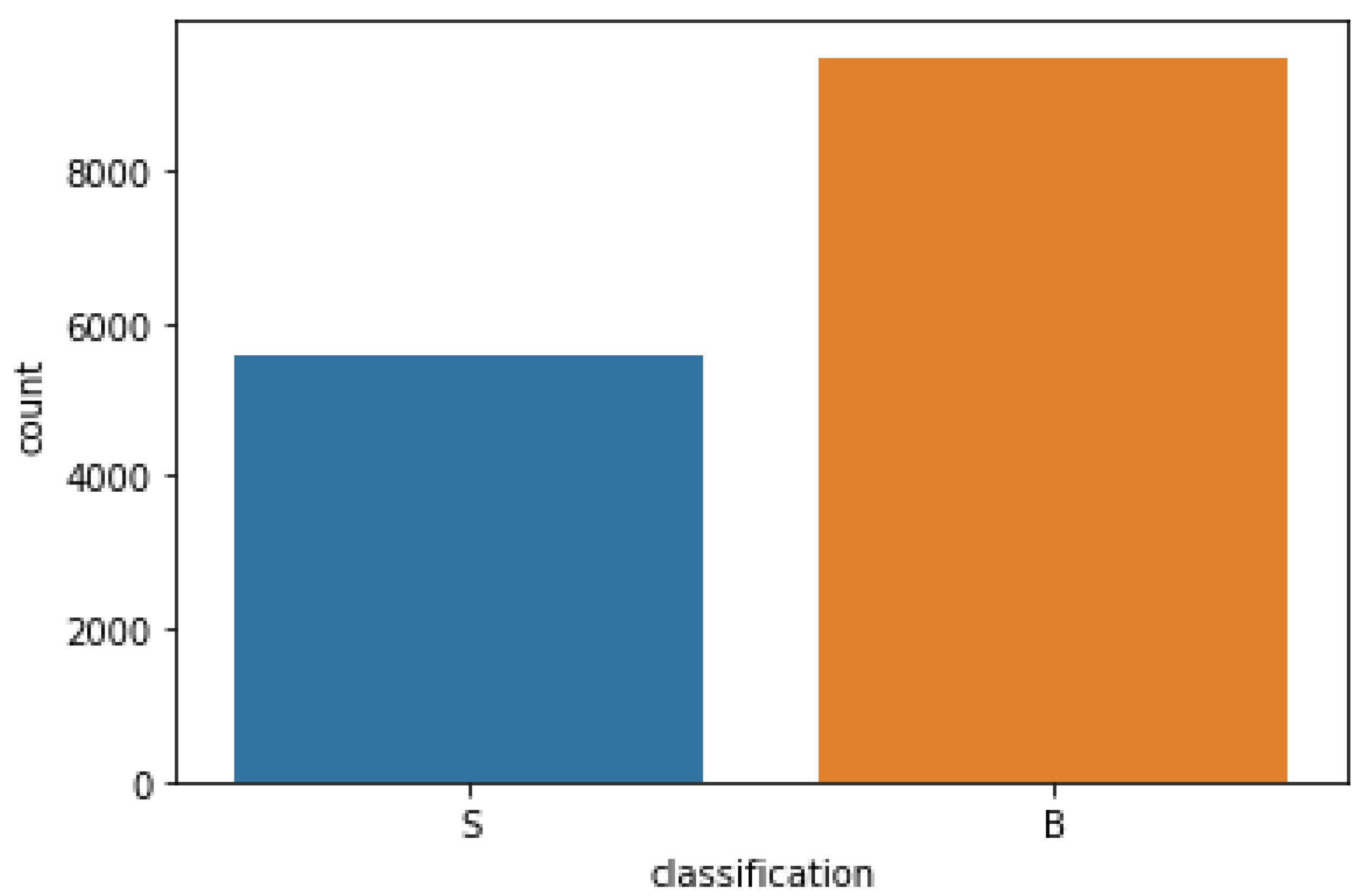
2.1.2. Second Dataset (Android Malware Dataset for Machine Learning)

This dataset is available on the Kaggle site [33]. It is made up of 215 distinct attributes gathered from over 15,000 Android applications (9476 benign and 5560 malicious) [34]. Figure 1 shows the distribution of the benign and malware classes through this dataset.

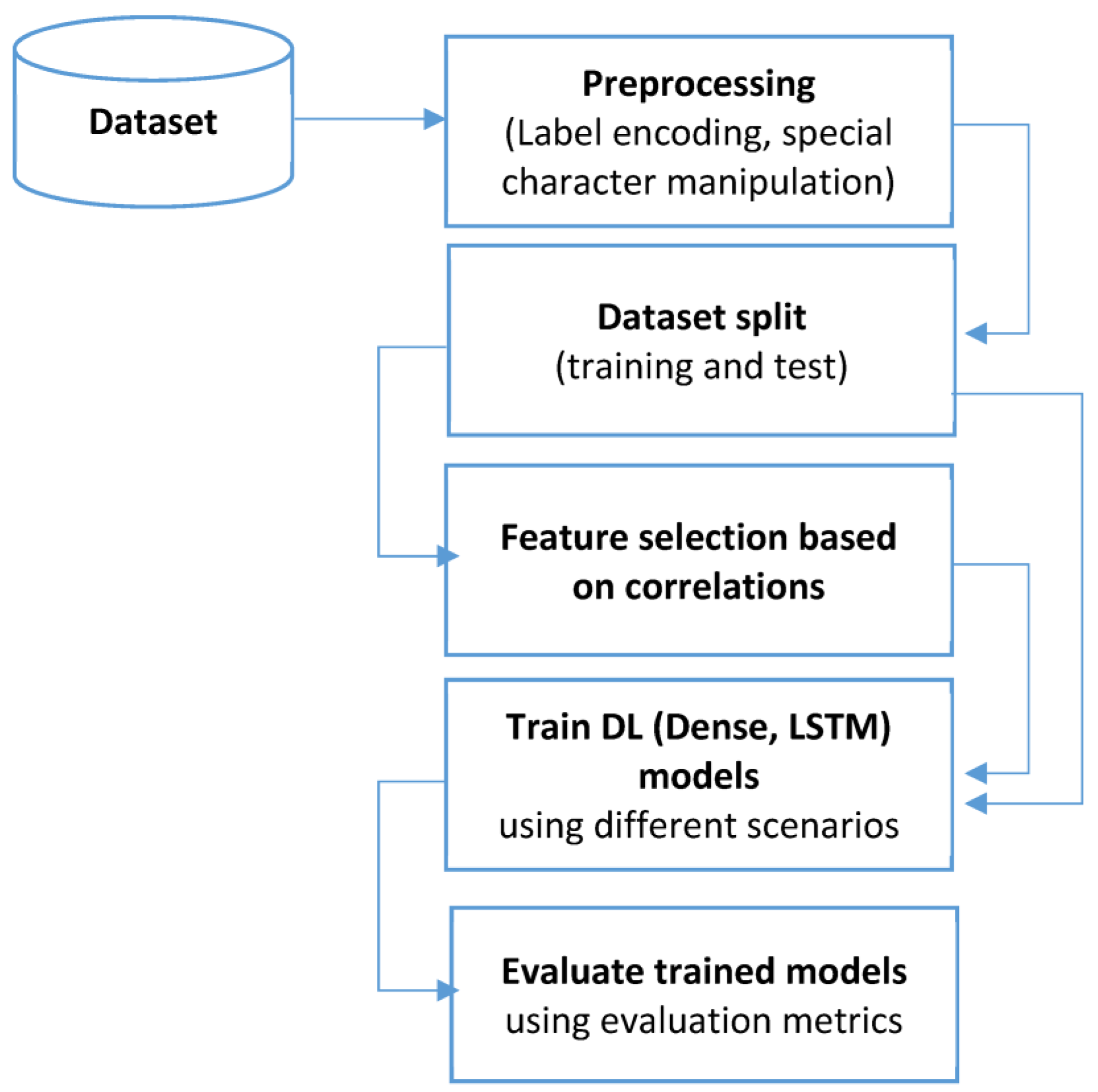
2.2. Proposed Methodology

In this study, many DL methods are proposed and used. In order to train the DL models using the two selected datasets, these datasets need a preprocessing step in which the classification (target) columns are encoded (numbered) and the special characters or missed values are processed. Since the two datasets differ in their nature, the preprocessing steps will be somehow different.

After preprocessing the datasets, they are split into training and test sets. In some training scenarios, the feature selection process is performed before the training process in order to minimize the data dimensionality (computational time).

After that, the DL models will be built and trained based on many training scenarios, including different splitting criteria, different DL architectures, and with or without feature selection. Figure 2 illustrates the proposed methodology for both datasets.

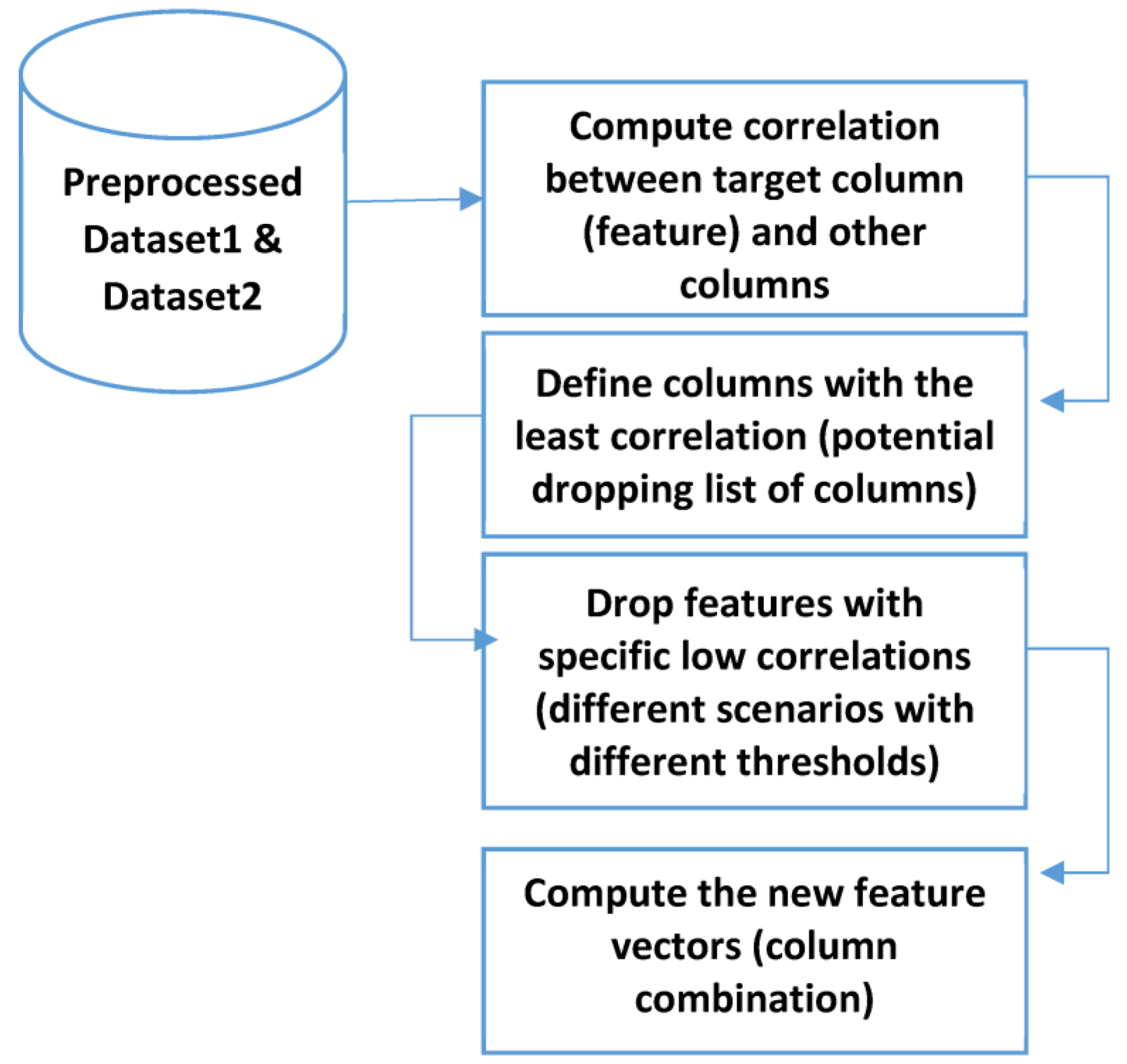
2.2.1. Correlation-Based Feature Selection

The goal of feature selection is to select the best features of the studied problem in order to reduce computational time. However, in our study, a correlation-based approach is proposed in order to minimize the high dimensionality, reduce the computational time, and select the best combinations of features so that the performance of the training and evaluation process will be increased. Figure 3 illustrates the correlation-based feature selection approach.

For the first dataset, the correlations between all columns and the target column are computed using Equation (1).

$$Cor{r}_{x,y}=\frac{\sum \left(x_i-\overline{x}\right) \left(y_i-\overline{y}\right)}{\sqrt{\sum {\left(x_i-\overline{x}\right)}^2{\left(y_i-\overline{y}\right)}^2 }}$$

(1)

where, Corr_xy is the correlation between feature x_i and target feature y. $\overline{x}$ and $\overline{y}$ are the mean value of x and y, respectively.

Then a list of potential dropped columns is prepared. Different selection scenarios can be made since the correlation ranges between 0 and 1. The selection step is based on the number of desired columns, so we will obtain the K number of required features and drop the rest. For the second dataset, the same approach will be applied except for the selection step. Specific correlation thresholds (T) will be used to eliminate columns since the number of columns in the second dataset is 214. So, in the second dataset, the number of selected features depends on the chosen threshold, which is not defined as in the first dataset.

2.2.2. Dense Layers Model

In the current study, we suggest using the dense-based architecture with hidden layers of 50 neurons for the first dataset scenarios and 100 neurons for the second dataset scenarios (since the second dataset has 214 attributes while the first one has only 33). The first dense layer is the input layer, with an input size equal to the number of selected features (this number varies depending on each scenario). The activation function of the first layer is the “relu” non-linear function. The next five layers are the hidden dense layers, with 50 cells each and a “relu” activation function. The last dense layer is the output layer, with two outputs and a “softmax” activation function. The “softmax” function is necessary for the last layer since we need an activation function that produces probabilities for all possible outputs (malware and benign), and then the class with the highest probability is chosen as the final prediction.

We chose five hidden layers after applying many experiments to find the best number of hidden layers. After five hidden layers, the performance stops getting better, so we choose “five” as the right number of hidden layers.

Our proposed model is very simple in order to minimize the number of learnable parameters. Unlike in previous studies, experiments are used to figure out the number of neurons and the number of hidden layers in order to find the best combination for the problem being studied.

2.2.3. LSTM Model

For the LSTM proposed model, the first dense layer is replaced by an LSTM layer “relu” activation function. The rest of the dense and output layers are left the same as the previous dense model. By replacing the dense layer with the LSTM layer, the number of parameters that can be learned will increase by a lot. As a result, the training time will increase.

2.2.4. Evaluation Criteria

The evaluation step is the last part in which the performance evaluation is done using many metrics. In this study, the validation accuracy, test accuracy, training time, precision, recall, and F1-score are used for the performance evaluation step.

The validation accuracy is computed through the training process by testing the trained model using the validation set. On the other hand, the test accuracy is calculated after the training, and it is used to test the trained model’s ability to tell the difference between new malware and harmless samples.

Four different calculations are used to figure out the precision, recall, and F1-score. (TP stands for true positives, TN for true negatives, FP for false positives, and FN for false negatives.)

These four statistics are computed as follows:

TP is the number of correctly classified malware samples among all malware samples. FN, on the other hand, is the opposite concept of TP and represents the number of incorrectly rejected malware samples that are predicted as benign samples. The number of correctly rejected benign samples (that are actually benign samples and correctly predicted as benign) is denoted by TN. On the other hand, FP is the opposite concept of TN and is calculated as the number of incorrectly accepted benign samples that must be rejected and considered benign samples (benign samples incorrectly classified as malware). The best performance is registered when the TP and TN have the highest values or when the FP and FN have the lowest values. Precision, recall, and F1-score are calculated as Equations (2)–(4) show [35].

Precision = TP/(TP + FP)

(2)

Recall = TP/(TP + FN)

(3)

F1-score= 2 × Precision × Recall/(Precision + Recall)

(4)

The precision concept represents the positive predictive value of the trained model, while the recall expresses its sensitivity. A high precision value means that the trained model can predict the positive class samples well (the malware samples are predicted very well, and the incorrectly accepted benign samples are low). The high recall value means that the sensitivity of the trained model to correctly reject the benign samples is very high. The high rates of precision and recall result in a high F1-score value, which expresses a mixed concept of precision and recall. To judge a trained model and see how well it works, the above statistics need to be calculated.

3. Results and Discussion

3.1. Dataset Preprocessing

The preprocessing step includes the following tasks:

• Handle the special characters by replacing them with “NaN” values.
• Check for the missing values and “NaN” values and replace them.
• Label the target class (classification column) using 0 for benign and 1 for malware.
• Drop column “hash” in the malware dataset.

3.2. Dataset Split

Split the dataset into training and testing using three splitting scenarios:

80% for training and 20% for test sets.

75% for training and 25% for test sets.

70% for training and 30% for test sets.

3.3. Feature Selection

For the first dataset, there are 35 attributes (including the target). The correlation between the target attribute “classification” and other attributes is computed in order to define the degree of importance of these attributes in the final prediction.

Table 2. Correlation between target column (classification) and the closest 20 columns of the malware dataset.

Attribute/Type	Correlation with Target Column
Prio	0.100359
last_interval	0.006952
min_flt	0.003069595
Millisecond	−2.479903 × 10−17
Gtime	−1.441608 × 10−2
Stime	−4.203713 × 10−2
free_area_cache	−5.123678 × 10−2
total_vm	−5.929110 × 10−2
State	−6.470178 × 10−2
mm_users	−9.364091 × 10−2
reserved_vm	−1.186078 × 10−1
fs_excl_counter	−1.378830 × 10−1
Nivcsw	−1.437912 × 10−1
exec_vm	−2.551234 × 10−1
map_count	−2.712274 × 10−1
static_prio	−3.179406 × 10−1
end_data	−3.249535 × 10−1
maj_flt	−3.249535 × 10−1
shared_vm	−3.249535 × 10−1
vm_truncate_count	−3.548607 × 10−1
Utime	−3.699309 × 10−1
Nvcsw	−3.868893 × 10−1

includes the correlation results of the first malware dataset (in decreasing order).

Table 2 shows that there are many columns that can be excluded since their correlations with the target column (the prediction column) are very weak.

In our study, for the first malware dataset, we will apply experiments based on four different scenarios. All these proposed scenarios are derived from the dropping of some columns (features). The dropping approach is based on the correlation between each of the columns (features) and the target column (class). Those correlations are placed in Table 2 for dataset 1 and

Table 3. Correlation between second malware dataset columns and the target column using a correlation-threshold of 0.1.

Attribute (Column)	Correlation Threshold = 0.1	Exist with Threshold = 0.2?
send_sms	0.546075	Yes
android.telephony.smsmanager	0.435190	Yes
read_phone_state	0.409344	Yes
receive_sms	0.388328	Yes
read_sms	0.370336	Yes
android.intent.action.boot_completed	0.314303	Yes
telephonymanager.getline1number	0.305944	Yes
write_sms	0.267501	Yes
write_history_bookmarks	0.242250	Yes
telephonymanager.getsubscriberid	0.241551	Yes
android.telephony.gsm.smsmanager	0.241038	Yes
install_packages	0.235660	Yes
read_history_bookmarks	0.231044	Yes
Internet	0.204219	Yes
access_location_extra_commands	0.197165	No
write_apn_settings	0.193827	No
Abortbroadcast	0.191727	No
Createsubprocess	0.185971	No
telephonymanager.getdeviceid	0.179910	No
receive_boot_completed	0.159870	No
restart_packages	0.157646	No
Chmod	0.146465	No
telephonymanager.getsimserialnumber	0.135075	No
Packageinstaller	0.113861	No
Remount	0.112943	No
Senddatamessage	0.110062	No
Chownz	0.107540	No

for dataset 2.

1-

First selected group (Dropping the following columns): ‘vm_truncate_count’, ‘shared_vm’, ‘exec_vm’, ‘nvcsw’, ‘maj_flt’, and ‘utime’, getting in only 27 attributes (since ‘classification’ and ‘Hash’ columns are already removed. The dropped columns are chosen from the columns whose correlation with the target column is low.

2-

Second selected group (Dropping the following columns): ‘vm_truncate_count’, ‘shared_vm’, ‘exec_vm’, ‘nvcsw’, ‘maj_flt’, ‘utime’, ‘static_prio’, ‘map_count’, and ‘end_data’, getting in only 24 attributes. Three new columns with low correlation to the target column are also dropped in addition to the previous dropping list of the first scenario.

3-

Third selected group (Dropping the following columns): ‘vm_truncate_count’, ‘shared_vm’, ‘exec_vm’, ‘nvcsw’, ‘maj_flt’, ‘utime’, ‘static_prio’, ‘map_count’, ‘end_data’, ‘nivcsw’, ‘fs_excl_counter’, and ‘reserved_vm’, getting in only 21 attributes. Again, in this scenario, three columns with low correlation are dropped.

4-

Forth selected group (Dropping the following columns): ‘vm_truncate_count’, ‘shared_vm’, ‘exec_vm’, ‘nvcsw’, ‘maj_flt’, ‘utime’, ‘static_prio’, ‘map_count’, ‘end_data’, ‘nivcsw’, ‘fs_excl_counter’, ‘reserved_vm’, ‘mm_users’, ‘state’, ‘total_vm’, ‘free_area_cache’, ‘stime’, ‘gtime’, and ‘millisecond’ getting in only 14 attributes.

While for the second “Android malware dataset,” the correlation between the target column and the other attributes of the dataset was also computed. Because of the large number of attributes in the second dataset, we followed a feature selection technique based on various correlation thresholds [36].

Using a correlation threshold of 0.1, the selected attributes are only 27 columns out of 214 (after removing the classification column). Table 3 shows the 27 selected attributes (columns) with their corresponding correlations. While using a correlation threshold of 0.2, the number of selected columns will be 14. As shown in Table 3, almost half of the columns are dropped at a threshold of 0.2. Using a threshold of 0.5 will result in only 39 features with a selection rate of 18.22%.

3.4. Training Scenarios

In the training step, many training scenarios are suggested based on many concepts (with or without feature selection, with or without an LSTM layer, using different feature selection thresholds, using different splitting criteria, etc.).

The training scenarios of the first malware dataset are:

-

Train a dense layer-based DL model using the original dataset and different selected groups of dataset features (there are four groups and the original dataset, which means five different scenarios).

-

Train the DL model that has been modified (an LSTM layer has been added) using the first set of features that were chosen.

-

Train the DL model using three different splitting criteria (two new scenarios).

The training scenarios of the second malware dataset are:

-

Train a dense layer-based DL model with the original dataset and the three groups of selected features (four different scenarios).

-

Train the modified DL model (added LSTM layer) using the main dataset.

-

Train the DL model using different spitting criteria (two new scenarios).

A total of 12 different training scenarios are done in order to identify the effects of using different datasets, different feature selection options, different splitting criteria, and different DL architectures.

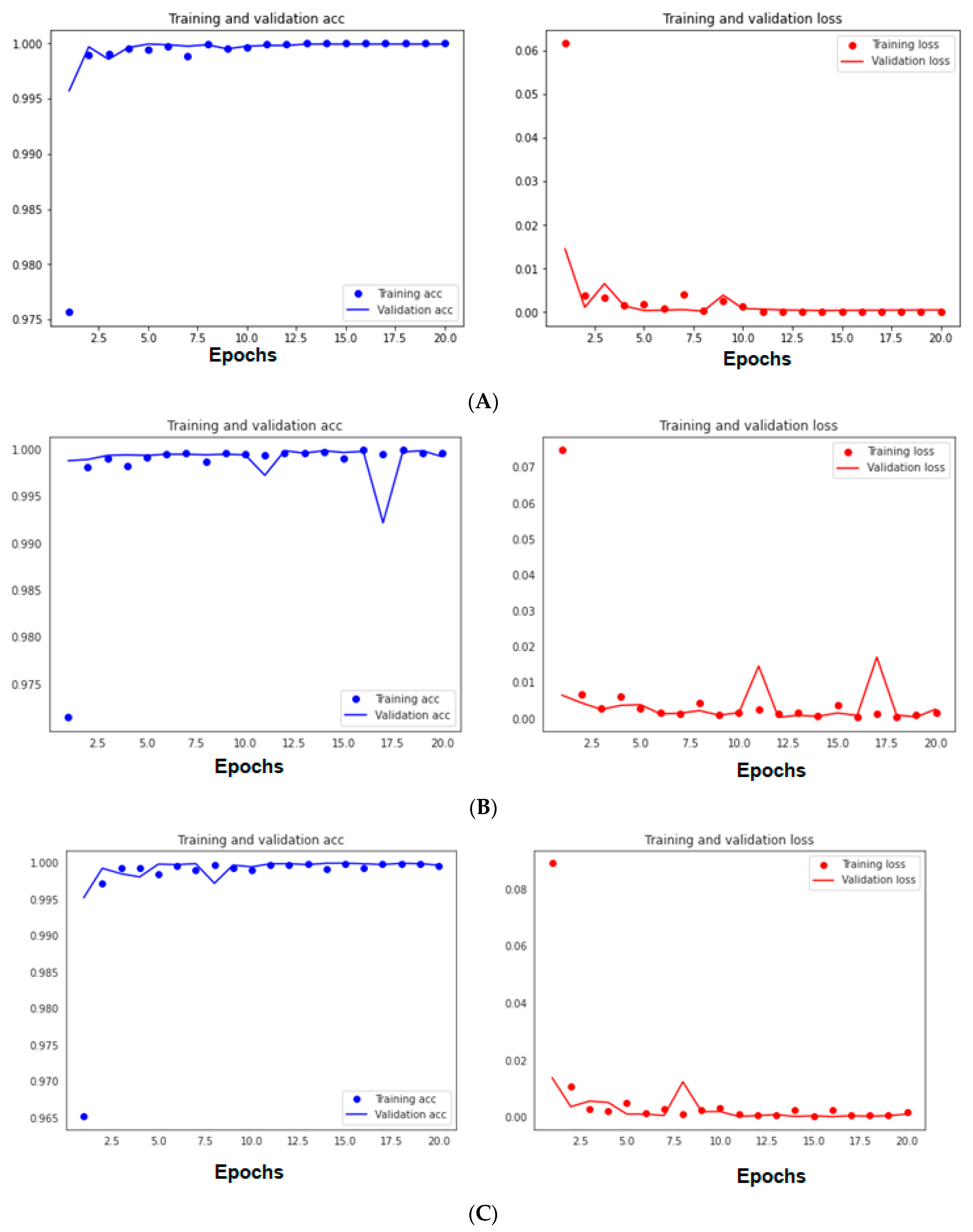
3.5. Experimental Results

In this section, all training scenarios will be evaluated, and the results will be introduced and discussed.

3.5.1. Results of the First Six Training Scenario of the First Malware Dataset

In these six scenarios, the training will be performed using 20 epochs, with a patch size of 100 and using the “Adam” optimization algorithm. The spare categorical cross-entropy loss function will be used, and the validation set will be selected from the training set (20% of the training set will be chosen as a validation set). This validation set will be used throughout the training process to validate the trained model and ensure that the training process is going the right way.

Table 4. The evaluation results of the first six scenarios of the first malware dataset.

Scenario	V.acc%	T.acc%	Precision %	Recall %	F1-Score%	T.Time (S/Ep)
First original dataset (33 features)	99.99	100	100	100	100	2.15
Using 27 out of 33 features	99.92	99.54	100	100	100	2.05
Using 27 out of 33 features (Adding LSTM layer)	99.97	99.98	100	100	100	3
Using 24 out of 33 features	99.95	99.91	99.9	99.9	99.9	2
Using 21 out of 33 features	99.75	99.79	99.8	99.8	99.8	2
Using 14 out of 33 features	94.15	93.79	93.9	93.8	93.8	2.15

V.acc: validation accuracy, T.acc: Test accuracy, T.Time: Training time (second per epoch).

includes the detailed results of the first six scenarios of the first malware dataset.

Table 4 illustrates the fact that removing some features will not affect the performance of the dataset. Reducing the features from 33 to 27 (a reducing rate of 18.18%) decreases the validation accuracy by 0.07% and the test accuracy by 0.45%, while the precision, recall, and F1-score remain the same. The training time is minimized by 0.1 s/ep. By using a reduction rate of 27.27%, the validation and training accuracy are minimized by only 0.04% and 0.09%, respectively. Going on and reducing the features into 21 features (36.63% reducing rate), the validation accuracy is reduced by 0.24%, while the test accuracy is reduced by 0.21%. The highest reduction rate is 42.42% (by removing 19 features), which reduced the validation accuracy and the test accuracy by 5.84% and 6.21%, respectively. The computational training time is also reduced by 0.1 S/Ep.

Using LSTM as the first layer of the dense-based DL model enhanced the performance by 0.05% and 0.44% for validation and test accuracies, respectively. However, the computational time is also increased by 0.95 s per epoch. The training and validation accuracy and loss curves of the first six scenarios are shown in Figure 4.

In every scenario except the last one (14 out of 33 features were chosen), the accuracy curves reach 95% of their final values after the second epoch.

3.5.2. Results of the First Five Training Scenario of the First Malware Dataset

For the second dataset, the feature selection scenarios are also performed with the same DL model and the same training parameters as for the first malware dataset. The results are illustrated in

Table 5. The evaluation results of the first six scenarios of the second malware dataset.

Scenario	V.acc%	T.acc%	Precision %	Recall %	F1-Score%	T.Time (S/Ep)
First original dataset (214 features)	98.38	98.93	98.9	98.8	98.9	2.1
Adding LSTM layer	98.67	98.3	98.1	98.3	98.2	7.8
Using 39 out of 214 features (Th = 0.05)	94.59	95.34	95.9	94.1	94.9	1.1
Using 27 out of 214 features (Th = 0.1)	93.56	93.28	93.6	92.1	92.8	1.1
Using 14 out of 214 features (Th = 0.2)	88.94	88.95	88	88.1	88.1	1.1

.

Table 5 shows that adding an extra LSTM layer won’t change the performance, but it will take more time to train the computer.

Reducing the features of the second malware dataset into only 39 features (using only 18.22% of the entire dataset with an 81.77% reduction rate) will only minimize the validation accuracy by 3.79% and the test accuracy by 3.59%. Other metrics like precision, recall, and F1-score will be minimized by 3%, 4.7%, and 4%, respectively. All metrics demonstrate that large feature space minimization (dimension reduction) has no effect on performance at the same minimization rate. This means that some features are not actually essential and can be dropped.

By reducing the features expensively (using only 6.54% of the second dataset’s features), the validation and test accuracies are minimized by 9.44% and 9.98%, respectively (i.e., main features are dropped). Figure 5 shows the accuracy and loss curves of the training and validation sets for the five scenarios of the second dataset.

The first two curves (Figure 5A,B) show the best performance, which is related to the original dataset features and LSTM scenarios. The third curve is related to the 39-feature-selected scenario, which shows some degradation compared to the previous two curves. Figure 5C,D include further degradation in performance (these curves correspond with the final two scenarios, which correspond to the 27 and 14 selected out of 214 features, respectively).

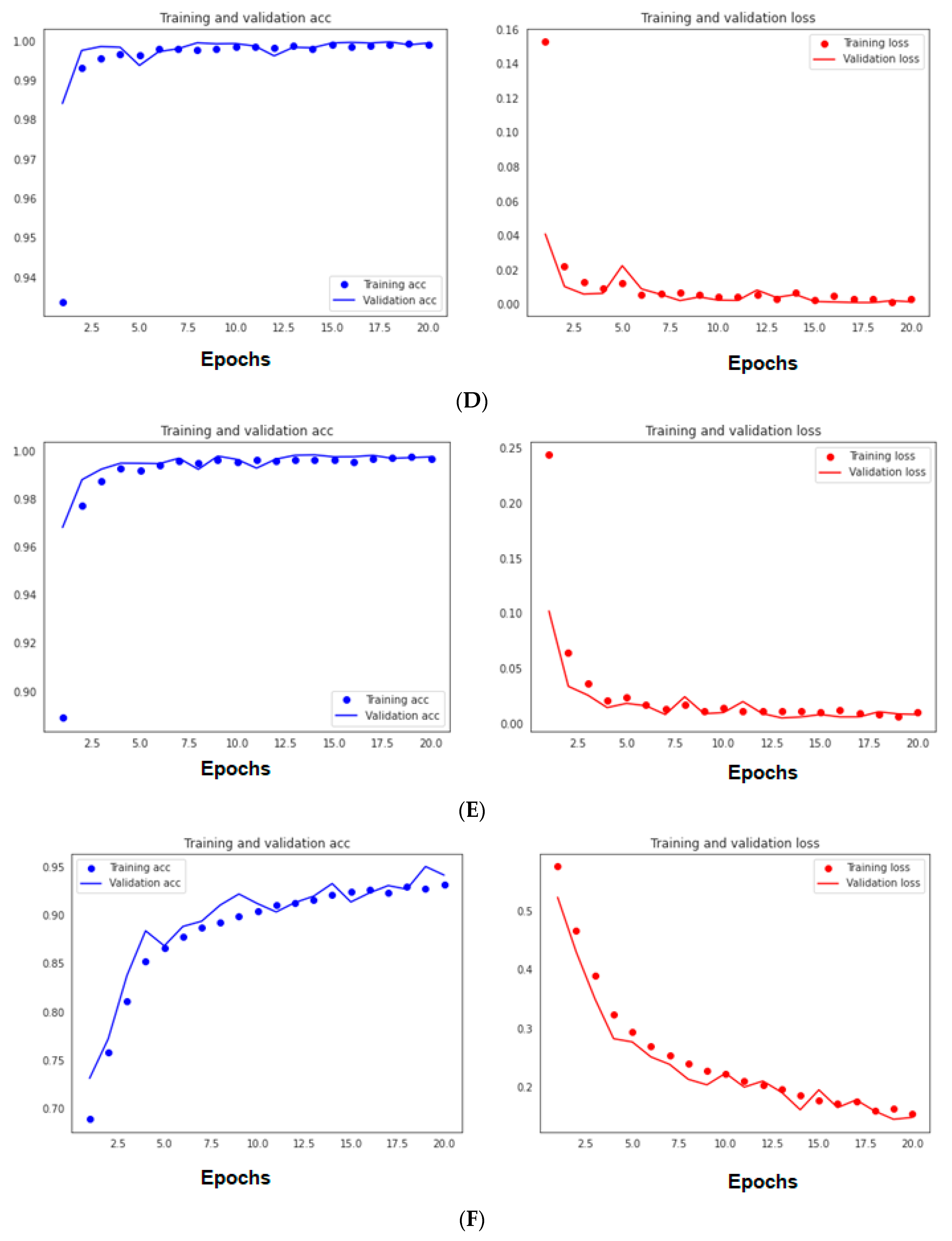
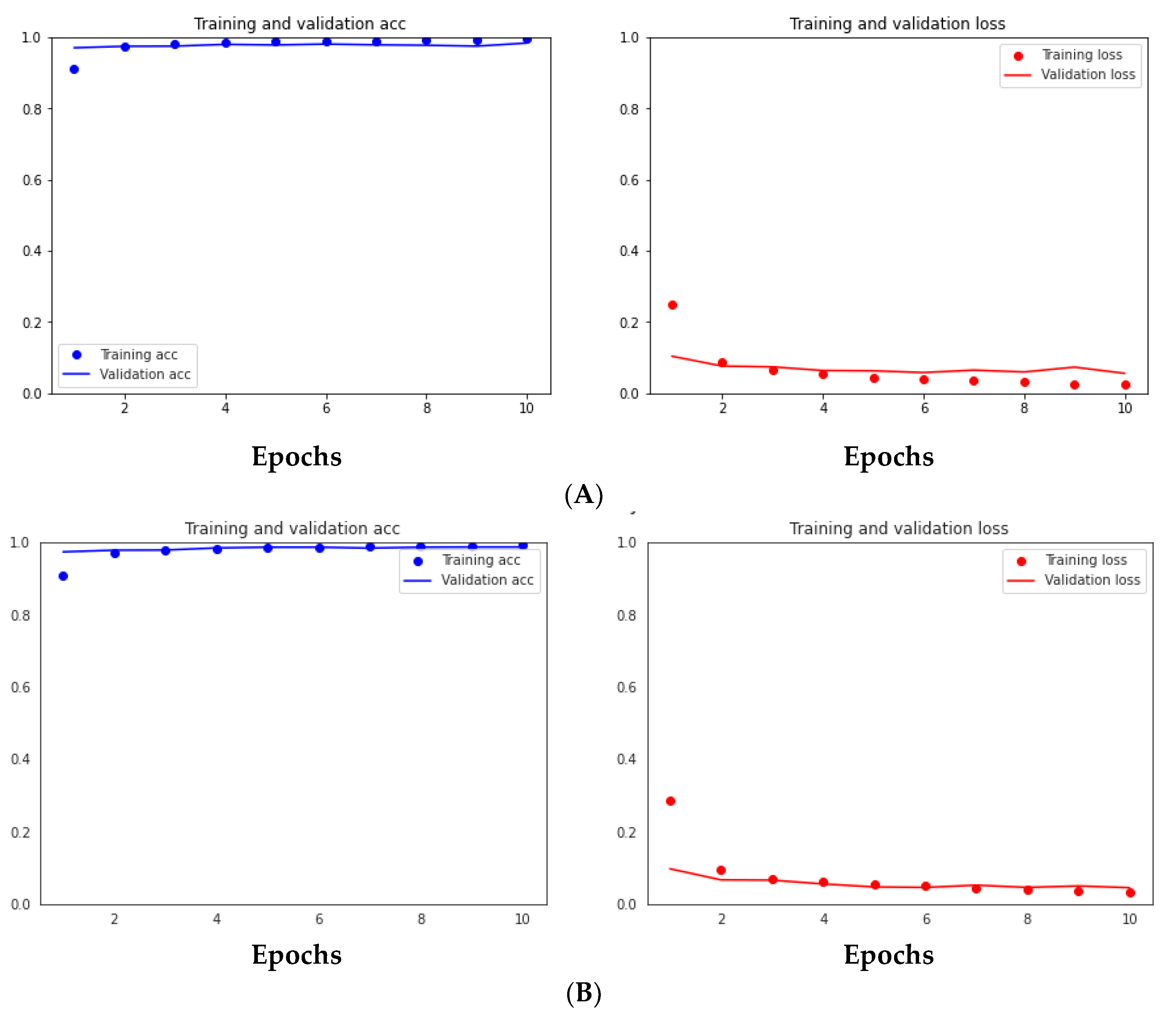
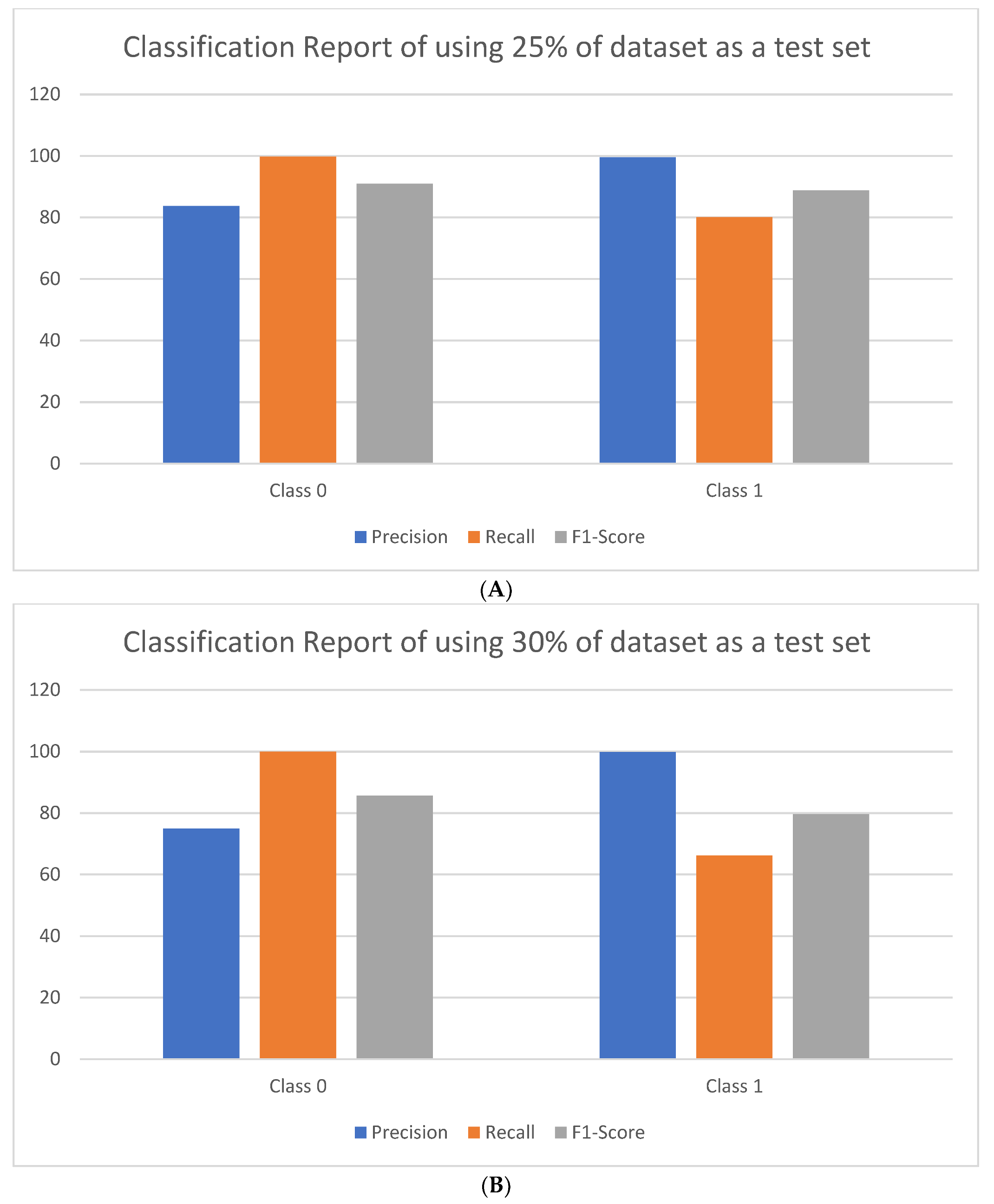
3.5.3. Results of Using Many Split Criteria for Both Malware Datasets

In these scenarios, the split rate of the malware dataset into training and testing will be evaluated. For the first malware dataset, we will use the “12 features-selected” scenario as a basis for three experiments in which the splitting is changed from 20% to 25% and then 30% of the test set, and the results are shown in

Table 6. The split evaluation results of the first six scenarios of the first malware test dataset.

Scenario	V.acc%	T.acc%	Precision %	Recall %	F1-Score%	T.Time (S/Ep)
21 features with 20% for test set	99.75	99.79	99.8	99.8	99.8	2.1
21 features with 25% for test set	99.65	99.62	91.6	89.9	89.9	2.3
21 features with 30% for test set	99.67	99.62	87.5	83.1	82.7	2.1

.

Table 6 shows that increasing the test set percentage will decrease the performance. The main problem of using more test samples appears with the recall of “0-class” samples (the benign samples) and the precision of the “1-class” samples for 25% splitting scenarios, as shown in Figure 6a. The same results are concluded for the 30% split scenario (as shown in Figure 6b). To conclude, the best splitting scenario is using 20% of the test set, and any further increase in test samples will affect either the acceptance rate or the rejection rate (recall and precision).

For the second dataset, the same splitting scenarios will be used based on the “39 features selected” scenario.

Table 7. The evaluation results of the first six scenarios of the second malware test dataset.

Scenario	V.acc%	T.acc%	Precision %	Recall %	F1-Score%	T.Time (S/Ep)
39 features with 20% for test set	94.59	95.34	95.9	94.1	94.9	1.1
39 features with 25% for test set	95.03	94.86	94.9	94	94.4	1.1
39 features with 30% for test set	94.49	94.43	94.3	93.7	94	1.1

illustrates the results of these splitting scenarios.

Changing the splitting criteria of the second dataset shows less performance instability than in the first dataset splitting scenarios. This is due to the different nature of both datasets. The first dataset has a large number of samples with a small number of features, while the second dataset has a small number of samples with a large number of features. The second reason is that the feature selection techniques have different effects on both datasets.

Several feature selection approaches were used in previous studies. Gumaa [37], for example, divided their dataset into three categories based on graph-based feature selection, getting 110 features (51.4%) for permission-only types, 73 features (33.95%) for API calls, and 182 features (85%) for permissions and API calls. Their approach achieved recall values of 95%, 96%, and 97.3%, respectively. In our study, using the same dataset, we applied three different scenarios, getting into 39, 27, and 14 features, respectively (18.22%, 12.61%, and 6.54% of the entire dataset). Our proposed methodology is more effective in selecting the appropriate features of the dataset. Moreover, the recall value of our models using the proposed feature selection approach on the second dataset was 94.1% (very close to the [37] study recall of 95%, although their approach selected more features than our algorithm did).

In the study of Smmarwar et al. [30], the wrapping feature selection (WFS) method was proposed. The study applied the proposed approach to the CIC-InvesAndMal2019 malware dataset. The SVM, RF, and DT models were trained using the selected features and achieved 82.33%, 91.32%, and 91.8% accuracy, respectively.

In a recent publication, Smmarwar et al. [38] used the Binary Grey Wolf Optimization (BGWO)-based meta-heuristic feature selection algorithm to select the best combination of features in a malware dataset. However, the heuristic algorithm takes too much computational time. Our methodology is very easy and takes less than a second to compute the correlations. The study [38] approach is powerful but time-consuming. They achieved accuracies of 70.64%, 65.44%, 59.93%, and 83.49% on the features-selected version of the malware dataset.

A detailed comparison between the current research and previous ones is listed in

Table 8. Comparison between the current research and related work.

Study	Methodology	Dataset	Results
Xiao et al. [39]	LSTM	3536 benign 3567 malware	Acc = 93%
Vinayakumar et al. [3]	KNN, SVM, RF, LR, NB, DNN	70,140 benign and 69,869 malware recodes	Acc = 98.9%
Vinod et al. [40]	RF	100 benign 100 malware records	Acc = 91.7%
Jeon and Moon [25]	CNN encoder and RNN	1000 benign and 1000 malware files	Acc = 96%, Recall = 95%
Yazdinejad et al. [26]	LSTM	200 benign and 500 malware records	Acc = 98%
Darabian et al. [27]	CNN-LSTM	1500 executable samples	Acc = 99%
Hwang et al. [28]	DNN	10,000 malware records and 10,000 benign files	Acc = 94%
Ban et al. [29]	CNN	28,179 records	Acc = 98%, F1-score = 82%
Current study	Dense Model, LSTM model	50,000 malware and 50,000 benign records (35 attributes)	Acc = 99.99%, F1-score = 100% (no feature selection) Acc = 99.75%, F1-score = 99.8% (63.63 selected features)
		9476 benign and 5560 malware records (215 attributes)	Acc = 98.38%, F1-score = 98.9% (no feature selection) Acc = 94.59%, F1-score = 94.9% (18.22% selected features)

, and another detailed comparison between our methodology and previous ML ones that worked on the same dataset is listed in Table 9.

Table 8 shows that the current study’s performance exceeds most other related works’ results. The used dataset size is also larger than most other studies’ datasets. The variety of using two datasets with different specifications and under different feature selection scenarios is also introduced in our study.

Compared to the previous studies, our study used a very large dataset. Other studies used small (Yazdinejad et al. [26], Vinod et al. [40]) or medium datasets (Xiao et al. [39], Jeon and Moon [25], Darabian et al. [27]). Besides that, two different datasets with a variety of features were used in our study to evaluate high dimensionality and big data size.

From a methodology point of view, not only machine learning but also different deep learning models were used in our study. Previous studies applied only one type of ML and DL.

The evaluation process in previous studies used the accuracy metric (Xiao et al. [39], Vinayakumar et al. [3], Vinod et al. [40], Darabian et al. [27], Hwang et al. [28]). Some other studies (Jeon and Moon [25] and Ban et al. [29]) used accuracy, F1-score, and recall. In our study, other metrics like accuracy, F1-score, recall, and precision were also used.

Our study discussion also applied feature selection and different splitting scenarios, which were not taken into account in all previous studies.

Table 9. Comparison between the current research and previous machine learning approaches on the same dataset.

Study	Methodology	Dataset	Results
Taha and Barukab [41]	SVM, logistic regression (LR), gradient boosting (GB), decision tree (DT), and AdaBoost, Ensemble Learning	Second Dataset	Acc= DT: 93.75% LR: 92.86% GB: 93.53% AdaBoost: 90.96% Ensemble Learning: 94.15%
Masum and Shahriar [42]	DT, SVM, LR	Second Dataset	Acc= DT: 97.83% SVM: 97.29% LR: 97.77%
Gumaa [37]	DT, RF, K-NN, LOG	Second Dataset	Acc= RF: 97% LR: 95% DT: 96.5% LOG: 95.5%
Current study	Dense Model, LSTM model	First Dataset	Acc = 99.99%, F1-score = 100% (no feature selection) Acc = 99.75%, F1-score = 99.8% (63.63% selected features)
Current study	Dense Model, LSTM model	Second Dataset	Acc = 98.38%, F1-score = 98.9% (no feature selection) Acc = 94.59%, F1-score = 94.9% (18.22% selected features)

Table 9. Comparison between the current research and previous machine learning approaches on the same dataset.

Study	Methodology	Dataset	Results
Taha and Barukab [41]	SVM, logistic regression (LR), gradient boosting (GB), decision tree (DT), and AdaBoost, Ensemble Learning	Second Dataset	Acc= DT: 93.75% LR: 92.86% GB: 93.53% AdaBoost: 90.96% Ensemble Learning: 94.15%
Masum and Shahriar [42]	DT, SVM, LR	Second Dataset	Acc= DT: 97.83% SVM: 97.29% LR: 97.77%
Gumaa [37]	DT, RF, K-NN, LOG	Second Dataset	Acc= RF: 97% LR: 95% DT: 96.5% LOG: 95.5%
Current study	Dense Model, LSTM model	First Dataset	Acc = 99.99%, F1-score = 100% (no feature selection) Acc = 99.75%, F1-score = 99.8% (63.63% selected features)
Current study	Dense Model, LSTM model	Second Dataset	Acc = 98.38%, F1-score = 98.9% (no feature selection) Acc = 94.59%, F1-score = 94.9% (18.22% selected features)

Table 9 shows that the proposed deep learning LSTM and Dense model exceed the performance of all previous machine learning approaches. The best accuracy score of all previous studies in Table 9 is 97.77% for the logistic regression model (Gumaa study [37]), which is less than our score by 0.61%.

4. Conclusions

In this research, two different malware datasets were used to train and test deep learning models. The first dataset has a large number of records with a low number of attributes. In contrast, the second dataset has a low number of records but a high number of attributes (high dimensionality and complexity). The main purpose of this difference was to evaluate the effect of feature selection on the performance of low- and high-dimensional datasets. For each dataset, many training scenarios were applied. Some of them corresponded with the different selected features, while others were based on various splitting criteria.

The feature selection step was done using the correlation degree between each attribute and the target column (classification column). The most correlated features were selected in 4 different scenarios of the first dataset, starting with dropping six features, nine features, 12 features, and ending with dropping 19 features. With 27 selected features out of 33, the validation accuracy was minimized only by 0.07%, while in the final scenario (with a 42.42% reduction rate), the validation accuracy was reduced by 5.84% and the computational time was also reduced by 0.1 S/Ep.

For the second dataset, the dimension reduction process affected the performance since it has only 15,036 records but 214 attributes (predictors). Another cause of this effect is the high dimensionality of the second dataset, so that the correlation values between the classification column and other columns (predictors) are very close, making a threshold-based feature selection process drop more columns compared to the first dataset (with a small number of columns). The results indicated that by using only 18.22% of the total columns (81.77% reduction rate), the validation accuracy would be reduced by 3.79%, and by using only 6.5% of the total columns, the validation accuracy was reduced by 9.44%. The experiments on both datasets proved that some of the malware dataset’s columns are not actually involved in the final prediction and could be moved out. In the scenarios of the first dataset, the LSTM-added layer enhanced the validation and test accuracies by 0.05% and 0.44%, respectively. The LSTM layer, on the other hand, preserved performance with increased time complexity in the second dataset of scenarios.

Different splitting scenarios were also applied to both datasets. However, in all experiments, the results proved that using 20% as a test set was the best option.

The main limitation of our study was that we focused on the general malware detection task without going deep into the types of malware. In future work, the different malware types can be involved and studied to determine the effect of feature selection on the final prediction of such malware types.

References

1. Rathore, H.; Agarwal, S.; Sahay, S.; Sewak, M. Malware detection using machine learning and deep learning. In Proceedings of the International Conference on Big Data Analytics, Seattle, WA, USA, 10–13 December 2018; pp. 402–411. [Google Scholar]
2. Nasif, A.; Othman, Z.; Sani, N.S. The deep learning solutions on lossless compression methods for alleviating data load on IoT nodes in smart cities. Sensors 2021, 21, 4223. [Google Scholar] [CrossRef] [PubMed]
3. Vinayakumar, R.; Alazab, M.; Soman, K.; Poornachandran, P.; Venkatraman, S. Robust intelligent malware detection using deep learning. IEEE Access 2019, 7, 46717–46738. [Google Scholar] [CrossRef]
4. Singh, A.; Kumar, R. A two-phase load balancing algorithm for cloud environment. Int. J. Softw. Sci. Comput. Intell. 2021, 13, 38–55. [Google Scholar] [CrossRef]
5. Mat, S.R.T.; Razak, M.A.; Kahar, M.; Arif, J.; Firdaus, A. A Bayesian probability model for Android malware detection. ICT Express 2022, 8, 424–431. [Google Scholar] [CrossRef]
6. Yen, S.; Moh, M.; Moh, T.-S. Detecting compromised social network accounts using deep learning for behavior and text analyses. Int. J. Cloud Appl. Comput. 2021, 11, 97–109. [Google Scholar] [CrossRef]
7. Shabudin, S.; Sani, N.; Ariffin, K.; Aliff, M. Feature selection for phishing website classification. Int. J. Adv. Comput. Sci. Appl. 2020, 11, 587–595. [Google Scholar] [CrossRef]
8. Liu, C.-H.; Zhang, Z.-J.; Wang, S.-D. An android malware detection approach using Bayesian inference. In Proceedings of the 2016 IEEE International Conference on Computer and Information Technology (CIT), Nadi, Fiji, 8–10 December 2016; pp. 476–483. [Google Scholar]
9. GDATA Mobile Malware Report—No let-up with Android malware. 2019. Available online: https://www.gdatasoftware.com/news/2019/07/35228-mobile-malware-report-no-let-up-with-android-malware (accessed on 22 November 2022).
10. Qiu, J.; Zhang, J.; Luo, W.; Pan, L.; Nepal, S.; Xiang, Y. A survey of android malware detection with deep neural models. ACM Comput. Surv. 2020, 53, 1–36. [Google Scholar] [CrossRef]
11. Sihwail, R.; Omar, K.; Ariffin, K.A.Z. An effective memory analysis for malware detection and classification. Comput. Mater. Contin. 2021, 67, 2301–2320. [Google Scholar] [CrossRef]
12. Mat, S.R.T.; Razak, M.A.; Kahar, M.; Arif, J.; Mohamad, S.; Firdaus, A. Towards a systematic description of the field using bibliometric analysis: Malware evolution. Scientometrics 2021, 126, 2013–2055. [Google Scholar] [CrossRef]
13. Bassel, A.; Abdulkareem, A.; Alyasseri, Z.; Sani, N.; Mohammed, H.J. Automatic Malignant and Benign Skin Cancer Classification Using a Hybrid Deep Learning Approach. Diagnostics 2022, 12, 2472. [Google Scholar] [CrossRef]
14. Jerlin, M.A.; Marimuthu, K. A new malware detection system using machine learning techniques for API call sequences. J. Appl. Secur. Res. 2018, 13, 45–62. [Google Scholar] [CrossRef]
15. Abdallah, A.; Ishak, M.K.; Sani, N.S.; Khan, I.; Albogamy, F.R.; Amano, H.; Mostafa, S.M. An Optimal Framework for SDN Based on Deep Neural Network. Comput. Mater. Contin. 2022, 73, 1125–1140. [Google Scholar] [CrossRef]
16. Han, H.; Lim, S.; Suh, K.; Park, S.; Cho, S.; Park, M. Enhanced android malware detection: An svm-based machine learning approach. In Proceedings of the 2020 IEEE International Conference on Big Data and Smart Computing (BigComp), Busan, Republic of Korea, 19–22 February 2020; pp. 75–81. [Google Scholar]
17. Singh, P.; Borgohain, S.; Kumar, J. Performance Enhancement of SVM-based ML Malware Detection Model Using Data Preprocessing. In Proceedings of the 2022 2nd International Conference on Emerging Frontiers in Electrical and Electronic Technologies (ICEFEET), Patna, India, 24–25 June 2022; pp. 1–4. [Google Scholar]
18. Droos, A.; Al-Mahadeen, A.; Al-Harasis, T.; Al-Attar, R.; Ababneh, M. Android Malware Detection Using Machine Learning. In Proceedings of the 2022 13th International Conference on Information and Communication Systems (ICICS), Irbid, Jordan, 21–23 June 2022; pp. 36–41. [Google Scholar]
19. Baldini, G.; Geneiatakis, D. A performance evaluation on distance measures in KNN for mobile malware detection. In Proceedings of the 2019 6th international conference on control, decision and information technologies (CoDIT), Paris, France, 23–26 April 2019; pp. 193–198. [Google Scholar]
20. Assegie, T.A. An optimized KNN model for signature-based malware detection. Tsehay Admassu Assegie. Int. J. Comput. Eng. Res. Trends (IJCERT) 2021, 8, 2349–7084. [Google Scholar]
21. Castillo-Zúñiga, I.; Luna-Rosas, F.; Rodríguez-Martínez, L.; Muñoz-Arteaga, J.; López-Veyna, J.; Rodríguez-Díaz, M.A. Internet data analysis methodology for cyberterrorism vocabulary detection, combining techniques of big data analytics, NLP and semantic web. Int. J. Semant. Web Inf. Syst. 2020, 16, 69–86. [Google Scholar] [CrossRef]
22. Yilmaz, A.B.; Taspinar, Y.; Koklu, M. Classification of Malicious Android Applications Using Naive Bayes and Support Vector Machine Algorithms. Int. J. Intell. Syst. Appl. Eng. 2022, 10, 269–274. [Google Scholar]
23. Yildiz, O.; Doğru, I.A. Permission-based android malware detection system using feature selection with genetic algorithm. Int. J. Softw. Eng. Knowl. Eng. 2019, 29, 245–262. [Google Scholar] [CrossRef]
24. Arora, A.; Peddoju, S.; Chouhan, V.; Chaudhary, A. Hybrid Android malware detection by combining supervised and unsupervised learning. In Proceedings of the 24th Annual International Conference on Mobile Computing and Networking, New Delhi, India, 29 October–2 November 2018; pp. 798–800. [Google Scholar]
25. Jeon, S.; Moon, J. Malware-detection method with a convolutional recurrent neural network using opcode sequences. Inf. Sci. 2020, 535, 1–15. [Google Scholar] [CrossRef]
26. Yazdinejad, A.; HaddadPajouh, H.; Dehghantanha, A.; Parizi, R.; Srivastava, G.; Chen, M.-Y. Cryptocurrency malware hunting: A deep recurrent neural network approach. Appl. Soft Comput. 2020, 96, 106630. [Google Scholar] [CrossRef]
27. Darabian, H.; Homayounoot, S.; Dehghantanha, A.; Hashemi, S.; Karimipour, H.; Parizi, R.M.; Choo, K.K.R. Detecting cryptomining malware: A deep learning approach for static and dynamic analysis. J. Grid Comput. 2020, 18, 293–303. [Google Scholar] [CrossRef]
28. Hwang, C.; Hwang, J.; Kwak, J.; Lee, T. Platform-independent malware analysis applicable to windows and linux environments. Electronics 2020, 9, 793. [Google Scholar] [CrossRef]
29. Ban, Y.; Lee, S.; Song, D.; Cho, H.; Yi, J.H. FAM: Featuring Android Malware for Deep Learning-Based Familial Analysis. IEEE Access 2022, 10, 20008–20018. [Google Scholar] [CrossRef]
30. Smmarwar, S.K.; Gupta, G.; Kumar, S. A Hybrid Feature Selection Approach-Based Android Malware Detection Framework Using Machine Learning Techniques. In Cyber Security, Privacy and Networking; Springer: Berlin, Germany, 2022; pp. 347–356. [Google Scholar]
31. Toan, N.N.; Thang, D.Q. Static Feature Selection for IoT Malware Detection. J. Sci. Technol. Inf. Secur. 2022, 1, 74–84. [Google Scholar] [CrossRef]
32. N SARAVANA. Malware Detection|Kaggle. 2018. Available online: https://www.kaggle.com/datasets/nsaravana/malware-detection?select=Malware+dataset.csv (accessed on 22 November 2022).
33. SHASHWAT TIWARI. Android Malware Dataset for Machine Learning|Kaggle. 2018. Available online: https://www.kaggle.com/datasets/shashwatwork/android-malware-dataset-for-machine-learning (accessed on 22 November 2022).
34. Yerima, S.Y.; Sezer, S. Droidfusion: A novel multilevel classifier fusion approach for android malware detection. IEEE Trans. Cybern. 2018, 49, 453–466. [Google Scholar] [CrossRef] [PubMed]
35. Goutte, C.; Gaussier, E. A probabilistic interpretation of precision, recall and F-score, with implication for evaluation. In Proceedings of the European conference on information retrieval, Santiago de Compostela, Spain, 21–23 March 2005; pp. 345–359. [Google Scholar]
36. Van Hulse, J.; Khoshgoftaar, T.; Napolitano, A.; Wald, R. Threshold-based feature selection techniques for high-dimensional bioinformatics data. Netw. Model. Anal. Heal. informatics Bioinforma. 2012, 1, 47–61. [Google Scholar] [CrossRef] [Green Version]
37. Gumaa, M.A. Graph approach for android malware detection using machine learning techniques. Humanit. Nat. Sci. J. 2021, 2, 189–203. [Google Scholar] [CrossRef]
38. Smmarwar, S.K.; Gupta, G.; Kumar, S.; Kumar, P. An optimized and efficient android malware detection framework for future sustainable computing. Sustain. Energy Technol. Assess. 2022, 54, 102852. [Google Scholar] [CrossRef]
39. Xiao, X.; Zhang, S.; Mercaldo, F.; Hu, G.; Sangaiah, A.K. Android malware detection based on system call sequences and LSTM. Multimed. Tools Appl. 2019, 78, 3979–3999. [Google Scholar] [CrossRef]
40. Vinod, P.; Zemmari, A.; Conti, M. A machine learning based approach to detect malicious android apps using discriminant system calls. Futur. Gener. Comput. Syst. 2019, 94, 333–350. [Google Scholar]
41. Taha, A.; Barukab, O. Android Malware Classification Using Optimized Ensemble Learning Based on Genetic Algorithms. Sustainability 2022, 14, 14406. [Google Scholar] [CrossRef]
42. Masum, M.; Shahriar, H. Droid-NNet: Deep learning neural network for android malware detection. In Proceedings of the 2019 IEEE International Conference on Big Data (Big Data), Los Angeles, CA, USA, 9–12 December 2019; pp. 5789–5793. [Google Scholar]
Figure 1. The distribution of Benign (B) and Malware (S) records of the malware dataset.
Symmetry 15 00123 g001
Figure 2. The proposed methodology.
Symmetry 15 00123 g002
Figure 3. Correlation-based feature selection proposed methodology.
Symmetry 15 00123 g003
Figure 4. Training/validation accuracy and loss of the six scenarios of the first dataset: The six scenarios are numbered from (AF).
Symmetry 15 00123 g004aSymmetry 15 00123 g004b
Figure 5. Training/validation accuracy and loss of the six scenarios of the second dataset: the five scenarios are numbered from (AE).
Symmetry 15 00123 g005aSymmetry 15 00123 g005b
Figure 6. Detailed classification report: (A): 25% splitting scenario, (B): 30% splitting scenario.
Symmetry 15 00123 g006