Direct Training via Backpropagation for Ultra-Low-Latency Spiking Neural Networks with Multi-Threshold

Abstract

Spiking neural networks (SNNs) can utilize spatio-temporal information and have the characteristic of energy efficiency, being a good alternative to deep neural networks (DNNs). The event-driven information processing means that SNNs can reduce the expensive computation of DNNs and save a great deal of energy consumption. However, high training and inference latency is a limitation of the development of deeper SNNs. SNNs usually need tens or even hundreds of time steps during the training and inference process, which causes not only an increase in latency but also excessive energy consumption. To overcome this problem, we propose a novel training method based on backpropagation (BP) for ultra-low-latency (1–2 time steps) SNNs with multi-threshold. In order to increase the information capacity of each spike, we introduce the multi-threshold Leaky Integrate and Fired (LIF) model. The experimental results show that our proposed method achieves average accuracy of 99.56%, 93.08%, and 87.90% on MNIST, FashionMNIST, and CIFAR10, respectively, with only two time steps. For the CIFAR10 dataset, our proposed method achieves 1.12% accuracy improvement over the previously reported directly trained SNNs with fewer time steps.

1. Introduction

Spiking neural networks (SNNs) constitute a brain-inspired neural model, which can utilize spatio-temporal information and has an event-driven nature [1,2,3,4]. Unlike traditional artificial neural networks (ANNs), which consist of static and continuous-valued neuron models, SNNs process dynamic and discrete-valued spike events via more biological spiking neuron models [1]. These characteristics mean that SNNs have potential to improve computational and energy efficiency in hardware neuromorphic computing systems [5]. For instance, IBM’s TrueNorth [6] and Intel’s Loihi [7] process a single spike with a few pJ of energy. IMEC proposed a spiking neural network-based chip for radar signal processing that consumes 100 times less power than traditional implementations [8].

However, unlike ANNs, which only need one time forward pass, SNNs usually require multiple time steps of computation to achieve decent performance, resulting in high latency and difficulty to scale up to deeper architectures. Thus, there are two challenges for training an efficient and high-performance SNN. From the algorithmic perspective, the question of how to make full use of rich spatial-temporal information to train SNNs is the greatest challenge of training algorithms. The non-differentiability of discrete spike events makes it difficult to transmit errors precisely. Second, the question of how to minimize the time steps of SNNs without accuracy loss is the key to scaling SNNs to deeper architectures. Fewer time steps, which mean less temporal information that SNNs can utilize, make it difficult to train SNNs with decent performance.

In recent years, many researchers have focused on the problem of the latency of SNNs and tried to solve the problems mentioned above. Some researchers try to propose novel encoding methods to improve the efficiency of information representation to reduce the latency of SNNs [5,9,10,11,12,13]. In [11], the authors proposed an asymmetric gradient weight update method to reduce the training latency, in which the time consumption in Hebbian matrix plastic weight calculations is reduced by performing fewer backpropagation steps by the algorithm. In [13], the authors proposed a phase coding method to encode input spikes by the phase of a global reference clock and achieve latency reduction over the rate coding for image recognition. Compared with rate coding, the proposed method can reduce the number of time steps from hundreds to tens. In [5], the authors proposed a time compression method to compress the temporal domain of spike training, which can achieve up to 16× speedup with little accuracy loss. However, the achievable latency/spike reduction of a particular code can vary widely with the network architecture and application. Furthermore, due to the decrease in the temporal information, the latency of SNNs is difficult to reduce to fewer than ten time steps without accuracy loss by improving the coding methods.

Besides studying various coding methods, there are also some researchers trying to obtain low-latency SNNs from a neuron model and training algorithm perspective [14,15,16]. In [16], the authors proposed a method to obtain the derivative of the postsynaptic potential (PSC) to solve the problem of non-differentiability, enabling the learning of targeted temporal sequences with high timing precision. The proposed method can train a decent-performance SNN in five time steps, but a warm-up mechanism is applied to bring up the firing activity of the network before applying the proposed method, which means that the actual number of time steps is larger than five. In [14], the authors proposed a novel BP-based method that aggregates the finite differences of the loss over multiple perturbed membrane potential waveforms in the neighborhood to compute accurate error gradients. Compared with [16], this training method can achieve a decent-performance SNN in five time steps, without extra steps such as the warm-up mechanism. In [16], an Iterative Initialization and Retraining method for SNNs is proposed in which an ANN is pre-trained and the weights are transmitted to the SNN. The authors explore the feasibility of directly reducing the latency to one time step by modifying the weights and thresholds. Though the proposed method can reduce the latency to one time step, it is still a type of ANN-to-SNN method in which only spatial information is used during the training process. This method neglects the potential of spatio-temporal information, which causes the performance of the converted SNNs to hardly outperform the corresponding ANNs.

In this paper, we propose an architecture of SNN with multi-threshold LIF models, which can transmit and process more information at each time step, and the corresponding direct training method based on the BP algorithm to reduce the latency requirement of SNNs. The main contributions of this article include the following.

(1)

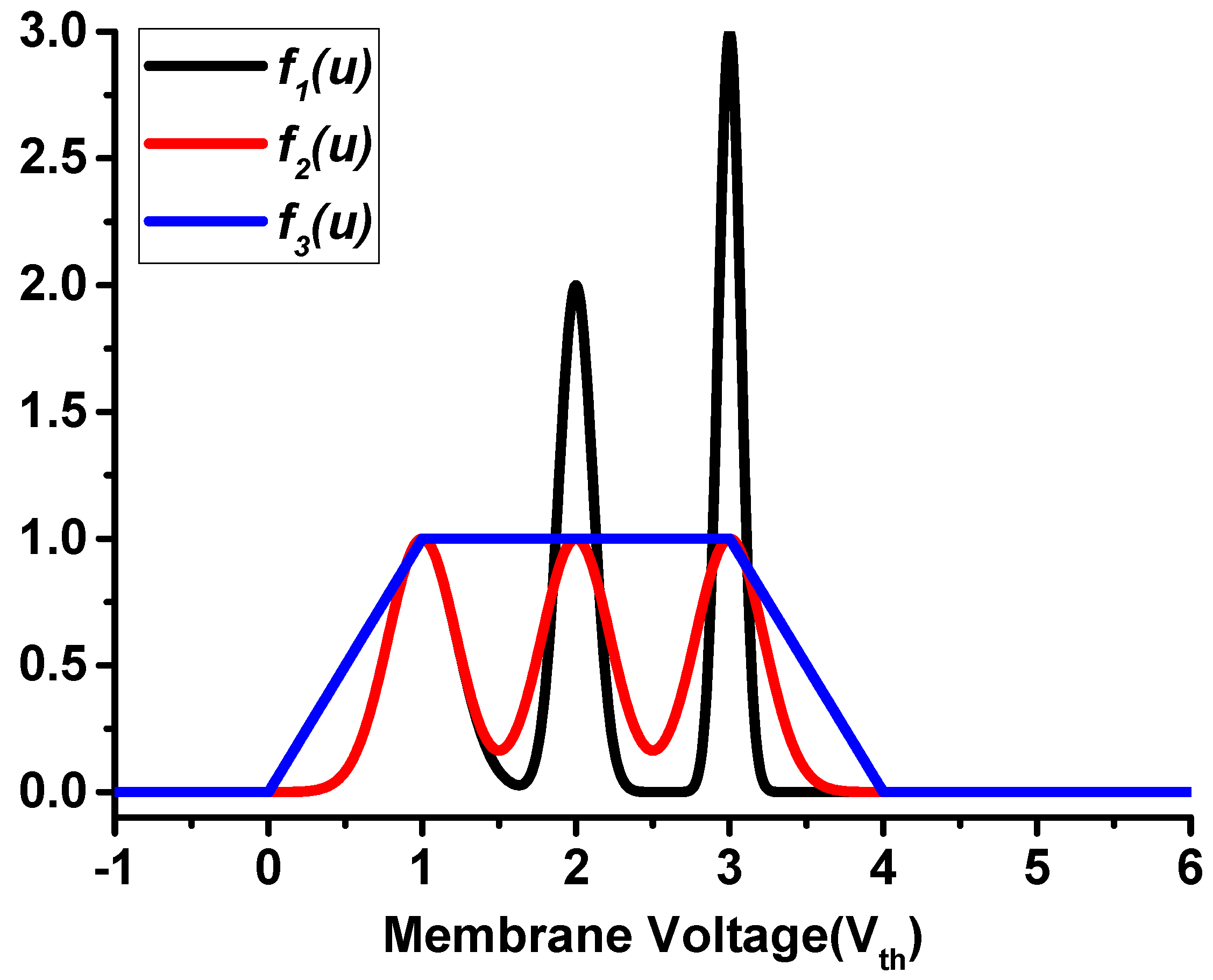
To address the issue of non-differentiability, we propose two axisymmetric surrogate functions and a non-axisymmetric surrogate function to approximate the derivative of spike activity of multi-threshold LIF models.

(2)

Combining the SNN with multi-threshold LIF models and our proposed training algorithm, we can successfully train SNNs at a very short latency, e.g., two time steps.

(3)

We test our SNN framework by using the fully connected and convolution architecture on MNIST [17], FashionMNIST [18], and CIFAR10 [19], and results show that our proposed method achieves an accuracy improvement over the previously reported SNN work with lower latency.

(4)

In addition, we also explore the impact of the symmetry of derivative approximation curves, the number of time steps, etc. This work may help researchers to choose the proper parameters for the method and achieve higher-performance SNNs.

2. Approach

In this section, we introduce our proposed multi-threshold spiking neuron model and the forward pass and the backforward pass of the spiking neural network, which is constructed with multi-threshold LIF models.

2.1. Multi-Threshold Spiking Neuron Model

It is known that the Leaky Integrate and Fire (LIF) model is one of the most widely applied models to describe the neuronal dynamics in SNNs. In this paper, we introduce the LIF neuron model and synaptic model [1] adopted in our work. The neuronal membrane potential of neuron i at time t, $u_i\left(t\right)$, is governed by

$${\tau }_m\frac{d{u}_i\left(t\right)}{dt}=-u_i\left(t\right)+I\left(t\right)+u_{reset}\left(t\right)$$

(1)

where $I\left(t\right)$ is the pre-synaptic input current at time t and ${\tau }_m$ is a time constant of membrane voltage. $u_{reset}\left(t\right)$ denotes the reset function, which reduces the membrane potential by a certain amount $V_{th}$ after the neuron i fires. The pre-synaptic input $I\left(t\right)$ is given by

$$I\left(t\right)=\sum _{j=1}^N{\omega }_{ij}{a}_j\left(t\right)$$

(2)

where N is the number of the pre-synaptic neurons, ${\omega }_{ij}$ is the pre-synaptic weight from the neuron j in the pre-synaptic layer to the neuron i in the post-synaptic layer, $a_j\left(t\right)$ is the synapse response of the pre-synaptic neuron j. In this paper, we apply the zero-th order synaptic model and (2) can be simplified to

$$I\left(t\right)=\sum _{j=1}^N{\omega }_{ij}{s}_j\left(t\right)$$

(3)

where $s_j\left(t\right)$ is the output spike of pre-synaptic neuron j at time t. Due to the discrete time steps in simulation, we apply the fixed-step first-order Euler method to discretize (1) to

$$u_i\left[t\right]=(1-\frac{1}{{\tau }_m})u_i[t-1]+I\left[t\right]+u_{reset}\left[t\right]$$

(4)

where $u_{reset}\left[t\right]$ is equal to $-s_i\left[t\right]V_{th}$ and $s_i\left[t\right]$ is the output spike of neuron i. In this paper, we extend the LIF model into a multi-threshold LIF model, in which the output of the neuron i can be expressed by

$$s_i\left[t\right]=\left\{\begin{array}{cc}\hfill 0,& u_i\left[t\right]<V_{th}\\ \hfill floor\left(\frac{u_i\left[t\right]}{V_{th}}\right),& V_{th}\le u_i\left[t\right]<S_{\mathrm{m}\mathrm{a}\mathrm{x}}{V}_{th}\\ \hfill s_{max},& u_i\left[t\right]\ge S_{\mathrm{m}\mathrm{a}\mathrm{x}}{V}_{th}\end{array}\right.$$

(5)

where $S_{\mathrm{m}\mathrm{a}\mathrm{x}}$ is the upper limit of the output spikes and $floor\left(\right)$ is the function that rounds the elements to the nearest integers towards minus infinity. Figure 1 shows the difference between the LIF model and the multi-threshold LIF model. $s_o\left(t\right)$ is the output of LIF models and $\overline{s_o}\left(t\right)$ is the output of multi-threshold LIF models. When the input spike is sparse, the LIF model and multi-threshold LIF model can transmit the same information by generating output spikes. However, the membrane voltage may reach several times the threshold at one time step, when input spikes are dense.

In this case, the LIF model will drop some information during the information transmission in the network, which may cause the network to require more time steps to compensate for the loss of information. However, as Figure 1b shows, the multi-threshold LIF model can keep the information by introducing a multi-threshold mechanism. Comparing Figure 1a,b, we can see that the multi-threshold LIF model only needs two time steps to obtain a correct classification, but the LIF model cannot make a distinction even in six time steps. In other words, the multi-threshold LIF model has more power information capacity and the network constructed with the multi-threshold LIF model has more potential for low latency.

It should be noticed that the multi-threshold mechanism has no biological representation.

2.2. Proposed Methods

In this subsection, we will introduce the information transmission in the forward pass and the gradient calculation in the backforward pass in detail.

2.2.1. Forward Pass

Without loss of generality, we use two adjacent layers, $l-1$ and l, with $N_{l-1}$ and $N_l$ neurons, respectively, to show the forward pass of a fully connected feed-forward SNN, which is shown in Figure 2. In the forward pass, spike train $s^{(l-1)}\left[t\right]=[s_1^{(l-1)}\left[t\right],\dots ,s_{N_{l-1}}^{(l-1)}\left[t\right]]$ of the $l-1$ layer generates the pre-synaptic input $I^{(l-1)}\left[t\right]=[i_1^{(l-1)}\left[t\right],\dots ,i_{N_{l-1}}^{(l-1)}\left[t\right]]$ by multiplying the corresponding synaptic weight matrix $W^{\left(l\right)}=[{\omega }_1^{\left(l\right)},\dots ,{\omega }_{N_l}^{\left(l\right)}]$, in which ${\omega }_{N_l}^{\left(l\right)}=[{\omega }_{1,N_l}^{\left(l\right)};{\omega }_{2,N_l}^{\left(l\right)};\dots ;{\omega }_{N_{l-1},N_l}^{\left(l\right)}]$. The membrane potentials $u^l\left[t\right]=[u_1^l\left[t\right],\dots ,u_{N_l}^l\left[t\right]]$ update based on (4) and trigger the output spikes of the layer l neurons $s^{\left(l\right)}\left[t\right]=[s_1^{\left(l\right)}\left[t\right],\dots ,s_{N_l}^{\left(l\right)}\left[t\right]]$ based on (5) when the membrane potentials exceed the threshold. We give a concise pseudo-code based on Pytorch for an explicitly iterative multi-threshold LIF model in Algorithm 1.

Algorithm 1: State update for an explicitly iterative multi-threshold LIF neuron at time step t in the l-th layer.

2.2.2. Backforward Pass

In order to present our proposed learning algorithm, we define the following loss function $L\left[t_k\right]$ in which the mean square error for each output neuron at time step $t_k$ is to be minimized

$$L\left[t_k\right]=\frac{1}{2}\sum _{i=0}^{N_o}{(y_i\left[t_k\right]-s_i\left[t_k\right])}^2$$

(6)

where $N_o$ is the number of neurons in the output layer; $y_i\left[t_k\right]$ and $s_i\left[t_k\right]$ denote the desired and the actual firing event of neurons i in the output layer at time step $t_k$.

By combining Equations (1)–(6) together, it can be seen that loss function $L\left[t_k\right]$ is a function of synaptic weight W, which is required for our proposed algorithm based on gradient descent. Figure 3 shows the error propagation in the spatial and temporal domain (STD). The data flow of error propagation in the SD is similar to [20]. Each neuron accumulates the weighted error from the upper layer and updates its parameter using the chain rule. In the TD, the current state of membrane voltage is dependent on its previous state, which makes it complicated to obtain the $\partial L\left[t_k\right]/\partial W$. Equations (7)–(13) show the error calculation process. It should be noticed that the two-sense red arrow in the forward path means that the output spike $s^{\left(l\right)}\left[t_n\right]$ is calculated based on the membrane potential $u^{\left(l\right)}\left[t_n\right]$, and if the neuron is fired, the membrane potential $u^{\left(l\right)}\left[t_n\right]$ will be reset based on the output spike $s^{\left(l\right)}\left[t_n\right]$ in the forward pass process.

The goal of the backforward pass is to update the synaptic weights W using the error gradient $\partial L\left[t_k\right]/\partial W$ at time step $t_k$. Using the chain rule, the error gradient with respect to the pre-synaptic weight $W^{\left(l\right)}$ in the layer l is

$$\frac{\partial L\left[t_k\right]}{\partial W^{\left(l\right)}}=\frac{\partial L\left[t_k\right]}{\partial u^{\left(l\right)}\left[t_k\right]}\frac{\partial u^{\left(l\right)}\left[t_k\right]}{\partial W^{\left(l\right)}}$$

(7)

We use ${\delta }^{\left(l\right)}\left[t_k\right]$ to denote $\partial L\left[t_k\right]/\partial u^{\left(l\right)}\left[t_k\right]$, which is the backpropagated error of layer l at time $t_k$, and (7) can be written as

$$\frac{\partial L\left[t_k\right]}{\partial W^{\left(l\right)}}={\delta }^{\left(l\right)}\left[t_k\right]\frac{\partial u^{\left(l\right)}\left[t_k\right]}{\partial W^{\left(l\right)}}$$

(8)

From (8), the first term ${\delta }^{\left(l\right)}\left[t_k\right]$ can be computed from

$$\begin{array}{c}{\delta }^{\left(l\right)}\left[t_k\right]=\frac{\partial u^{(l+1)}\left[t_k\right]}{\partial u^{\left(l\right)}\left[t_k\right]}\frac{\partial L\left[t_k\right]}{\partial u^{(l+1)}\left[t_k\right]}\hfill \\ =\frac{\partial s^{\left(l\right)}\left[t_k\right]}{\partial u^{\left(l\right)}\left[t_k\right]}\frac{\partial u^{(l+1)}\left[t_k\right]}{\partial s^{\left(l\right)}\left[t_k\right]}{\delta }^{(l+1)}\left[t_k\right]\hfill \\ =\frac{\partial s^{\left(l\right)}\left[t_k\right]}{\partial u^{\left(l\right)}\left[t_k\right]}{\left(W^{(l+1)}\right)}^T{\delta }^{(l+1)}\left[t_k\right]\hfill \end{array}$$

(9)

For the output layer l, (9) can be computed from

$$\begin{array}{c}{\delta }^{\left(l\right)}\left[t_k\right]=\frac{\partial L\left[t_k\right]}{\partial s^{\left(l\right)}\left[t_k\right]}\frac{\partial s^{\left(l\right)}\left[t_k\right]}{\partial u^{\left(l\right)}\left[t_k\right]}\hfill \\ =(s^{\left(l\right)}\left[t_k\right]-y\left[t_k\right])\frac{\partial s^{\left(l\right)}\left[t_k\right]}{\partial u^{\left(l\right)}\left[t_k\right]}\hfill \end{array}$$

(10)

From (4), the second term $\partial u^{\left(l\right)}\left[t_k\right]/\partial W^{\left(l\right)}$ is given by

$$\begin{array}{c}\frac{\partial u^{\left(l\right)}\left[t_k\right]}{\partial W^{\left(l\right)}}=(1-\frac{1}{{\tau }_m})\frac{\partial u^{\left(l\right)}\left[t_{k-1}\right]}{\partial W^{\left(l\right)}}+s^{l-1}\left[t_k\right]-\frac{\partial s^{\left(l\right)}\left[t_k\right]}{\partial W^{\left(l\right)}}{V}_{th}\hfill \\ =(1-\frac{1}{{\tau }_m})\frac{\partial u^{\left(l\right)}\left[t_{k-1}\right]}{\partial W^{\left(l\right)}}+s^{l-1}\left[t_k\right]-\frac{\partial s^{\left(l\right)}\left[t_k\right]}{\partial u^{\left(l\right)}\left[t_k\right]}\frac{\partial u^{\left(l\right)}\left[t_k\right]}{\partial W^{\left(l\right)}}{V}_{th}\hfill \end{array}$$

(11)

Based on (11), we can obtain

$$\frac{\partial u^{\left(l\right)}\left[t_k\right]}{\partial W^{\left(l\right)}}=\frac{(1-\frac{1}{{\tau }_m})\frac{\partial u^{\left(l\right)}\left[t_{k-1}\right]}{\partial W^{\left(l\right)}}+s^{l-1}\left[t_k\right]}{1+\frac{\partial s^{\left(l\right)}\left[t_k\right]}{\partial u^{\left(l\right)}\left[t_k\right]}{V}_{th}}$$

(12)

When $t_{k-1}$ is 0, (12) can be simplified to

$$\frac{\partial u^{\left(l\right)}\left[t_k\right]}{\partial W^{\left(l\right)}}=\frac{s^{l-1}\left[t_k\right]}{1+\frac{\partial s^{\left(l\right)}\left[t_k\right]}{\partial u^{\left(l\right)}\left[t_k\right]}{V}_{th}}$$

(13)

As shown above, for both the output layer and hidden layers, once $\frac{\partial s^{\left(l\right)}\left[t_k\right]}{\partial u^{\left(l\right)}\left[t_k\right]}$ is known, the error can be backpropagated and the gradient of each layer and the update of weights can be calculated.

Theoretically, $s^{\left(l\right)}\left[t\right]$ is a non-differentiable function, which greatly challenges the effective learning of SNNs. Figure 4 shows the multi-step activation function of the spike activity and its original derivative function, which is a set of Dirac functions with infinite value at $u=n{V}_{th},(n>0)$ and zero value at other points. To solve this problem, we introduce three curves to approximate $\frac{\partial s^{\left(l\right)}\left[t_k\right]}{\partial u^{\left(l\right)}\left[t_k\right]}$ by $f_1$, $f_2$, and $f_3$.

$$f_1\left(u\right)=\sum _{i=1}^{s_{max}}i{\alpha }_H{e}^{-{(u-i{V}_{th})}^2/({\alpha }_W/i)}$$

(14)

$$f_2\left(u\right)=\sum _{i=1}^{s_{max}}{\alpha }_H{e}^{-{(u-i{V}_{th})}^2/{\alpha }_W}$$

(15)

$$f_3\left(u\right)=\left\{\begin{array}{cc}\hfill 0,& \hfill u<0\left|\right|u\ge (S_{max}+1)V_{th}\\ \hfill \frac{{\alpha }_{H}u}{V_{th}},& \hfill 0\le u<V_{th}\\ \hfill {\alpha }_H,& \hfill V_{th}\le u<S_{max}{V}_{th}\\ \hfill {\alpha }_H(S_{max}+1-\frac{u}{V_{th}}),& \hfill S_{max}{V}_{th}\le u<(S_{max}+1)V_{th}\end{array}\right.$$

(16)

where ${\alpha }_H$ and ${\alpha }_W$ determine the curve shape and steep degree. $s_{\mathrm{m}\mathrm{a}\mathrm{x}}$ is the upper limit of the output spikes. In Section 3.4, we will compare and analyze the influence on the SNNs’ performance with different curves and different values of parameters, such as ${\alpha }_H$ and $s_{\mathrm{m}\mathrm{a}\mathrm{x}}$. Figure 5 shows the curve of $f_1$, $f_2$, and $f_3$, when $s_{max}$ is 3 and ${\alpha }_H$ and ${\alpha }_W$ are both 1.

3. Experiments and Results

We test our proposed SNN model and training method on three image datasets, MNIST [17], FashionMNIST [18], and CIFAR10 [19], with different sizes and structures of SNNs. Then, we compare our training method with several previously reported state-of-the-art results obtained with the same or similar networks, including different SNNs trained by BP-based methods, converted SNNs, and traditional ANNs.

3.1. Experimental Settings

All reported experiments below are conducted on an NVIDIA Tesla V100 GPU. The implementation of our proposed method is based on the Pytorch framework [21]. The experimented SNNs are based on the multi-threshold LIF model described in (3)–(5). The simulation step size is set to 1 ms. Function $f_2$ is applied to approximate the derivative of spike activity. Only two time steps are used to demonstrate the proposed ultra-low-latency spiking neural network. No refractory period is used. Adam [22] is applied as the optimizer. In this paper, the accuracy is calculated by $AC=RN/n$, where $RN$ is the number of the correctly classified samples, n is the total number of samples, $AC$ = accuracy. If not otherwise specified, the accuracy in this paper refers to the mean of the accuracy obtained by repeating the experiments five times.

3.2. Parameter Initialization

The initialization of parameters, such as the weights, threshold, time constant of membrane voltage, and other parameters, directly affects the convergence speed and stability of the whole network. We should simultaneously ensure that enough spikes transmit information between neural network layers and avoid too many spikes, which could reduce the neuronal selectivity. As it is known that weight and threshold are two key factors for the LIF model in the forward pass [20], in this paper, we use a fixed threshold in each neuron for simplification and initialize the weight $W^{\left(l\right)}$ parameters sampling from the normal distribution.

$$W^{\left(l\right)}\sim [\frac{V_{th}}{N_{l-1}},0.5]$$

(17)

where $V_{th}$ is the threshold of membrane voltage, and $N_{l-1}$ is the number of neurons of pre-layer. The set of other parameters is presented in

Table 1. Parameter settings.

Parameter	Description	Value
${\tau }_m$	Time constant of membrane voltage	10 ms
$V_{th}$	Threshold	10 mV
${\alpha }_m$	Derivative approximation parameters	1
${\alpha }_W$	Derivative approximation parameters	20
$S_{\mathrm{m}\mathrm{a}\mathrm{x}}$	Upper limit of output spikes	15
$N_{Batch}$	Batch size	128
$\eta$	Learning rate (MNIST/FashionMNIST/CIFAR10)	0.005, 0.005, 0.0005
${\beta }_1,{\beta }_2,\lambda$	Adam parameters	0.9, 0.999, $1-{10}^{-8}$

. In addition, we do not apply complex steps, such as error normalization [23], dropout, weight regularization [24], warm-up mechanism [16], etc. In the preprocessing step, the dataset is normalized and only random cropping is applied for data augmentation. All testing accuracy is reported after training 200 epochs in our experiments.

3.3. Dataset Experiments

In this subsection, we compare our method with state-of-the-art methods on the MNIST, FashionMNIST, and CIFAR 10 datasets.

3.3.1. MNIST

The MNIST dataset of handwritten digits [17] consists of a training set with 60,000 labeled hand-written digits, and a test set of 10,000 labeled hand-written digits, each of which is a $28\times 28$ grayscale image. Each pixel value of images is converted into a real-valued input current as in [16]. For the MNIST dataset [17], we compare several similar spiking Multi-Layer Perceptron (MLP) models, each of which consists of one to three hidden layers. The converted SNN applies the ANN-to-SNN method, and STDP [25], BP [24], and STBP [20] all train the spiking neural network by the BP algorithm, directly.

Table 2. Comparison with similar spiking MLP models on MNIST.

Methods	Network	Time Steps	Accuracy
Converted SNN [23] *	784-1200-1200-10	20	98.64%
STDP [25]	784-6400-10	350	95.00%
BP [24]	784-800-10	200-1000	98.71%
STBP [20]	784-800-10	50-300	98.89%
Proposed Method	784-800-10	2	99.15%

* means that their model is converted from the pre-trained ANN model.

shows that the spiking MLP trained by our method can achieve $99.15\%$, which outperforms other reported results and obtains a large reduction in time step count. Moreover, we also compare several spiking Convolutional Neural Networks (CNNs), each of which consists of two convolutional layers, two pooling layers, and a fully connected layer. Table 2 shows that the spiking MLP trained by our method can achieve $99.15\%$, which outperforms other reported results and obtains a large reduction in time step count. SLAYER [26], HM2BP [27], ST-RSBP [28], and TSSL-BP [16] all use BP algorithms to train the spiking neural network, directly.

Table 3. Comparison with similar spiking CNNs on MNIST.

Methods	Network	Time Steps	Accuracy
SLAYER [26]	12C5-P2-64C5-p2 1	300	99.36%
HM2BP [27]	15C5-P2-40C5-P2-300	400	99.42%
ST-RSBP [28]	15C5-P2-40C5-P2-300	400	99.57%
TSSL-BP [16]	15C5-P2-40C5-P2-300	5	99.47%
Proposed Method	15C5-P2-40C5-P2-300	2	99.56%

¹ 12C5 represents convolution layer with 12 of the 5 × 5 filters; P2 represents pooling layer with 2 × 2 filters; 300 means fully connected layers with 300 neurons.

shows the test accuracies of the spiking CNNs trained by our proposed method and other reported algorithms, except for the method in [28], whose accuracy is only slightly higher by $0.01\%$. However, our proposed method obtains up to $99.56\%$ in only two time steps, which is much fewer than the 400 time steps that [28] needs.

3.3.2. FashionMNIST

The FashionMNIST dataset of clothing items contains 60,000 labeled training images and 10,000 labeled testing images, each of which is also a $28\times 28$ grayscale image, as with MNIST. Compared with MNIST, FashionMNIST is a more challenging dataset that can serve as a direct drop-in replacement for the original MNIST dataset. We compare trained spiking MLPs and CNNs on FashionMNIST. In

Table 4. Comparison with spiking MLPs on FashionMNIST.

Methods	Network	Time Steps	Accuracy
ANN [28] *	784-512-512-10		89.01%
HM2BP [27]	784-400-400-10	400	88.99%
ST-RSBP [28]	784-400-400-10	400	90.13%
TSSL-BP [16]	784-400-400-10	5	90.19%
Proposed Method	784-400-400-10	2	91.08%

* means that their model is the non-spiking ANN trained by a standard BP method.

, ANN [28] is the non-spiking ANN trained by a standard BP method. HM2BP [27], ST-RSBP [28], and TSSL-BP [16] use BP algorithms to train the spiking neural network, directly. We compare our proposed method with other methods on the same architecture of two hidden layers. Our proposed method obtains $91.08\%$ test accuracy, outperforming the TSSL-BP method [16], which is the best previously reported algorithm for SNNs, as far as we know. In addition, compared with [16], our method reduces the training time steps from 5 to 2, further.

Table 5. Comparison with spiking CNNs on FashionMNIST.

Methods	Network	Time Steps	Accuracy
ANN *1	32C5-P2-64C5-P2-1024		91.60%
TSSL-BP [16]	32C5-P2-64C5-P2-1024	5	92.45%
Converted SNN *2	16C5-P2-64C5-P2-1024	200	92.62%
Proposed Method	32C5-P2-64C5-P2-1024	2	93.08%

*¹ means that their model is the non-spiking ANN trained by a standard BP method; *² means that their model is converted from the pre-trained ANN model.

compares CNNs with similar architectures. Our method achieves $93.08\%$ in two time steps, which shows that it outperforms other methods and reduces the training time steps noticeably.

3.3.3. CIFAR10

To validate our method, we apply a deeper CNN that contains five convolutional layers, two pooling layers, and two fully connected layers on the more challenging dataset of CIFAR10 [19]. Different from MNIST and FashionMNIST, CIFAR10 is a subset of 80 million tiny images and consists of 60,000 32 × 32 color images containing one of 10 object classes, with 6000 images per class. In addition, it is difficult to scale to deeper networks for traditional SNNs, which need long training latency. To the best of our knowledge, only a few works report the direct training of SNNs on CIFAR10, which we list in

Table 6. Comparison with spiking CNNs on CIFAR10.

Methods	Skills	Time Steps	Accuracy
ANN [29] *1	Random cropping		83.72%
Converted SNN [29] *2	Random cropping		83.52%
STBP [30]	Neuron normalization, dropout, and population decoding	8	85.24%
TSSL-BP [16]	Random cropping and horizontal flipping	5	86.78%
Proposed Method	Random cropping	2	87.90%

*¹ means that their model is the non-spiking ANN trained by a standard BP method; *² means that their model is converted from the pre-trained ANN model. The network structure is 96C3-256C3-P2-384C3-P2-384C3-256C3-1024-1024.

. Our proposed method obtains $88.17\%$ accuracy with a mean of $87.90\%$. Compared with TSSL-BP [16], our method achieves $1.12\%$ average testing accuracy improvement with fewer time steps and fewer additional optimization and augmentation technologies.

3.4. Performance Analysis

In this subsection, we analyze the impact of derivative approximation curves, the impact of $S_{\mathrm{m}\mathrm{a}\mathrm{x}}$, and the impact of the length of the spiking train.

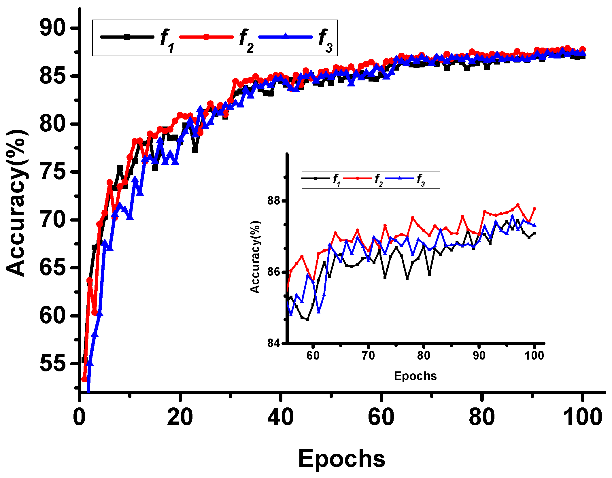
3.4.1. The Impact of Derivative Approximation Curves

In Section 2.2.2, we introduce two axisymmetric surrogate functions and a non-axisymmetric surrogate function to approximate the spike activity. In this section, we try to make a comparison and analyze the impact of the symmetry of curves on the performance of the trained network. The experiments are conducted on the CIFAR10 dataset, and the network structure is 96C3-256C3-P2-384C3-P2-384C3-256C3-1024-1024, which is the same as described in Section 3.3.3. The parameter of curves is the same as in Table 1. As Figure 6 shows, the three curves present similar performance. For curve 1, the value of the curve may be larger than 1 when the membrane voltage is larger than the two thresholds, which may cause gradient exploding problems in deep networks. For curves 2 and 3, the symmetry of the functions maintains a reasonable approximation of the network gradient and ensures that the values of curves will not be larger than 1, which avoids the gradient exploding problem. Compared with curve 3, curve 2 gives a more reasonable approximation and shows a slight improvement. Thus, we choose curve 2 to approximate the spike activity in this paper.

Furthermore, we choose curve 2 to explore the impact of the parameters of curves. The main parameters of the derivative approximation curves are ${\alpha }_W$ and ${\alpha }_H$. Due to the gradient exploding problem mentioned above, we fix the value of ${\alpha }_H$ to 1 and focus on the impact of different widths of the curve, which is controlled by ${\alpha }_W$. ${\alpha }_W$ is set to 0.2, 2, 20, 200, 2000, and two time steps are applied in the experiments. The corresponding testing accuracy after 100 epochs is shown in Figure 7. A small ${\alpha }_W$ will cause worse performance. When ${\alpha }_W$ is larger than 20, the testing accuracy has a slight decrease. The reason that the shape of the derivative approximation curves is not very sensitive to the accuracy is that the main function of these curves is to capture the nonlinear nature [20].

3.4.2. The Impact of S_Max

$S_{\mathrm{m}\mathrm{a}\mathrm{x}}$ is the upper limit of the output spikes, which directly affects the capacity of information at each time step. In this section, we study the impact of $S_{\mathrm{m}\mathrm{a}\mathrm{x}}$ on the accuracy. Curve 2 is applied and the same experiment configuration is set. To shield the influence of the temporal domain, the training time step is set to 1. As Figure 8 shows, the network still achieves reasonable accuracy even when only one time step is applied, if the $S_{\mathrm{m}\mathrm{a}\mathrm{x}}$ is large enough for spikes to have enough information capacity. The testing accuracy reaches $87.82\%$ when $S_{\mathrm{m}\mathrm{a}\mathrm{x}}$ is 15. Moreover, the testing accuracy will be saturated when $S_{\mathrm{m}\mathrm{a}\mathrm{x}}$ is larger than 7. As we know that SNNs can utilize the information of the temporal domain and spatial domain, the information of each spike can be treated as spatial domain information and the positions of spikes in the spike train carry temporal information. When the value of $S_{\mathrm{m}\mathrm{a}\mathrm{x}}$ allows a spike to have enough capacity for information to transmit all spatial information in the SNN, the increase in $S_{\mathrm{m}\mathrm{a}\mathrm{x}}$ will not improve the accuracy.

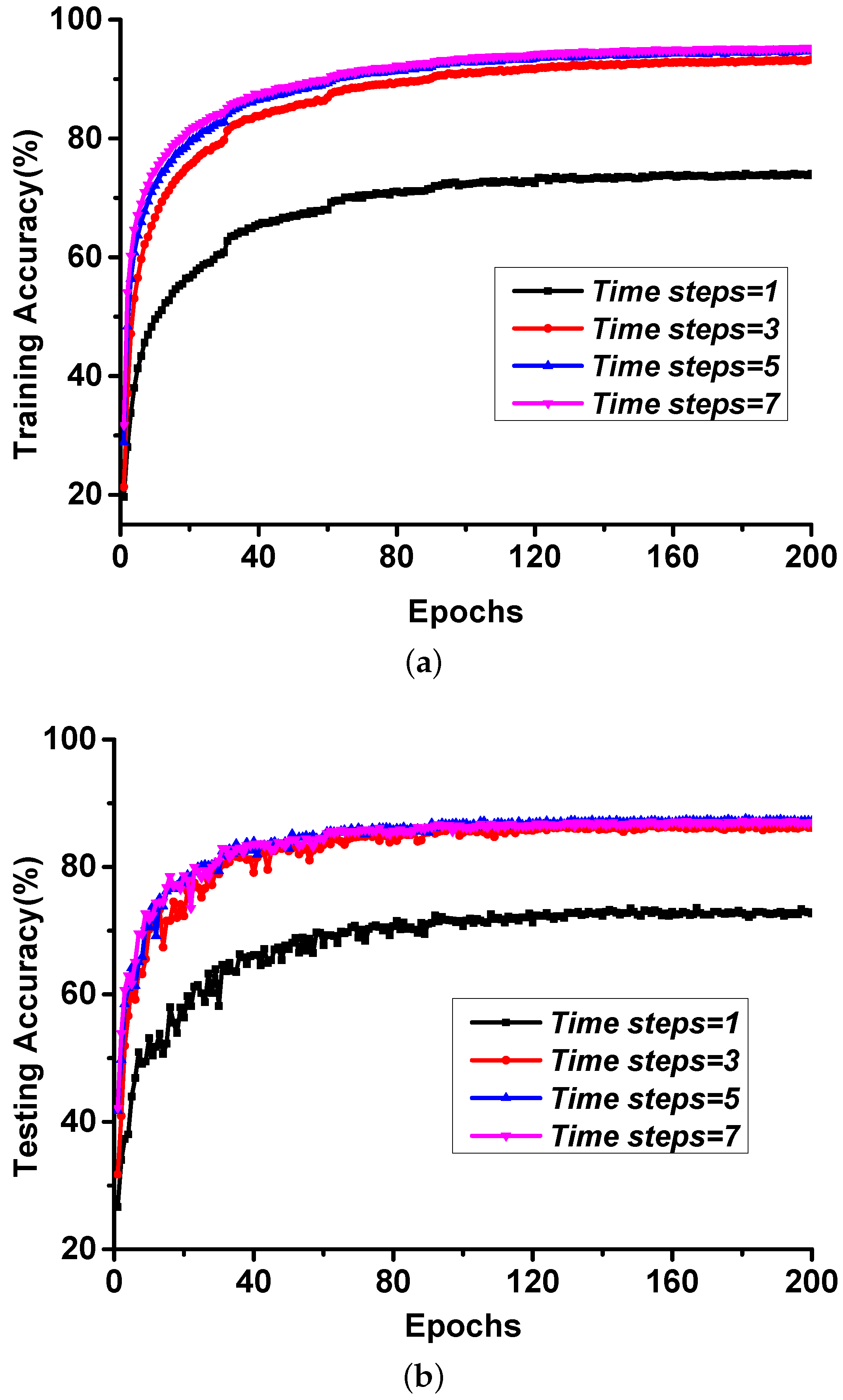
3.4.3. The Impact of Length of Spike Train

For SNNs, a longer spike train may carry more temporal information, theoretically. In this section, we mainly study the impact of the length of spike trains on performance. Curve 2, whose $S_{\mathrm{m}\mathrm{a}\mathrm{x}}$ is 1, is applied and the same experiment configuration is set. The number of time steps is used to measure the length of spike trains. Figure 9 shows the testing and training accuracy for different time steps. Compared with the SNN with one time step, which contains no temporal information, the SNN with multi-time steps can improve the performance of the SNN. Compared with the SNN with one time step, the SNN with five time steps improves the testing accuracy from $73.60\%$ to $87.55\%$. As Figure 9 shows, the testing accuracy is no longer improved when the number of time steps is larger than 3. However, the training accuracy is still improved with the increase in the time steps. The reason for this is that the increase in the length of spike trains improves the capacity for temporal information, which can improve the performance. However, temporal information is very sensitive, which may reduce the robustness of the trained networks. An overly long spike train may cause network overfitting if other training techniques are not applied.

4. Conclusions and Future Work

In this paper, we presented a novel training method based on backpropagation for ultra-low-latency spiking neural networks. The LIF model with multi-threshold is introduced to enable the SNN to carry more spatial information in each time step. We also proposed three approximated derivative curves to address the non-differentiable problem of multi-threshold spike activity and proposed a training method based on backpropagation. We demonstrated the state-of-the-art performance in comparison with the SNN BP method, converted SNNs, and even traditional ANNs on the MNIST, FashionMNIST, and CIFAR10 datasets. Experimental results showed that our proposed method outperformed other SNN BP methods with the same or similar network architecture, regardless of accuracy and latency. In short, we tried to propose a method to address the high training and inference latency issue of SNNs and present the possibility of training an SNN with ultra-low latency directly.

In this paper, we merely tried to modify the LIF model to improve its information capacity by introducing a multi-threshold mechanism. In the future, we will explore an efficient information transmission mechanism in biological organisms to propose a biologically inspired mechanism to improve the efficiency of information transmission in spiking neural networks.

References

1. Gerstner, W.; Kistler, W.M. Spiking Neuron Models: Single Neurons, Populations, Plasticity; Cambridge University Press: Cambridge, UK, 2002. [Google Scholar]
2. Xiang, S.; Jiang, S.; Liu, X.; Zhang, T.; Yu, L. Spiking vgg7: Deep convolutional spiking neural network with direct training for object recognition. Electronics 2022, 11, 2097. [Google Scholar] [CrossRef]
3. Zhong, X.; Pan, H. A spike neural network model for lateral suppression of spike-timing-dependent plasticity with adaptive threshold. Appl. Sci. 2022, 12, 5980. [Google Scholar] [CrossRef]
4. Dora, S.; Kasabov, N. Spiking neural networks for computational intelligence: An overview. Big Data Cogn. Comput. 2021, 5, 67. [Google Scholar] [CrossRef]
5. Xu, C.; Zhang, W.; Liu, Y.; Li, P. Boosting throughput and efficiency of hardware spiking neural accelerators using time compression supporting multiple spike codes. Front. Neurosci. 2020, 14, 104. [Google Scholar] [CrossRef] [PubMed]
6. Merolla, P.A.; Arthur, J.V.; Alvarez-Icaza, R.; Cassidy, A.S.; Sawada, J.; Akopyan, F.; Jackson, B.L.; Imam, N.; Guo, C.; Nakamura, Y.; et al. A million spiking-neuron integrated circuit with a scalable communication network and interface. Science 2014, 345, 668–673. [Google Scholar] [CrossRef]
7. Davies, M.; Srinivasa, N.; Lin, T.H.; Chinya, G.; Joshi, P.; Lines, A.; Wild, A.; Wang, H. Loihi: A neuromorphic manycore processor with on-chip learning. IEEE Micro. 2018, 38, 82–99. [Google Scholar] [CrossRef]
8. Imec Builds World’s First Spiking Neural Network-Based Chip for Radar Signal Processing. Available online: https://www.imec-int.com/en/articles/imec-builds-world-s-first-spiking-neural-network-based-chip-for-radar-signal-processing (accessed on 31 October 2021).
9. Thorpe, S.; Delorme, A.; Rullen, R.V. Spike-based strategies for rapid processing. Neural Netw. 2001, 14, 715–725. [Google Scholar] [CrossRef]
10. Kayser, C.; Montemurro, M.A.; Logothetis, N.K.; Panzeri, S. Spike-phase coding boosts and stabilizes information carried by spatial and temporal spike patterns. Neuron 2009, 61, 597–608. [Google Scholar] [CrossRef]
11. Magotra, A.; Kim, J. Neuromodulated dopamine plastic networks for heterogeneous transfer learning with hebbian principle. Symmetry 2021, 13, 1344. [Google Scholar] [CrossRef]
12. Alhmoud, L.; Nawafleh, Q.; Merrji, W. Three-phase feeder load balancing based optimized neural network using smart meters. Symmetry 2021, 13, 2195. [Google Scholar] [CrossRef]
13. Jaehyun, K.; Heesu, K.; Subin, H.; Jinho, L.; Kiyoung, C. Deep neural networks with weighted spikes. Neurocomputing 2018, 311, 373–386. [Google Scholar]
14. Chowdhury, S.S.; Rathi, N.; Roy, K. One timestep is all you need: Training spiking neural networks with ultra low latency. arXiv 2021, arXiv:2110.05929. [Google Scholar]
15. Yang, Y.; Zhang, W.; Li, P. Backpropagated neighborhood aggregation for accurate training of spiking neural networks. In Proceedings of the 38th International Conference on Machine Learning (ICML2021), Virtual, 18–24 July 2021. [Google Scholar]
16. Zhang, W.; Li, P. Temporal spike sequence learning via backpropagation for deep spiking neural networks. arXiv 2020, arXiv:2002.10085. [Google Scholar]
17. Lecun, Y.; Bottou, L. Gradient-based learning applied to document recognition. Proc. IEEE 1998, 86, 2278–2324. [Google Scholar] [CrossRef]
18. Xiao, H.; Rasul, K.; Vollgraf, R. Fashion-mnist: A novel image dataset for benchmarking machine learning algorithms. arXiv 2017, arXiv:1708.07747. [Google Scholar]
19. Krizhevsky, A.; Nair, V.; Hinton, G. The Cifar-10 Dataset. 2014. Available online: http://www.cs.toronto.edu/kriz/cifar.html (accessed on 1 September 2022).
20. Wu, Y.; Lei, D.; Li, G.; Zhu, J.; Shi, L. Spatio-temporal backpropagation for training high-performance spiking neural networks. Front. Neurosci. 2018, 12, 331. [Google Scholar] [CrossRef]
21. Paszke, A.; Gross, S.; Massa, F.; Lerer, A.; Chintala, S. Pytorch: An imperative style, high-performance deep learning library. Adv. Neural Inf. Process. Syst. 2019, 32. [Google Scholar]
22. Kingma, D.P.; Ba, J. Adam: A method for stochastic optimization. arXiv 2014, arXiv:1412.6980. [Google Scholar]
23. Diehl, P.U.; Neil, D.; Binas, J.; Cook, M.; Liu, S.-C.; Pfeiffer, M. Fast-classifying, high-accuracy spiking deep networks through weight and threshold balancing. In Proceedings of the 2015 International Joint Conference on Neural Networks (IJCNN), Killarney, Ireland, 12–17 July 2015; pp. 1–8. [Google Scholar]
24. Lee, J.H.; Delbruck, T.; Pfeiffer, M. Training deep spiking neural networks using backpropagation. Front. Neurosci. 2016, 10, 508. [Google Scholar] [CrossRef]
25. Diehl, P.U.; Cook, M. Unsupervised learning of digit recognition using spike-timing-dependent plasticity. Front. Comput. Neurosci. 2015, 9, 99. [Google Scholar] [CrossRef]
26. Sengupta, A.; Ye, Y.; Wang, R.; Liu, C.; Roy, K. Going deeper in spiking neural networks: Vgg and residual architectures. Front. Neurosci. 2019, 13, 95. [Google Scholar] [CrossRef] [PubMed] [Green Version]
27. Jin, Y.; Zhang, W.; Li, P. Hybrid macro/micro level backpropagation for training deep spiking neural networks. Adv. Neural Inf. Process. Syst. 2018, 31. [Google Scholar]
28. Zhang, W.; Li, P. Spike-train level backpropagation for training deep recurrent spiking neural networks. Adv. Neural Inf. Process. Syst. 2019, 32. [Google Scholar]
29. Hunsberger, E.; Eliasmith, C. Training spiking deep networks for neuromorphic hardware. arXiv 2016, arXiv:1611.05141. [Google Scholar]
30. Wu, Y.; Deng, L.; Li, G.; Zhu, J.; Shi, L. Direct training for spiking neural networks: Faster, larger, better. In Proceedings of the AAAI Conference on Artificial Intelligence, Honolulu, HI, USA, 27 January–1 February 2019; Volume 33, pp. 1311–1318. [Google Scholar]
Figure 1. Illustration of discrete LIF model and multi-threshold LIF model: (a) sparse spiking input, (b) dense spiking input.
Symmetry 14 01933 g001
Figure 2. Forward pass of SNN.
Symmetry 14 01933 g002
Figure 3. Error propagation in the STD.
Symmetry 14 01933 g003
Figure 4. Multi-step activation function of the spike activity and its original derivative function.
Symmetry 14 01933 g004
Figure 5. Three curves to approximate the derivative of spike activity.
Symmetry 14 01933 g005
Figure 6. Comparison of different derivation approximation curves.
Symmetry 14 01933 g006
Figure 7. Impact of different widths of derivation approximation curves.
Symmetry 14 01933 g007
Figure 8. Impact of S m a x on testing accuracy.
Symmetry 14 01933 g008
Figure 9. Impact of the length of time steps: (a) training accuracy, (b) testing accuracy.
Symmetry 14 01933 g009