MLTSP: New 3D Framework, Based on the Multilayer Tensor Spectrum Pyramid

Abstract

A tensor representation structure based on the multilayer tensor spectrum pyramid (MLTSP) is introduced in this work. The structure is “truncated”, i.e., part of the high-frequency spectrum coefficients is cut-off, and on the retained low-frequency coefficients, obtained at the output of each pyramid layer, a hierarchical tensor SVD (HTSVD) is applied. This ensures a high concentration of the input tensor energy into a small number of decomposition components of the tensors obtained at the coder output. The implementation of this idea is based on a symmetrical coder/decoder. An example structure for a cubical tensor of size 8 × 8 × 8, which is represented as a two-layer tensor spectrum pyramid, where 3D frequency-ordered fast Walsh–Hadamard transform and HTSVD are used, is given in this paper. The analysis of the needed mathematical operations proved the low computational complexity of the new approach, due to a lack of iterative calculations. The high flexibility of the structure in respect to the number of pyramid layers, the kind of used orthogonal transforms, the number of retained spectrum coefficients, and HTSVD components, permits us to achieve the desired accuracy of the restored output tensor, imposed by the application. Furthermore, this paper presents one possible application for 3D object searches in a tensor database. In this case, to obtain the invariant representation of the 3D objects, in the spectrum pyramid, the 3D modified Mellin–Fourier transform is embedded, and the corresponding algorithm is shown.

1. Introduction

Processing, storage, transfer, and analysis of multidimensional (MD) images, mathematically represented as MD tensors, recently became a question of particular focus studied in numerous research works. In the last years, various tensor decomposition methods have been developed [1,2,3,4], among which are the multilinear extensions of the matrix SVD, and the generalizations of the SVD matrix for higher-order tensors, called higher-order SVD (HOSVD). This includes several well-known methods: canonical polyadic decomposition (CPD) also known as parallel factor analysis (PARAFAC), where the tensor is represented as a sum of rank-one tensors; the hierarchical Tucker decomposition (H-Tucker), which is a higher-order form of the principal component analysis (PCA); the multilinear PCA (MPCA) [5]; the non-negative tensor factorization (NTF) [6]; the tensor-train decomposition (TTD) [7], etc. For the tensor decomposition components calculation, different iterative methods are used: the alternating least square (ALS) [8]; the tensor power iteration; the higher-order eigenvalue decomposition; the Jacobi algorithm; the QR factorization [9], etc.

Additionally, for object detection in tensor multispectral images, mathematical models of stochastic random fields for the background description are suggested [10]. In this work, the existing contemporary approaches for object detection is based on convolutional neural network (CNN) deep learning with structures of the kind region-based CNN (R-CNN), fast R-CNN, YOLO (You Only Live Once), EfficientDet (efficient object detection), SSD (single-shot detector), etc., which are compared with the introduced new approach, and it is indicated that neural networks ensure high efficiency of object detection, but unlike the approach based on the stochastic random fields models, they demand significant computational resources and a huge amount of priori visual information about the objects.

Tensors play, nowadays, the leading part in modern deep learning architectures. As is known, deep neural networks sometimes perform in an extremely complicated regime, manipulating tens of millions of parameters—much larger than the training data amount. Unlike this, the use of tensor decompositions in deep learning architectures results in a significant reduction in the number of unknown parameters [11].

To achieve computational complexity reduction, a new non-iterative approach for MD tensor image representation based on the multilayer tensor spectrum pyramid (MLTSP) [12] with embedded 3D orthogonal transforms (3D OTs) and hierarchical tensor SVD (HTSVD) [13] is proposed in this work. This approach is illustrated by an example representation of a tensor of the size 8 × 8 × 8 through two-layer tensor spectrum pyramid (2LTSP), with embedded 3D frequency-ordered fast Walsh–Hadamard transform (3D FO-FWHT) [14] and HTSVD for a tensor of the size 2 × 2 × 2 (HTSVD_2×2×2) [13]. Furthermore, one application of the presented pyramidal structure aimed at the accelerated search of 3D objects represented through MLTSP and 3D modified Mellin–Fourier Transform (3D MMFT), which is an upgrade from the previous research of the authors [15], is given in this work.

In the next sections of the paper, more details are given about the new approach; i.e., Section 2 contains the basic relations, which represent the two-layer tensor spectrum pyramid implementation for a tensor of the size 8 × 8 × 8; in Section 3, the HTSVD decomposition algorithm for a spectrum tensor of the size 2 × 2 × 2 (which is the building element in the introduced pyramidal structure) is given; in Section 4, the fast algorithm for 3D FO-FWHT calculation is explained; Section 5 evaluates the computational complexity of 3D-FWHT; in Section 6, the general algorithm for 3D object search in a database of 3D objects represented through MLTSP is given; in Section 7, the invariant 3D object representation based on the 3D MMFT is given; and Section 8 contains the Conclusion.

2. Basic Relations, Which Represent the Two-Layer Tensor Spectrum Pyramid with 3D OT and HTSVD

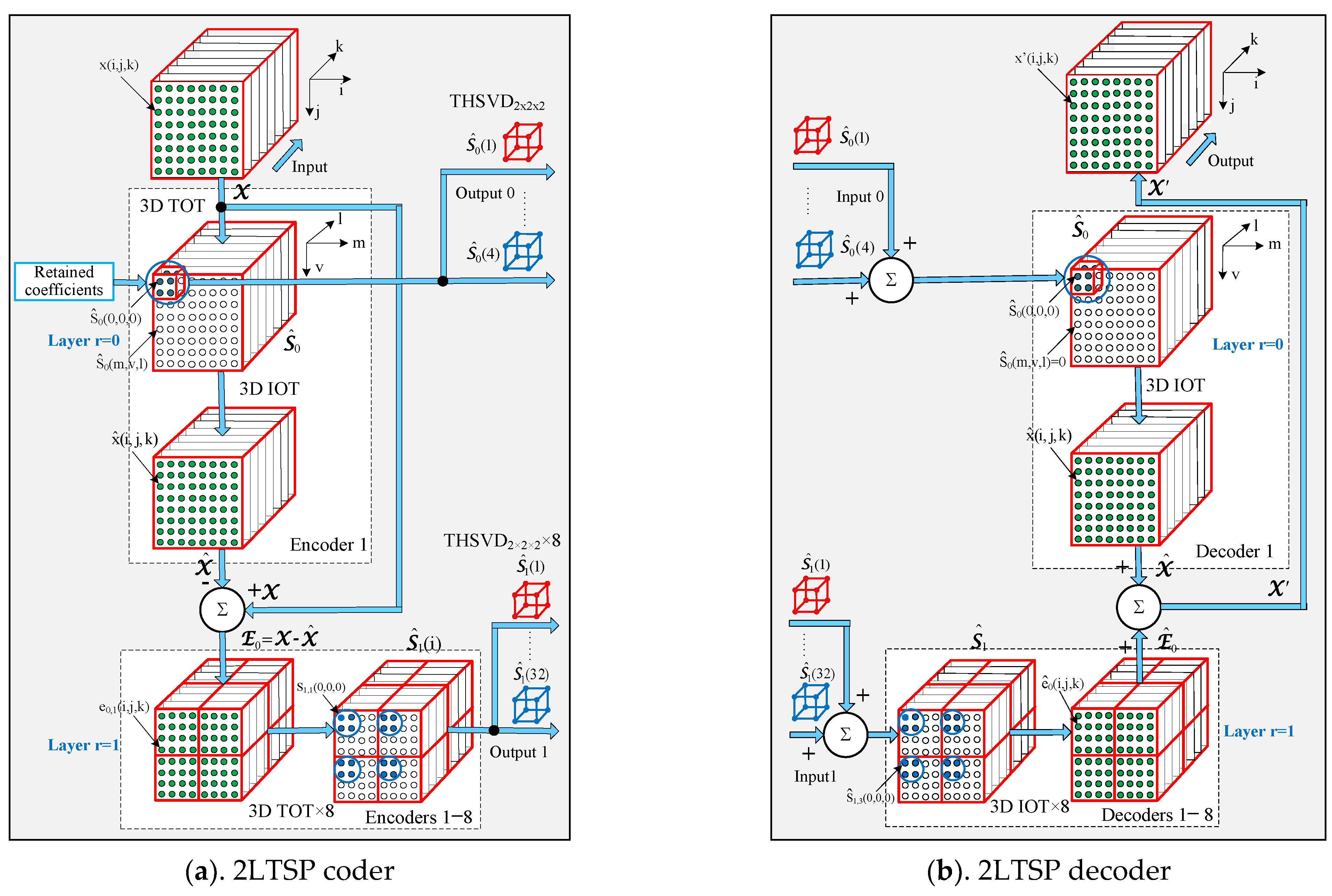
To explain the structure of the multilayer TSP, we use, as an example, the 2LTSP, which comprises a coder and decoder. The structure of the decoder is mirror-symmetrical to that of the coder. The corresponding block diagrams are shown in Figure 1a,b.

The following symbols are used: X—cubical tensor of size N = 2ⁿ for N = 8; r = 0, 1—the 2LTSP layer number; S—cubical spectrum tensor of size N = 2ⁿ; F(.)—operator for direct 3D orthogonal transform (3D OT) (for example, one of the following: 3D FFT [16], 3D FO-AHKLT [17], 3D FO-FWHT [14], etc.); F_T(.)—operator for direct truncated orthogonal transform (3D TOT); F⁻¹(.)—operator for 3D inverse orthogonal transform (3D IOT); HTSVD_2×2×2—hierarchical tensor singular value decomposition for a 2 × 2 × 2 elementary tensor [13].

2.1. Description of the 2LTSP Coder Performance

The performance of the coder (Figure 1a) is presented through the following operations:

In the first layer, for r = 0:

$${\widehat{\mathbf{S}}}_0\hspace{0.17em}={\mathrm{F}}_{\mathrm{T}}(\mathbf{X})$$

(1)

$${\widehat{\mathbf{S}}}_{0,2\times 2\times 2}={\widehat{\mathbf{S}}}_{0,2\times 2\times 2}(1)+{\widehat{\mathbf{S}}}_{0,2\times 2\times 2}(2)+{\widehat{\mathbf{S}}}_{0,2\times 2\times 2}(3)+{\widehat{\mathbf{S}}}_{0,2\times 2\times 2}(4)={\displaystyle \sum _{\mathrm{t}=1}^4{\widehat{\mathbf{S}}}_{0,2\times 2\times 2}(\mathrm{t})}$$

(2)

$$\widehat{\mathbf{X}}\hspace{0.17em}={\mathrm{F}}^{-1}({\widehat{\mathbf{S}}}_0), {\mathbf{E}}_0\hspace{0.17em}=\mathbf{X}\hspace{0.17em}-\hspace{0.17em}\widehat{\mathbf{X}}$$

(3)

Here, ${\widehat{\mathbf{S}}}_0$ denotes the spectrum tensor, which is the approximation of X in the layer r = 0; ${\mathbf{E}}_0$—the difference tensor in the layer r = 0; ${\widehat{\mathbf{S}}}_{0,2\times 2\times 2}$—the spectrum sub-tensor of the size 2 × 2 × 2 in the layer r = 0, which comprises eight low-frequency spectrum coefficients of the selected 3D truncated orthogonal transform (3D TOT); $\widehat{\mathbf{X}}$—the approximation of tensor X; ${\widehat{\mathbf{S}}}_{0,2\times 2\times 2}(\mathrm{t})$—the SVD component t for the sub-tensor ${\widehat{\mathbf{S}}}_{0,2\times 2\times 2}$.

In the second layer, for r = 1:

$${\widehat{\mathbf{S}}}_1(\mathrm{u})={\mathrm{F}}_{\mathrm{T}}\{{\mathbf{E}}_0(\mathrm{u})\} \mathrm{for} \mathrm{u}=1, 2, ..., 8;$$

(4)

$$\begin{gathered} {\widehat{\mathbf{S}}}_{1,2\times 2\times 2}(\mathrm{u})={\widehat{\mathbf{S}}}_{1,2\times 2\times 2}(\mathrm{u},1)+{\widehat{\mathbf{S}}}_{1,2\times 2\times 2}(\mathrm{u},2)+{\widehat{\mathbf{S}}}_{1,2\times 2\times 2}(\mathrm{u},3)+{\widehat{\mathbf{S}}}_{1,2\times 2\times 2}(\mathrm{u},4)={\displaystyle \sum _{\mathrm{t}=1}^4{\widehat{\mathbf{S}}}_{1,2\times 2\times 2}(\mathrm{u},\mathrm{t})}, \\ \text{for}u=1,2,\dots ,8, \end{gathered}$$

(5)

where ${\mathbf{E}}_0(\mathrm{u})$ denotes the u^th difference sub-tensor of the size 4 × 4 × 4; ${\widehat{\mathbf{S}}}_1(\mathrm{u})$—the u^th spectrum sub-tensor of the size 4 × 4 × 4, which is the approximation of the sub-tensor ${\mathbf{S}}_1(\mathrm{u})$ in the layer r = 1; ${\widehat{\mathbf{S}}}_{1,2\times 2\times 2}(\mathrm{u})$—the u^th spectrum sub-tensor of the size 2 × 2 × 2 in the layer r = 1, which comprises eight low-frequency spectrum coefficients of the selected 3D TOT; ${\widehat{\mathbf{S}}}_{1,2\times 2\times 2}(\mathrm{u},\mathrm{t})$—the SVD component t of the sub-tensor ${\widehat{\mathbf{S}}}_{1,2\times 2\times 2}(\mathrm{u})$. At the coder output in the layer r = 0 and in correspondence with Equation (2), four HTSVD_2×2×2 components are obtained, arranged following the decreasing values of their dispersions. At the coder output in the layer r = 1, 32 components of HTSVD_2×2×2 are obtained, calculated in correspondence with Equation (5) for the sub-tensors u = 1, 2, …, 8, and arranged following the decreasing values of their dispersions.

2.2. Description of the 2LTSP Decoder Performance

Because of the mirror symmetry existing in the coder/decoder structures (Figure 1), the performance of the decoder is presented through operations, inverse to these in the coder.

In the first layer, for r = 0:

$${\widehat{\mathbf{S}}}_{0,2\times 2\times 2}={\displaystyle \sum _{\mathrm{t}=1}^4{\widehat{\mathbf{S}}}_{0,2\times 2\times 2}(\mathrm{t})}, {\widehat{\mathbf{S}}}_0={\displaystyle \underset{\mathrm{t}=1}{\overset{4}{\cup }}{\widehat{\mathbf{S}}}_{0,2\times 2\times 2}(\mathrm{t})}$$

(6)

$$\widehat{\mathbf{X}}\hspace{0.17em}={\mathrm{F}}^{-1}({\widehat{\mathbf{S}}}_0)$$

(7)

In accordance with Equation (6), the tensor ${\widehat{\mathbf{S}}}_0$ is restored by uniting the sub-tensors ${\widehat{\mathbf{S}}}_{0,2\times 2\times 2}(\mathrm{t})$ in correspondence with Figure 1b, and the values of the remaining spectrum coefficients (${\widehat{\mathbf{S}}}_0$ voxels) are replaced by zeros.

In the second layer, for r = 1:

$${\widehat{\mathbf{S}}}_{1,2\times 2\times 2}(\mathrm{u})={\displaystyle \sum _{\mathrm{t}=1}^4{\widehat{\mathbf{S}}}_{1,2\times 2\times 2}(\mathrm{u},\mathrm{t})} \text{for} \mathrm{u}=1, 2, ..., 8;$$

(8)

$${\widehat{\mathbf{S}}}_1={\displaystyle \underset{\mathrm{u}=1}{\overset{8}{\cup }}{\displaystyle \underset{\mathrm{t}=1}{\overset{4}{\cup }}{\widehat{\mathbf{S}}}_{1,2\times 2\times 2}(\mathrm{u},\mathrm{t})}}, {\widehat{\mathbf{E}}}_0\hspace{0.17em}={\mathrm{F}}^{-1}({\widehat{\mathbf{S}}}_1)$$

(9)

$${\mathbf{X}}^{\prime }={\widehat{\mathbf{E}}}_0\hspace{0.17em}+\hspace{0.17em}\widehat{\mathbf{X}}.$$

(10)

In accordance with Equation (9), the tensor ${\widehat{\mathbf{S}}}_1$ is restored through uniting the sub-tensors ${\widehat{\mathbf{S}}}_{1,2\times 2\times 2}(\mathrm{u},\mathrm{t})$ in correspondence with Figure 1b, and the values of the remaining spectrum coefficients (voxels of ${\widehat{\mathbf{S}}}_1$) are replaced by zeros. In cases that in the process of 2LTSP coder performance is used, 3D OT instead of 3D TOT, at the output of the decoder 2LTSP, the restored tensor X is obtained, i.e., the transform of the input tensor X through 2LTSP is reversible.

The difference between the original and restored tensors defines the error tensor, ΔX:

$$\Delta \mathbf{X}=\mathbf{X}-{\mathbf{X}}^{\prime }=\mathbf{X}-({\widehat{\mathbf{E}}}_0\hspace{0.17em}+\hspace{0.17em}\widehat{\mathbf{X}}).$$

(11)

The restoration accuracy of the tensor ${\mathbf{X}}^{\prime }$ depends on:

(1)

The number of retained low-frequency spectrum coefficients, which compose the cubical spectrum tensors ${\widehat{\mathbf{S}}}_{0,2\times 2\times 2}$ and ${\widehat{\mathbf{S}}}_{1,2\times 2\times 2}(\mathrm{u})$ for u = 1, 2, …, 8 (in the last case, each spectrum tensor comprises eight coefficients);

(2)

The number of retained components of each HTSVD_2×2×2, applied on the spectrum tensors ${\widehat{\mathbf{S}}}_{0,2\times 2\times 2}$ and ${\widehat{\mathbf{S}}}_{1,2\times 2\times 2}(\mathrm{u})$.

The restoration accuracy of tensor ${\mathbf{X}}^{\prime }$ increases together with the number of retained HTSVD spectrum coefficients, and the use of 3D FO-AHKLT as a basis for 2LTSP. The presented approach could be easily generalized for MTSP of more than two layers. The increase in the number of layers results in a lower power of the error tensor, ΔX.

3. HTSVD Algorithm for Spectrum Tensor Decomposition

In this case, on each tensor S_2×2×2, obtained at the outputs 0 and 1 of the 2LTSP coder shown in Figure 1a, HTSVD_2×2×2 is applied. As a result, a sum of four components is obtained, for which the energy of each tensor is concentrated mainly in the first and second components. This permits us to reduce (cut off) the number of low-energy components without lessening the quality of the restored tensor, in correspondence with Figure 1b.

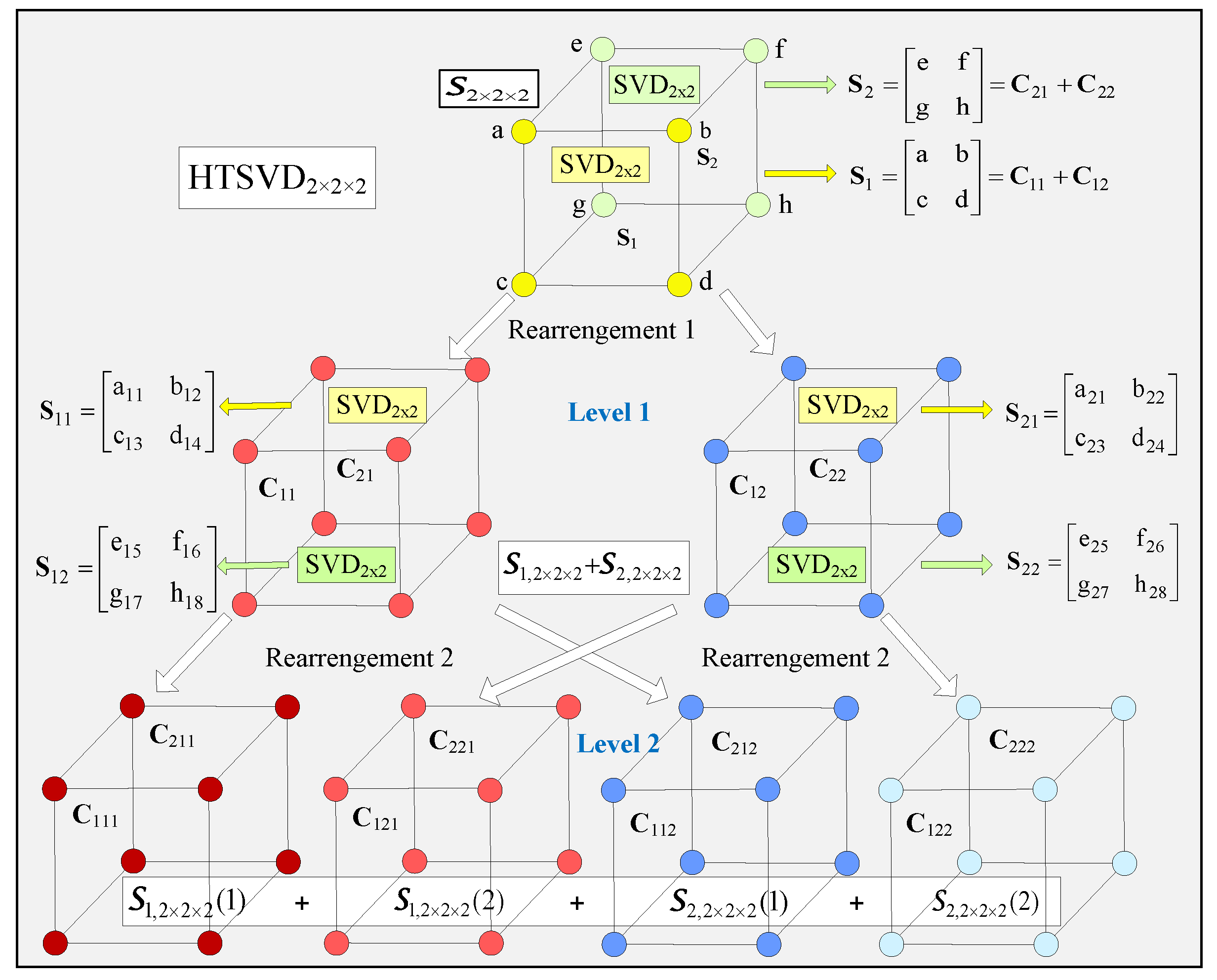
The block diagram of the computational graph of the two-level HTSVD_2×2×2 algorithm for decomposition of the elementary tensor S_2×2×2 is shown in Figure 2. The decomposition is based on SVD for the matrix X of size 2 × 2, denoted as SVD_2×2, and described by the relation below [13]:

$$\mathbf{X}=\left[\begin{array}{cc}\mathrm{a}& \mathrm{b}\\ \mathrm{c}& \mathrm{d}\end{array}\right]\hspace{0.17em}=\frac{1}{2\mathrm{A}}\left\{{\mathsf{\sigma }}_1\left[\begin{array}{cc}\sqrt{\mathrm{r}\mathrm{p}}& \sqrt{\mathrm{s}\mathrm{p}}\\ \sqrt{\mathrm{r}\mathrm{q}}& \sqrt{\mathrm{s}\mathrm{q}}\end{array}\right]+{\mathsf{\sigma }}_2\hspace{0.17em}\left[\begin{array}{cc}\sqrt{\mathrm{s}\mathrm{q}}& -\sqrt{\mathrm{r}\mathrm{q}}\\ -\sqrt{\mathrm{s}\mathrm{p}}& \sqrt{\mathrm{r}\mathrm{p}}\end{array}\right]\hspace{0.17em}\right\}\hspace{0.17em}={\sigma }_1{\mathrm{U}}_1{V}_1^{\mathrm{t}}+{\sigma }_1{\mathrm{U}}_2{V}_2^{\mathrm{t}}\hspace{0.17em}=C_1+C_2\hspace{0.17em}$$

(12)

where a, b, c, and d are the elements of the matrix X, $\mathrm{A}=\sqrt{{\mathsf{\nu }}^2+4{\mathsf{\eta }}^2}\ne 0$, ${\mathsf{\sigma }}_1=\sqrt{\frac{\mathsf{\omega }+\mathrm{A}}{2}}$, ${\mathsf{\sigma }}_2=\sqrt{\frac{\mathsf{\omega }\hspace{0.33em}-\mathrm{A}}{2}}$, ${\mathrm{U}}_1=\frac{1}{\sqrt{2\mathrm{A}}}\left[\begin{array}{c}\sqrt{\mathrm{p}}\\ \sqrt{\mathrm{q}}\end{array}\right]$, ${\mathrm{U}}_2=\frac{1}{\sqrt{2\mathrm{A}}}\left[\begin{array}{c}-\sqrt{\mathrm{q}}\\ \hspace{0.17em}\sqrt{\mathrm{p}}\end{array}\right]$, $V_1=\frac{1}{\sqrt{2\mathrm{A}}}\left[\begin{array}{c}\sqrt{\mathrm{r}}\\ \sqrt{\mathrm{s}}\end{array}\right]$, $V_2=\frac{1}{\sqrt{2\mathrm{A}}}\left[\begin{array}{c}-\sqrt{s}\\ \hspace{0.17em}\sqrt{\mathrm{r}}\end{array}\right]$, $\mathrm{r}=\mathrm{A}+\mathsf{\nu },$$\mathrm{p}=\hspace{0.17em}\mathrm{A}+\mathsf{\mu },$$\mathrm{s}=\mathrm{A}-\mathsf{\nu },$$\mathrm{q}=\hspace{0.17em}\mathrm{A}-\mathsf{\mu },$$\mathsf{\nu }={\mathrm{a}}^2+{\mathrm{c}}^2-{\mathrm{b}}^2-{\mathrm{d}}^2,$$\mathsf{\eta }=\mathrm{a}\mathrm{b}+\mathrm{c}\mathrm{d},$ $\mathsf{\mu }={\mathrm{a}}^2+{\mathrm{b}}^2-{\mathrm{c}}^2-{\mathrm{d}}^2,$ $\mathsf{\omega }={\mathbf{a}}^2+{\mathbf{b}}^2+{\mathbf{c}}^2+{\mathbf{d}}^2$. Since ${\mathsf{\sigma }}_1>>{\mathsf{\sigma }}_2$, the energy of the first decomposition component in (12) is much larger than that of the second. The number of parameters which define SVD_2×2 is four ($\mathsf{\nu },$$\mathsf{\eta },$$\mathsf{\mu },$$\mathsf{\omega }$), i.e., the decomposition is not “over-complete”.

After mode1 unfolding (matricization) of the elementary tensor S_2×2×2, the following is obtained:

$$\mathrm{u}\mathrm{n}\mathrm{f}\mathrm{o}\mathrm{l}\mathrm{d}({\mathbf{S}}_{2\times 2\times 2})=\hspace{0.17em}\left[\begin{array}{cccc}\mathrm{a}& \mathrm{b}& \mathrm{e}& \mathrm{f}\\ \mathrm{c}& \mathrm{d}& \mathrm{g}& \mathrm{h}\end{array}\right]=\left[\begin{array}{cc}\hspace{0.17em}{\mathbf{S}}_1& {\mathbf{S}}_2\end{array}\right]$$

(13)

In the first level of the algorithm HTSVD for the tensor S_2×2×2 (HTSVD_2×2×2), for each matrix S₁ and S₂, an SVD of the size 2 × 2 (SVD_2×2) is executed, and as a result we obtain:

$${\mathbf{S}}_1=\left[\begin{array}{cc}\mathrm{a}& \mathrm{b}\\ \mathrm{c}& \mathrm{d}\end{array}\right]=C_{11}+C_{12},{\mathbf{S}}_2=\left[\begin{array}{cc}\mathrm{e}& \mathrm{f}\\ \mathrm{g}& \mathrm{h}\end{array}\right]=C_{21}+C_{22}$$

(14)

The matrices C_i,j of the size 2 × 2 for i, j = 1, 2, calculated in accordance with Equation (12), are rearranged into new couples in correspondence with their singular values. After this, the first couple of matrices, C₁₁ and C₂₁, which have high singular values, define the tensor S_1(2×2×2) by inverse matricization, and for the second couple, C₁₂ and C₂₂, which have lower singular values, the corresponding tensor is S_2(2×2×2). Then:

$${\mathbf{S}}_{2\times 2\times 2}={\mathbf{S}}_{1(2\times 2\times 2)}+{\mathbf{S}}_{2(2\times 2\times 2)}.$$

(15)

After mode-3 unfolding of both tensors, the following is obtained:

$$\mathrm{u}\mathrm{n}\mathrm{f}\mathrm{o}\mathrm{l}\mathrm{d}\hspace{0.17em}({\mathbf{S}}_{1(2\times 2\times 2)})\hspace{0.17em}+\mathrm{u}\mathrm{n}\mathrm{f}\mathrm{o}\mathrm{l}\mathrm{d}\hspace{0.17em}({\mathbf{S}}_{2(2\times 2\times 2)})=\hspace{0.17em}\left[\begin{array}{cc}\hspace{0.17em}{\mathbf{S}}_{11}& {\mathbf{S}}_{21}\end{array}\right]+\left[\begin{array}{cc}\hspace{0.17em}{\mathbf{S}}_{12}& {\mathbf{S}}_{22}\end{array}\right].$$

(16)

In the second HTSVD_2×2×2 level, SVD_2×2 is applied for each matrix S_i,j of the size 2 × 2, and this result is obtained:

$${\mathbf{S}}_{11}=C_{111}+C_{112},{\mathbf{S}}_{21}=C_{211}+C_{212},{\mathbf{S}}_{12}=C_{121}+C_{122}, {\mathbf{S}}_{22}=C_{221}+C_{222}.$$

(17)

The matrices C_i,j,k of the size 2 × 2 for i, j, k = 1, 2 are rearranged into four new couples, following the decrease in their singular values. After inverse matricization, each of these four couples of matrices defines a corresponding tensor of size 2 × 2 × 2.

In result of the mode1, unfolding is obtained:

$$\begin{array}{c}\mathrm{u}\mathrm{n}\mathrm{f}\mathrm{o}\mathrm{l}\mathrm{d}\{{\mathbf{S}}_{1(2\times 2\times 2)}(1)\}+\mathrm{u}\mathrm{n}\mathrm{f}\mathrm{o}\mathrm{l}\mathrm{d}\{{\mathbf{S}}_{1(2\times 2\times 2)}(2)\}+\mathrm{u}\mathrm{n}\mathrm{f}\mathrm{o}\mathrm{l}\mathrm{d}\{{\mathbf{S}}_{2(2\times 2\times 2)}(1)\}+\mathrm{u}\mathrm{n}\mathrm{f}\mathrm{o}\mathrm{l}\mathrm{d}\{{\mathbf{S}}_{2(2\times 2\times 2)}(2)\}\hspace{0.33em}=\hspace{0.17em}\hfill \\ \left[C_{111}{C}_{211}\hspace{0.17em}\right]+\left[\hspace{0.17em}{C}_{121}{C}_{221}\hspace{0.17em}\right]+\left[\hspace{0.17em}{C}_{112}{C}_{212}\hspace{0.17em}\right]+\hspace{0.17em}\left[C_{122}{C}_{222}\hspace{0.17em}\right].\hfill \end{array}$$

(18)

After execution of the two HTSVD_2×2×2 levels, the tensor ${\mathbf{S}}_{2\times 2\times 2}$ is represented as:

$${\mathbf{S}}_{2\times 2\times 2}={\mathbf{S}}_{1(2\times 2\times 2)}(1)+{\mathbf{S}}_{1(2\times 2\times 2)}(2)+{\mathbf{S}}_{2(2\times 2\times 2)}(1)+{\mathbf{S}}_{2(2\times 2\times 2)}(2)={\displaystyle \sum _{\mathrm{i}=1}^2{\displaystyle \sum _{\mathrm{j}=1}^2{\mathbf{S}}_{\mathrm{j}(2\times 2\times 2)}(\mathrm{i})}}.$$

(19)

After the execution of the ${\mathbf{S}}_{2\times 2\times 2 }$ decomposition, the tensors in the resulting sum are arranged following the decrease in the dispersion values for the sub-matrices obtained after the unfolding. The voxels of higher values in the decomposition (19) are colored in dark red in Figure 2, and those of lower values are in light blue. The decomposition of tensor ${\mathbf{S}}_{2\times 2\times 2}$ is a basic structure unit of HTSVD, when 3D tensors of size N × N × N for N = 2ⁿ are decomposed [13].

4. Algorithm for Calculation of the 3D Frequency-Ordered Fast Walsh–Hadamard Transform

The embedding of the 3D frequency-ordered fast Walsh–Hadamard Transform (3D FO-FWHT) in the 2LTSP coder/decoder ensures maximum acceleration of the tensor ${\mathbf{X}}^{\prime }$ restoration. This approach is suitable for applications where high execution speed is requested, as, for example, the efficient compression of multidimensional images, etc.

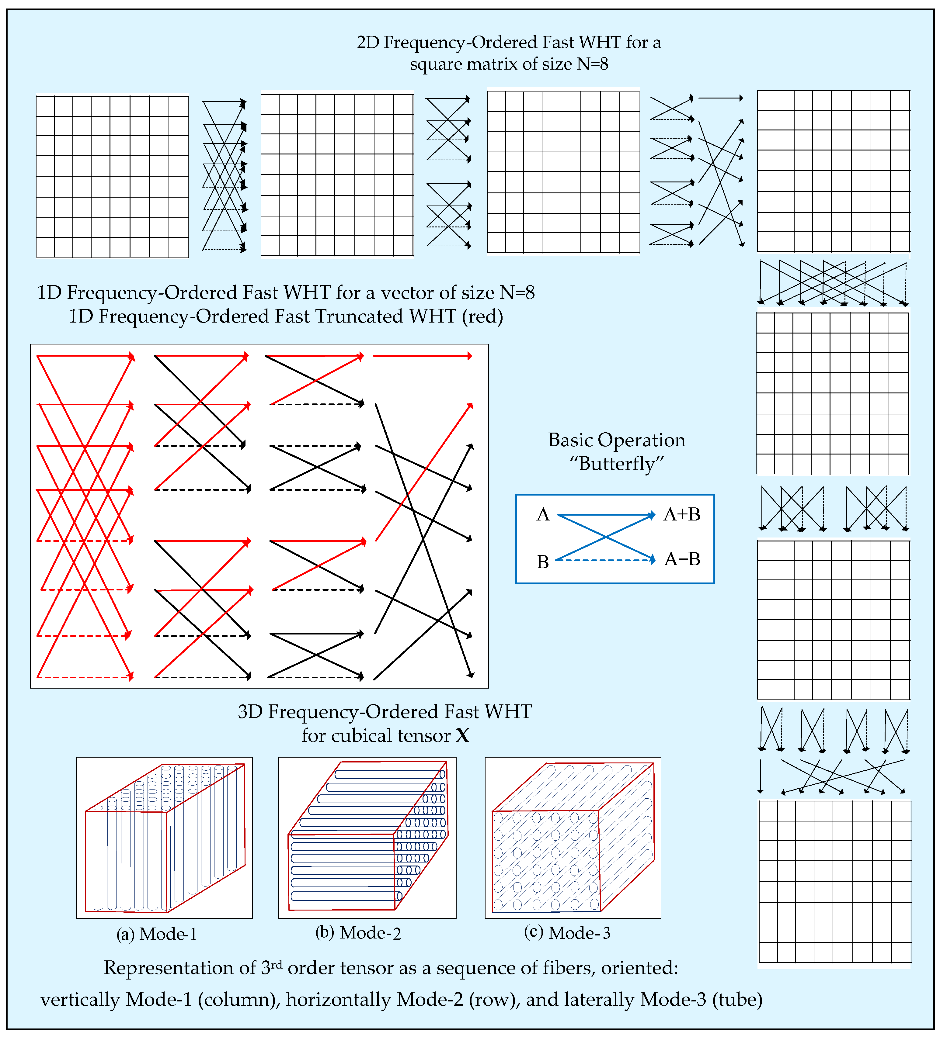
The calculation of 3D FO-FWHT for tensors of the size 8 × 8 × 8 could be executed in accordance with the diagrams, shown in Figure 3. The transform is separable and is executed through consecutive 1D FO-WHT calculations for the columns, rows, and tubes of the tensor X of the size N × N × N, for N = 2ⁿ. To speed up the 1D FO-WHT calculations, the famous “fast” algorithm is used [16]. The number of basic operations “addition” (A_R) needed for the execution of the “fast” 1D FO-WHT (1D FO-FWHT) in correspondence with the computational graph from Figure 3 is ${\mathrm{A}}_{\mathrm{R}}\left(\mathrm{n}\right)=\mathrm{N}\times {\lg }_2\mathrm{N}=2^{\mathrm{n}}\mathrm{n}$. For the case when the “fast“ truncated 1D FO-TWHT (i.e., 1D FO-FTWHT) is used with a reduction (truncation) in some of the output coefficients from N down to 2, the number of “additions” ${\mathrm{A}}_{\mathrm{T}}(\mathrm{n})$ is defined by the relation:

$${\mathrm{A}}_{\mathrm{T}}(\mathrm{n})=\mathrm{N}+\mathrm{N}/2+\mathrm{N}/4+..+\mathrm{N}/2^{\mathrm{n}-1}=\mathrm{N}{\displaystyle \sum _{\mathrm{p}=0}^{\mathrm{n}-1}{2}^{-\mathrm{p}}}=2(2^{\mathrm{n}}-1).$$

(20)

The corresponding graph from Figure 3 is colored in red. In this case, the number of calculations needed for the 1D FO-FWHT compared to 1D FO-FTWHT is defined by the relation below:

$$\mathsf{\psi }(\mathrm{n})=\frac{{\mathrm{A}}_{\mathrm{R}}(\mathrm{n})}{{\mathrm{A}}_{\mathrm{T}}(\mathrm{n})}=\frac{\mathrm{n}}{2(1-2^{-\mathrm{n}})}$$

(21)

Hence, for $\mathrm{n}=3$, $\mathsf{\psi }(3)\approx \hspace{0.17em}1.5$

In accordance with Figure 3, for the 3D WHT transform of the tensor X, it is first divided into N frontal slices (2D matrices). Then, for each column of the sequence of 2D matrices, 1D FWHT is executed, followed by a similar operation for each row of the corresponding transformed matrices. The calculated tensor X comprises all matrices transformed this way. Then, the tensor is divided again, but into N horizontal slices (2D matrices), which are transformed column-by-column through 1D FWHT. After that, on each row of the obtained 2D matrices, 1D TFWHT is applied again (for unfolding mode3 only), which, in correspondence with Equation (20), needs 2(N-1) additions only. Hence, the total number of additions needed to transform the tensor X of the size N × N × N (N = 2ⁿ) through 3D FO-FWHT is correspondingly:

$${\mathrm{A}}_{3\mathrm{D},\mathrm{T}}^{}(\mathrm{n})={\mathrm{N}}^2\hspace{0.17em}[2\mathrm{N}\mathrm{l}{\mathrm{g}}_2\mathrm{N}+2(\mathrm{N}-1)\hspace{0.17em}]=2^{2\mathrm{n}+1}(\mathrm{n}{2}^{\mathrm{n}}+2^{\mathrm{n}}-1)\approx \hspace{0.17em}{2}^{3\mathrm{n}+1}(\mathrm{n}+1).$$

(22)

The total number of additions needed to transform the tensor X of the size N × N × N through 3D WHT is:

$${\mathrm{A}}_{3\mathrm{D}}=3{\mathrm{N}}^3(\mathrm{N}-1)\approx 3\times 2^{4\mathrm{n}}$$

(23)

Hence, the acceleration of the calculations when the modified “fast” 3D FO-WHT (i.e., 3D FO-FWHT) is used, compared to the 3D FO-TFWHT, is:

$${\mathsf{\psi }}_{3\mathrm{D}}(\mathrm{n})=\frac{{\mathrm{A}}_{3\mathrm{D}}^{}(\mathrm{n})}{{\mathrm{A}}_{3\mathrm{D},\mathrm{T}}^{}(\mathrm{n})}\approx \frac{3\times 2^{4\mathrm{n}}}{2\times 2^{3\mathrm{n}}(\mathrm{n}+1)}=1.5\frac{2^{\mathrm{n}}}{\mathrm{n}+1}.$$

(24)

For the case when n = 3, from Equation (24) it follows that ${\mathsf{\psi }}_{3\mathrm{D}}(3)\approx \hspace{0.17em}3$, i.e., the acceleration of the calculations based on the 3D FO-FWHT compared to 3D FO-TFWHT for a tensor X of the size 8 × 8 × 8, is 2.6 times.

5. Comparative Evaluation of 3D-FWHT Computational Complexity

Here, a comparative evaluation of the computational complexity (CC) of the 3D-FWHT is given with respect to the known hierarchical tensor decompositions 3D discrete wavelet transform (3D-DWT) and H-Tucker. For the evaluation, the number of needed basic operations is used. In the general case, the number of additions (A_3H) for the hierarchical 3D-FWHT [14] when N = 2ⁿ (n denotes the number of decomposition levels) is:

$${\mathrm{A}}_{3\mathrm{H}}\left(\mathrm{n}\right)=3\hspace{0.17em}\times 2^{3\mathrm{n}}\mathrm{n}.$$

(25)

The needed number of multiplications for the execution of the direct 3D FWHT is ${\mathrm{l}}_{3\mathrm{H}}(\mathrm{n})=0$. Then, the CC of the 3D FWHT evaluated through the total number of operations ${\mathrm{O}}_{3\mathrm{H}}(\mathrm{n})$ is defined by the relation:

$${\mathrm{O}}_{3\mathrm{H}}(\mathrm{n})={\mathrm{A}}_{3\mathrm{H}}\left(\mathrm{n}\right)+{\mathrm{l}}_{3\mathrm{H}}\left(\mathrm{n}\right)=3\hspace{0.17em}\times 2^{3\mathrm{n}}\mathrm{n}.$$

(26)

The global number of additions and multiplications needed to transform the tensor of a size N × N × N through n-level 3D-DWT with orthogonal filters (3, 5) is correspondingly [14]:

$${\mathrm{A}}_{3\mathrm{W}\mathrm{T}}(\mathrm{n})\hspace{0.17em}=18{\mathrm{N}}^3{\displaystyle {\sum }_{\mathrm{p}=0}^{\mathrm{n}-1}{8}^{-\mathrm{p}}}=20.5\hspace{0.17em}{(2}^{3\mathrm{n}}-1) and {\mathrm{l}}_{3WT}(\mathrm{n})\hspace{0.17em}=24{\mathrm{N}}^3{\displaystyle {\sum }_{\mathrm{p}=0}^{\mathrm{n}-1}{8}^{-\mathrm{p}}}=27.4\hspace{0.17em}(2^{3\mathrm{n}}-1).$$

(27)

Then, the CC of the 3D-DWT is:

$${\mathrm{O}}_{3\mathrm{W}\mathrm{T}}(\mathrm{n})={\mathrm{A}}_{3\mathrm{W}\mathrm{T}}\left(\mathrm{n}\right)+{\mathrm{l}}_{3\mathrm{W}\mathrm{T}}\left(\mathrm{n}\right)\hspace{0.17em}\approx \hspace{0.17em}48\hspace{0.17em}\times 2^{3\mathrm{n}}\mathrm{n}.$$

(28)

The H-Tucker decomposition [2] of the cubical tensor of minimum rank R = 2ⁿ, size N = 2ⁿ, and order d = 3 requires ${\mathrm{O}}_{\mathrm{H}\mathrm{T}}(\mathrm{n})=(3\hspace{0.17em}\times 2^{3\mathrm{n}}+2\times 2^{4\mathrm{n}})$ operations. For the TT decomposition [7], the needed operations for the same tensor are ${\mathrm{O}}_{\mathrm{T}\mathrm{T}}(\mathrm{n})=(3\hspace{0.17em}\times 2^{4\mathrm{n}})$, i.e., the CC is approximately 1.5 times higher than that of the H-Tucker. This is why the H-Tucker transform was selected for the CC comparison with the analyzed 3D deterministic orthogonal transforms.

The relative CC (denoted as $\mathsf{\psi }(\mathrm{n})$) for the execution of the 3D FWHT compared to that of the 3D-DWT and H-Tucker is given below:

$${\mathsf{\psi }}_1(\mathrm{n})={\mathrm{O}}_{3\mathrm{W}\mathrm{T}}(\mathrm{n})/{\mathrm{O}}_{3\mathrm{H}}(\mathrm{n})\hspace{0.17em}=\hspace{0.17em}(48\times 2^{3\mathrm{n}})/(3\times 2^{3\mathrm{n}}\mathrm{n})\approx 16\hspace{0.17em}/\mathrm{n};$$

(29)

$${\mathsf{\psi }}_2(\mathrm{n})={\mathrm{O}}_{\mathrm{H}\mathrm{T}}(\mathrm{n})/{\mathrm{O}}_{3\mathrm{H}}(\mathrm{n})\hspace{0.17em}=2^{3\mathrm{n}}(2^{\mathrm{n}+1}+3)/(3\times 2^{3\mathrm{n}}\mathrm{n})\approx 0.66\times (2^{\mathrm{n}}/\mathrm{n});$$

(30)

The relative CC of the 3D FWHT decreases in inverse proportion to n towards the 3D DWT, while compared to H-Tucker, it grows proportionally to $2^{\mathrm{n}}/\mathrm{n}$. The CC of the 3D FWHT is lower when compared to that of the 3D DWT for levels n < 16, while compared to H-Tucker, it starts to decrease for levels n ≥ 4. In this case, the value of the function ${\mathsf{\psi }}_2(\mathrm{n})\ge 2.6$. The comparison results permit the choosing of the number of hierarchical decomposition levels n, for which the algorithm 3D FWHT is more efficient than 3D DWT and H-Tucker.

6. Global Algorithm for 3D Object Search in a Database of 3D Objects Represented through MLTSP

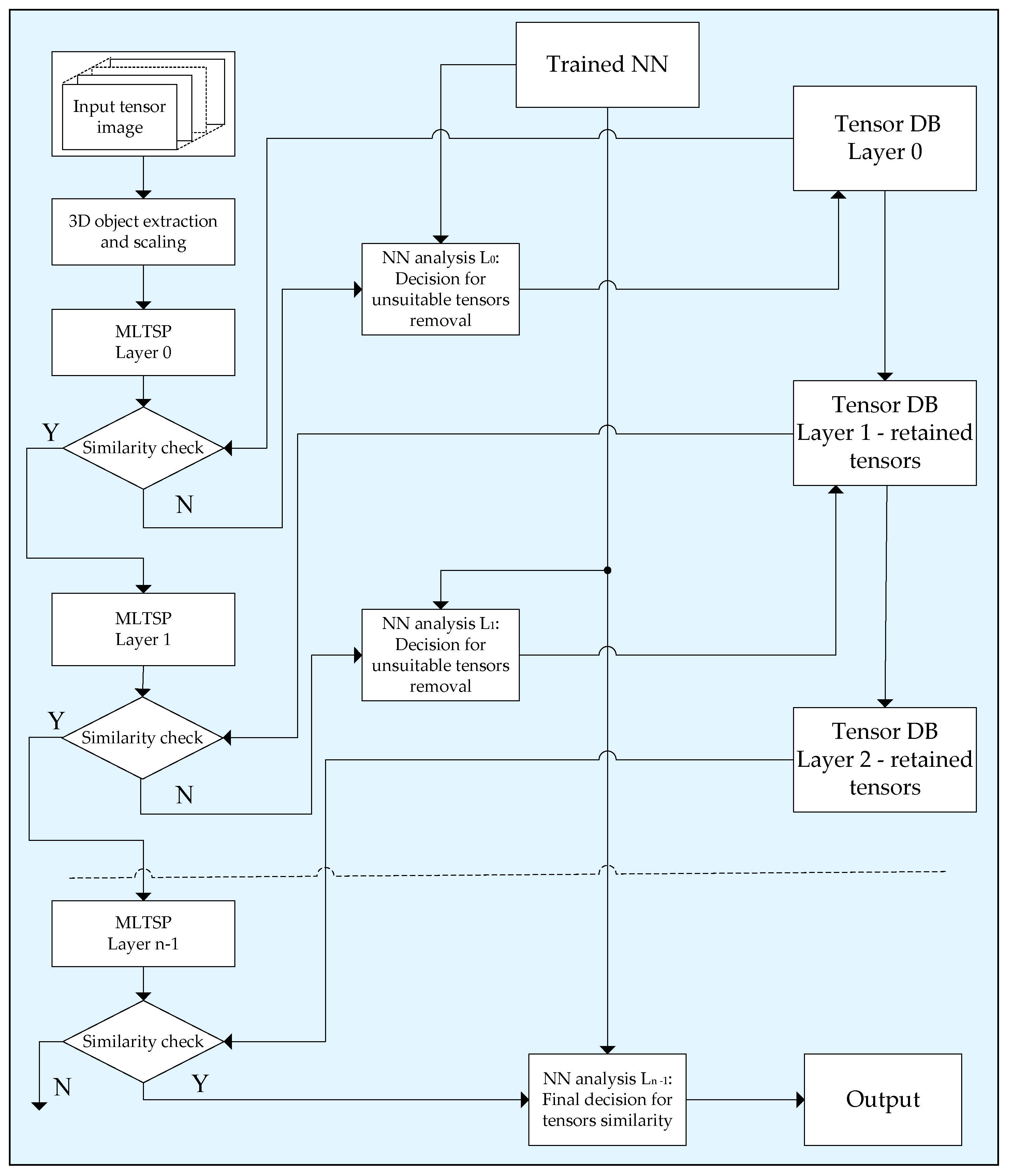
We give here one possible application of the tensor representation based on the n-layer MLTSP, aimed at the accelerated 3D object search in a related database (DB). Such visual information is usually represented by image sequences obtained from various sources: video cameras, multispectral scanners, computer tomography, etc. The authentication degree of the 3D object search is increased significantly compared to the case when 2D image representation only is used. The main problems, which arise when such 3D image systems are created, are related to the high computational complexity of the operations needed for the full search in the DB and the huge number of data needed for the 3D object representation. To overcome these problems, we propose here the global algorithm for accelerated 3D object search, shown in Figure 4.

We suppose that the 3D object DB is already created and contains normalized tensor object representations, each of size N × N × N (for N = 2ⁿ), calculated through the n-layer MLTSP. For the query, the 3D object used is a deep neural network [18]. The segmented object image is scaled so as to match the size of the objects in the DB, and its tensor is represented through the n-layer MLTSP. The basic principle which we used to search for the unknown 3D object is to detect the closest similar objects in the DB through sequential multilayer selection. In the first MLTSP layer (r = 0), the search is full, and, as a result, a group of closest similar objects is selected. The selection is based on the similarity degree between homonymous HTSVD components of the spectrum tensors of the size 2 × 2 × 2 in layers r = 0 of the corresponding MLTSPs. The small size of the compared THSVD components does not demand the use of significant computational resources for similarity evaluations. The search in the next MLTSP layer (r = 1) is also based on the similarity evaluation of the HTSVD components, but for the already selected group in the layer r = 0 only. As a result, the total number of computational operations needed for the similarity evaluation of the query tensor is reduced compared to the group from the previous layer. The search continues in the next MLTSP layers and stops when a 3D object is detected in the DB, whose similarity is higher than a predefined threshold. The thresholds used to select the groups of similar tensors in each layer of MLTSP are defined through training the corresponding neural network (NN).

The similarity degree for a couple of P-dimensional vectors $\mathrm{x}=\hspace{0.17em}{[{\mathrm{x}}_0,{\mathrm{x}}_1,..,\hspace{0.17em}{\mathrm{x}}_{\mathrm{P}-1}]}^{\mathrm{T}}$ and $\mathrm{y}=\hspace{0.17em}{[{\mathrm{y}}_0,{\mathrm{y}}_1,..,\hspace{0.17em}{\mathrm{y}}_{\mathrm{P}-1}]}^{\mathrm{T}}$ is calculated by using the squared cosine similarity (SCSim) criterion [15], defined by the relation:

$$\mathrm{S}\mathrm{C}\mathrm{S}\mathrm{i}\mathrm{m}(\mathrm{x},\mathrm{y})={\left[{\displaystyle \sum _{\mathrm{i}=0}^{\mathrm{P}-1}{\displaystyle \sum _{\mathrm{j}-0}^{\mathrm{P}-1}\mathrm{x}(\mathrm{i})\mathrm{y}(\mathrm{j})}}\right]}^2/\hspace{0.33em}\left[{\displaystyle \sum _{\mathrm{i}-0}^{\mathrm{P}-1}\mathrm{x}{(\mathrm{i})}^2}\right]\times \left[{\displaystyle \sum _{\mathrm{j}=0}^{\mathrm{P}-1}\mathrm{y}{(\mathrm{j})}^2}\right]$$

(31)

To use this criterion for similarity evaluation between a couple of tensors of the same size, first of all, unfolding of the same kind (mode 1, 2, or 3) for each tensor, X and Y, must be executed. In cases that the total number of vectors obtained after the unfolding is Q, for the similarity evaluation, the mean value of SCSim could be used for each couple of vectors x_q and y_q of the same sequential number q = 1, 2, …, Q, which belongs to X and Y, correspondingly:

$$\mathrm{S}\mathrm{C}\mathrm{S}\mathrm{i}\mathrm{m}(\mathbf{X},\mathbf{Y})=\frac{1}{\mathrm{Q}}{\displaystyle \sum _{\mathrm{q}=1}^{\mathrm{Q}}\left\{{\left[{\displaystyle \sum _{\mathrm{i}=0}^{\mathrm{P}-1}{\displaystyle \sum _{\mathrm{j}-0}^{\mathrm{P}-1}{\mathrm{x}}_{\mathrm{q}}(\mathrm{i}){\mathrm{y}}_{\mathrm{q}}(\mathrm{j})}}\right]}^2/\hspace{0.33em}\left[{\displaystyle \sum _{\mathrm{i}-0}^{\mathrm{P}-1}{\mathrm{x}}_{\mathrm{q}}{(\mathrm{i})}^2}\right]\times \left[{\displaystyle \sum _{\mathrm{j}=0}^{\mathrm{P}-1}{\mathrm{y}}_{\mathrm{q}}{(\mathrm{j})}^2}\right]\right\}}$$

(32)

7. Invariant 3D Object Representation, Based on MLTSP with 3D Modified Mellin–Fourier Transform

The description of the 3D object should be invariant to 3D rotations (R) on angles α_r, β_r, γ_r, 3D translation shift (T) in directions x_s, y_s, z_s, 3D scaling (S), and contrast (C) changes. To obtain the invariant representation of a 3D object through MLTSP, the spectrum coefficients at the outputs of the decomposition layers r = 0, 1, …, n−1 must be calculated by using the 3D modified Mellin–Fourier transform (3D MMFT), which is an upgrade from the previous work of the authors, introduced in [15].

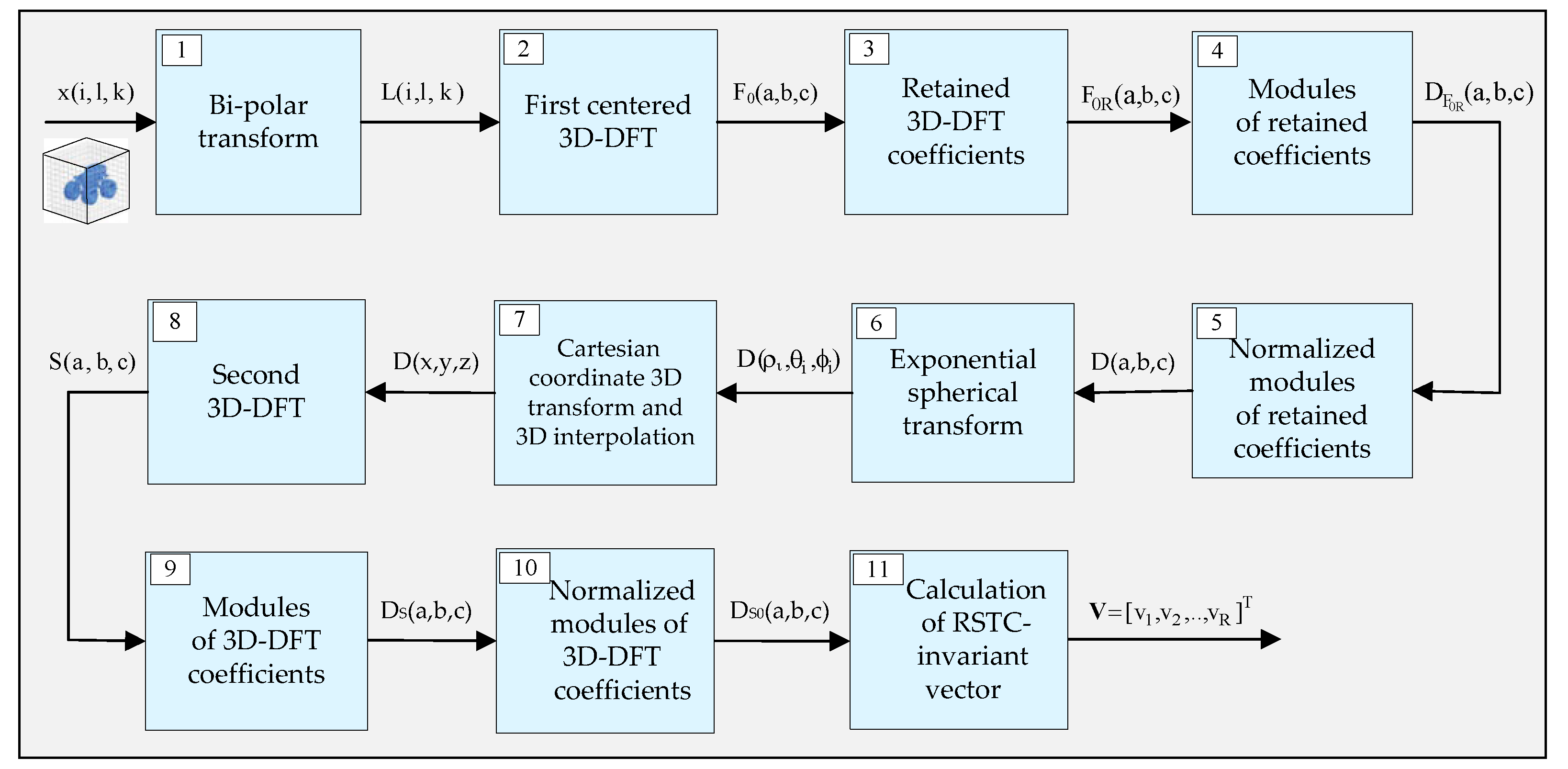
The block diagram of the algorithm for calculation of the direct 3D MMFT spectrum coefficients is shown in Figure 5. The main operations for the 3D MMFT execution are:

(1)

Bi-polar transform of the voxels x(i, l, k) of the input tensor image X:

$$\mathrm{L}(\mathrm{i},\mathrm{l},\mathrm{k})=\mathrm{x}(\mathrm{i},\mathrm{l},\mathrm{k})-(x_{\max }+1)/2 for \mathrm{i}, \mathrm{l}, \mathrm{k}=0,1,.., \mathrm{N}-1,$$

(33)

where x_max is the maximum value in the voxel quantization scale.

(2)

First direct 3D discrete Fourier transform (3D DFT):

$$\mathrm{F}(\mathrm{a},\mathrm{b},\mathrm{c})={\displaystyle \sum _{\mathrm{i}=0}^{\mathrm{N}-1}{\displaystyle \sum _{\mathrm{l}=0}^{\mathrm{N}-1}{\displaystyle \sum _{\mathrm{k}}^{\mathrm{N}-1}\mathrm{L}(\mathrm{i},\mathrm{l},\mathrm{k})\hspace{0.17em}exp\{-\mathrm{j}\hspace{0.17em}(2\pi /\mathrm{N}(ia+\mathrm{l}\mathrm{b}+\mathrm{k}\mathrm{c})]\}}}} for \mathrm{a}, \mathrm{b}, \mathrm{c}=0, 1, .., \mathrm{N}-1$$

(34)

followed by centering of the Fourier coefficients F(a,b,c):

$${\mathrm{F}}_0(\mathrm{a},\mathrm{b},\mathrm{c})=\mathrm{F}(\mathrm{a}-\frac{\mathrm{N}}{2},\mathrm{b}-\frac{\mathrm{N}}{2},\mathrm{c}-\frac{\mathrm{N}}{2}) for \mathrm{a}, \mathrm{b}, \mathrm{c}=0, 1, .., \mathrm{N}-1$$

(35)

(3)

Retaining the centered low-frequency spectrum Fourier coefficients:

$${\mathrm{F}}_{0\mathrm{R}}(\mathrm{a},\mathrm{b},\mathrm{c})=\left\{\begin{array}{c}{\mathrm{F}}_0(\mathrm{a},\mathrm{b},\mathrm{c}),\mathrm{i}\mathrm{f}(\mathrm{a},\mathrm{b},\mathrm{c})\in \mathrm{r}\mathrm{e}\mathrm{t}\mathrm{a}\mathrm{i}\mathrm{n}\mathrm{e}\mathrm{d}\hspace{0.33em}\mathrm{r}\mathrm{e}\mathrm{g}\mathrm{i}\mathrm{o}\mathrm{n};\\ 0\hspace{1em}\hspace{1em}\hspace{1em}-\hspace{1em}\hspace{1em}\mathrm{i}\mathrm{n}\hspace{0.33em}\mathrm{a}\mathrm{l}\mathrm{l}\hspace{0.17em}\mathrm{o}\mathrm{t}\mathrm{h}\mathrm{e}\mathrm{r}\hspace{0.33em}\mathrm{c}\mathrm{a}\mathrm{s}\mathrm{e}\mathrm{s}.\end{array}\right.$$

(36)

The retained coefficients’ region is a cube with a side H ≤ N, which envelopes the center (0,0,0) of the 3D Fourier spectrum (H—even number). For H < N and $\mathrm{a},\mathrm{b},\mathrm{c}=-(\mathrm{H}/2),\hspace{0.17em}-(\mathrm{H}/2)+1,\dots ,-1,\hspace{0.17em}0,\hspace{0.17em}1,\dots ,(\mathrm{H}/2)-1$; this cube contains low-frequency coefficients only.

(4)

Calculation of modules and phases of the retained coefficients ${\mathrm{F}}_{0\mathrm{R}}\hspace{0.17em}(\mathrm{a},\mathrm{b},\mathrm{c})={\mathrm{D}}_{{\mathrm{F}}_{0\mathrm{R}}}(\mathrm{a},\mathrm{b},\mathrm{c}{)\mathrm{e}}^{\mathrm{j}{\mathsf{\phi }}_{{\mathrm{F}}_{0\mathrm{R}}}(\mathrm{a}\hspace{0.17em},\mathrm{b},\mathrm{c})}$:

$$\begin{gathered} {\mathrm{D}}_{{\mathrm{F}}_{0\mathrm{R}}}(\mathrm{a},\mathrm{b},\mathrm{c})=\left|\sqrt{{[{\mathrm{A}}_{{\mathrm{F}}_{0\mathrm{R}}}(\mathrm{a},\mathrm{b},\mathrm{c})]}^2+{[{\mathrm{B}}_{{\mathrm{F}}_{0\mathrm{R}}}(\mathrm{a},\mathrm{b},\mathrm{c})]}^2}\right|, \\ {\mathsf{\phi }}_{{\mathrm{F}}_{0\mathrm{R}}}(\mathrm{a},\mathrm{b},\mathrm{c})=arctan\hspace{0.17em}[{\mathrm{B}}_{{\mathrm{F}}_{0\mathrm{R}}}(\mathrm{a},\mathrm{b},\mathrm{c})/{\mathrm{A}}_{{\mathrm{F}}_{0\mathrm{R}}}(\mathrm{a},\mathrm{b},\mathrm{c})] \end{gathered}$$

(37)

where ${\mathrm{A}}_{0\mathrm{R}}(\mathrm{a},\mathrm{b},\mathrm{c})$ and ${\mathrm{B}}_{0\mathrm{R}}(\mathrm{a},\mathrm{b},\mathrm{c})$ are the real and the imaginary components of ${\mathrm{F}}_{0\mathrm{R}}(\mathrm{a},\mathrm{b},\mathrm{c})$, correspondingly.

(5)

Calculation of the retained coefficients’ normalized modules:

$$\mathrm{D}(\mathrm{a},\mathrm{b},\mathrm{c})=\mathrm{p}\ln {\mathrm{D}}_{{\mathrm{F}}_{0\mathrm{R}}}(\mathrm{a},\mathrm{b},\mathrm{c}) for \mathrm{p}-\mathrm{the} \mathrm{normalization} \mathrm{coefficient};$$

(38)

(6)

Replacement of the orthogonal 3D discretization grid, which contains the voxels $\mathrm{D}(\mathrm{a},\mathrm{b},\mathrm{c})$, by a new grid, defined through 3D logarithmic spherical polar transform (3D LSPT), using the relations below:

$$\mathsf{\rho }=\log \sqrt{{\mathrm{a}}^2+{\mathrm{b}}^2+{\mathrm{c}}^2}, \mathsf{\theta }=\arccos \hspace{0.17em}[\mathrm{c}/\sqrt{{\mathrm{a}}^2+{\mathrm{b}}^2+{\mathrm{c}}^2}], \mathsf{\phi }=\arctan \hspace{0.17em}[\mathrm{b}/\mathrm{a}]$$

(39)

After discretization of $\mathsf{\rho },\mathsf{\theta },\mathsf{\varphi }$, the voxels $\mathrm{D}({\mathsf{\rho }}_{\mathrm{i}},{\mathsf{\theta }}_{\mathrm{j}},{\mathsf{\varphi }}_{\mathrm{j}})$ are obtained where:

$$\begin{gathered} {\mathsf{\rho }}_{\mathrm{i}}=[(\sqrt{2}/2)\mathrm{H}{]}^{\mathrm{i}/\mathrm{H}} for \mathrm{i}=1, 2, .., \mathrm{H}; \\ {\mathsf{\theta }}_{\mathrm{j}}\hspace{0.17em}=(2\pi /\mathrm{H})\mathrm{j} and {\mathsf{\varphi }}_{\mathrm{j}}=(2\pi /\mathrm{H})\mathrm{j} for \mathrm{j}=(-\mathrm{H}/2),.,-1,0,1,.,(\mathrm{H}/2)-1. \end{gathered}$$

(40)

Here, instead of the 3D LSPT given in Equation (32), we used the 3D exponential polar transform (3D EPT) from Equation (33), which gives a higher density of the retained voxels $\mathrm{D}(\mathrm{a},\mathrm{b},\mathrm{c})$ around the origin (0,0,0) of the discretization grid $({\mathsf{\rho }}_{\mathrm{i}},{\mathsf{\theta }}_{\mathrm{j}},{\mathsf{\varphi }}_{\mathrm{j}})$.

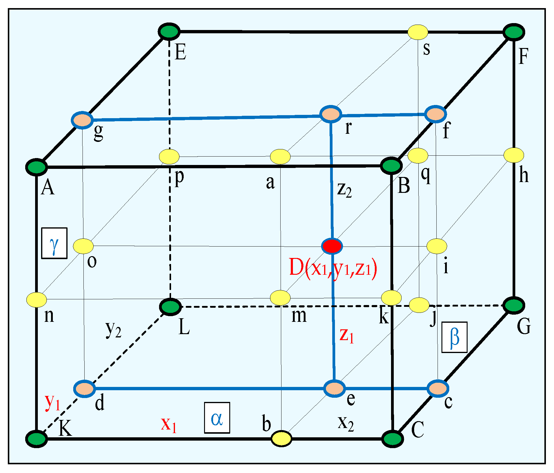
(7)

Replacement of the discretization grid for voxels $\mathrm{D}({\mathsf{\rho }}_{\mathrm{i}},{\mathsf{\theta }}_{\mathrm{j}},{\mathsf{\varphi }}_{\mathrm{j}})$ defined through 3D EPT, by the orthogonal discretization 3D grid for voxels D(x,y,z), calculated through trilinear interpolation (Figure 6). In this case, each interpolated voxel D(x₁,y₁,z₁) is calculated taking into consideration the closest eight neighbor voxels on the grid:

$$\mathrm{D}({\mathrm{x}}_1,{\mathrm{y}}_1,{\mathrm{z}}_1)=(1/{\mathrm{H}}^3)\{{\mathrm{z}}_1[{\mathrm{x}}_1({\mathrm{y}}_1\mathrm{B}+{\mathrm{y}}_2\mathrm{F})+{\mathrm{x}}_2({\mathrm{y}}_1\mathrm{E}+{\mathrm{y}}_2\mathrm{A})]+{\mathrm{z}}_2[{\mathrm{y}}_1({\mathrm{x}}_1\mathrm{G}+{\mathrm{x}}_2\mathrm{L})+{\mathrm{y}}_2({\mathrm{x}}_1\mathrm{C}+{\mathrm{x}}_2\mathrm{K})]\}$$

(41)

where A, B, C, K, E, F, G, L—neighboring voxels from the discretization grid $(\mathrm{x},\mathrm{y},\mathrm{z})$;

α, β, γ—distances between the eight neighboring voxels in directions x, y, z;

D(x₁,y₁,z₁)—linearly interpolated voxel for ${\mathrm{x}}_1=\mathsf{\alpha }-{\mathrm{x}}_2$, ${\mathrm{y}}_1=\mathsf{\beta }-{\mathrm{y}}_2$, ${\mathrm{z}}_1=\mathsf{\gamma }-{\mathrm{z}}_1$;

The obtained results are the voxels D(x,y,z) of the interpolated output tensor D for x, y, z = 0, 1, 2, .., H − 1.

(8)

Second direct 3D DFT for a tensor D, with voxels D(x,y,z):

$$\mathrm{S}(\mathrm{a},\mathrm{b},\mathrm{c})=(1/{\mathrm{H}}^3){\displaystyle \sum _{\mathrm{x}=0}^{\mathrm{H}-1}{\displaystyle \sum _{\mathrm{y}=0}^{\mathrm{H}-1}{\displaystyle \sum _{\mathrm{z}=0}^{\mathrm{H}-1}\mathrm{D}(\mathrm{x},\mathrm{y},\mathrm{z})\hspace{0.17em}exp\{-\mathrm{j}\hspace{0.17em}(2\pi /\mathrm{N}(xa+\mathrm{y}\mathrm{b}+\mathrm{z}\mathrm{c})]\}}}} for \mathrm{a},\mathrm{b},\mathrm{c}=0,1,..,\mathrm{H}-1.$$

(42)

(9)

Calculation of the complex coefficient $\mathrm{S}(\mathrm{a},\mathrm{b},\mathrm{c})$ modules:

$${\mathrm{D}}_{\mathrm{S}}(\mathrm{a},\mathrm{b},\mathrm{c})=\left|\sqrt{{[{\mathrm{A}}_{\mathrm{S}}(\mathrm{a},\mathrm{b},\mathrm{c})]}^2+{[{\mathrm{B}}_{\mathrm{S}}(\mathrm{a},\mathrm{b},\mathrm{c})]}^2+{[{\mathrm{C}}_{\mathrm{S}}(\mathrm{a},\mathrm{b},\mathrm{c})]}^2}\right|,$$

(43)

where ${\mathrm{A}}_{\mathrm{S}}(\mathrm{a},\mathrm{b},\mathrm{c})$, ${\mathrm{B}}_{\mathrm{S}}(\mathrm{a},\mathrm{b},\mathrm{c})$, and ${\mathrm{C}}_{\mathrm{S}}(\mathrm{a},\mathrm{b},\mathrm{c})$ are the real and the imaginary components of $\mathrm{S}(\mathrm{a},\mathrm{b},\mathrm{c})$, correspondingly.

(10)

Calculation of the normalized modules ${\mathrm{D}}_{{\mathrm{S}}_0}(\mathrm{a},\mathrm{b},\mathrm{c})$ of the Fourier coefficients $\mathrm{S}(\mathrm{a},\mathrm{b},\mathrm{c})$:

$${\mathrm{D}}_{{\mathrm{S}}_0}(\mathrm{a},\mathrm{b},\mathrm{c})={\mathrm{x}}_{max}\times \hspace{0.17em}[({\mathrm{D}}_{\mathrm{S}}(\mathrm{a},\mathrm{b},\mathrm{c})/{\mathrm{D}}_{\mathrm{S}max}(\mathrm{a},\mathrm{b},\mathrm{c}))],$$

(44)

where ${\mathrm{D}}_{\mathrm{S}max}(\mathrm{a},\mathrm{b},\mathrm{c})$ is the module of the coefficient $\mathrm{S}(\mathrm{a},\mathrm{b},\mathrm{c})$ with a maximum value for $\mathrm{a},\mathrm{b},\mathrm{c}=0,1,..,\mathrm{H}-1$.

(11)

Calculation of the vector for RSTC-invariant 3D object representation based on the coefficients ${\mathrm{D}}_{{\mathrm{S}}_0}(\mathrm{a},\mathrm{b},\mathrm{c})$ of highest energy in the amplitude spectrum 3D MMFT, for $\mathrm{a},\mathrm{b},\mathrm{c}=0,1,..,\mathrm{H}-1$. The v_m components for m = 1, 2, .., R of the corresponding RSTC-invariant vector $V=\hspace{0.17em}{[{\mathrm{v}}_1,{\mathrm{v}}_2,..,\hspace{0.17em}{\mathrm{v}}_{\mathrm{R}}]}^{\mathrm{T}}$ are defined by coefficients ${\mathrm{D}}_{{\mathrm{S}}_{0\mathrm{R}}}(\mathrm{a},\mathrm{b},\mathrm{c})$, arranged as a 1D massif after scanning the 3D-MMFT spectrum in the frame of the 3D mask area with R < H³ voxels ${\mathrm{D}}_{{\mathrm{S}}_0}(\mathrm{a},\mathrm{b},\mathrm{c})$.

The main advantages of 3D MMFT compared to other famous spectrum 3D object descriptors [19,20,21,22] are that it is an RSTC invariant, and the features’ space dimensionality is reduced. This is why the approach based on MLTSP with embedded 3D MMFT accelerates the search of 3D objects in tensor DBs and ensures higher identification accuracy.

8. Conclusions

In this work, a new approach is proposed for 3D tensor representation through MLTSP with embedded 3D FO-FWHT and HTSVD, or 3D FO-FWHT and 3D-MMFT depending on the application, for example, information redundancy reduction in the input tensor, or an accelerated 3D object search in a tensor DB. In both cases, the main advantages of the MLTSP algorithms are the low computational complexity, the high flexibility regarding the choice of their parameters, and the ability for information redundancy reduction in the input tensor. These qualities have good potential for application in various areas where multidimensional signals and images are concerned.

Our future work will be focused on MLTSP modeling with various kinds of 3D OT and on the investigation of spectrum pyramid applications in different areas of tensor image processing, analysis, and computer vision. The future investigation of the MLTSP application in deep learning architectures is extremely promising.