
Interval Estimation for the Two-Parameter Exponential Distribution Based on the Upper Record Values


Department of Statistics, Tamkang University, Tamsui, Taipei 251301, Taiwan
Symmetry 2022, 14(9), 1906; https://doi.org/10.3390/sym14091906
Submission received: 22 August 2022
/
Revised: 3 September 2022
/
Accepted: 8 September 2022
/
Published: 12 September 2022
(This article belongs to the Special Issue Skewed (Asymmetrical) Probability Distributions and Applications across Disciplines II)
Abstract
:Using the data for upper record values, the interval estimation for the scale parameter of two-parameter exponential distribution is presented. In addition, two methods for the joint confidence region of two parameters are proposed. In terms of confidence region area, the simulation comparison of two methods of the confidence region is performed in this paper. The criterion of minimum confidence region area is used to obtain the optimal method of the confidence region. To illustrate our proposed interval estimation methods, one biometrical example is used and the corresponding confidence interval length and confidence region area are also calculated. Our research topic is related to the asymmetrical probability distributions and applications across disciplines.
1. Introduction
In lifetime test experiments and reliability analysis, the exponential distribution is widely used in modelling the lifetime data. Wu [1] proposed a modified one-stage multiple comparison procedure for comparing exponential location parameters with the control when the scale parameters are unequal (under heteroscedasticity). Please see Johnson and Kotz [2], Bain [3], Lawless and Singhal [4] and Zelen [5] for other applications of exponential distributions. Other than exponential distributions, Shafiq et al. [6] identified an effective statistical distribution called the modified Kies Frechet (MKIF) model for examining COVID-19 mortality rates in Canada and the Netherlands. El-Khatib and Hatemi-J [7] suggested formulas to make the valuation of options and the underlying hedging strategies during financial crisis more precise. Alzaatreh et al. [8] presented a new distribution called Weibull–Pareto distribution and the properties of this distribution are obtained and illustrated by some real data sets.
Now we start to define the upper record value data as follows: let be a random sample from a two-parameter exponential distribution. We treated as an upper record value if for all . The observed time point for the first upper record value is denoted as . Then the observed time point for the nth upper record value is denoted as , where . Then is called the sequence of upper record values of the original sequence . An analogous definition of lower record values is obtained by changing the sign of ‘>’ to the sign of ‘<’. In this study, we were only concerned with the case of upper record values. However, all results should be applicable to the case of lower record values. Record values data appeared in many real life applications, such as life-tests, weather, sports, economics, and so on. In the last two decades, many authors had studied the statistical inference based on the record values. (See for example, Al-Hussaini and Ahmad [9].) For simplicity, we denote the sequence of upper record values as .
Since some statistical properties of exponential distribution depend on their two parameters, the development of the confidence region for two parameters is necessary. Asgharzadeh et al. [10] proposed interval estimation for the Pareto distribution using record values. For the inverse Weibull distribution, Jana and Bera [11] proposed the interval estimation of multicomponent stress–strength reliability. Wu [12] proposed the Bayesian interval estimation for the two-parameter exponential distribution based on the right type II censored sample. Wu [13] proposed the Bayesian interval estimation for the two-parameter exponential distribution using the progressive type II censored sample. In this research, we would like to propose the confidence interval of the scale parameter for two-parameter exponential distribution using the upper record value data. Two methods of joint confidence region for two parameters are also proposed. The Monte Carlo simulation method is used to assess the performance of all interval estimation results in terms of the length of the confidence interval or the area of the confidence region. At last, we give a biometrical example to illustrate the proposed methods.
2. Interval Estimation and Confidence Region for Two Parameters
At first, we consider a random variable X following a two-parameter exponential distribution with scale parameter and location parameter . Its probability density function (pdf) is given by:
Its cumulative distribution function (cdf) is given by .
Consider the sequence of upper record values following the two-parameter exponential distribution. From Arnold et al. [14], the joint pdf of is:
The log-likelihood function can be obtained as:
Since the log-likelihood function is an increasing function of µ, the maximum likelihood estimator (MLE) for µ is given by . Substituting the MLE of µ into the log-likelihood function and taking the derivative of the log-likelihood function with respect to , then we have .
Equating the above equation to zero, then the MLE of can be obtained as:
After the transformations of we can obtain a sequence of upper record values from a standard exponential distribution. Due to the property of being memoryless for exponential distribution, it is apparent that the differences between two successive upper record values will be independently and identically distributed (iid) from standard exponential distribution. That is, are independent identically distributed from standard exponential distribution.
In order to build the interval estimation for parameters, two sets of pivotal quantities are considered. The first set of pivotal quantities consists of and . The distributions for these two pivotal quantities are independently chi-squared distributed with and degrees of freedom, respectively. We denote the chi-squared distribution with degrees of freedom v as and the F distribution with degrees of freedom v1 and v2 as F(v1,v2). Furthermore, the second set of pivotal quantities consists of and . The distributions of these two pivotal quantities are and . The distributions of all pivotal quantities are not a function of parameters. Utilizing the pivotal quantity , we can build the confidence interval for the scale parameter θ as follows:
Proposition 1.
Considering a sequence of upper record values denoted by following the two-parameter exponential distribution with parameters and , the () 100% confidence intervals of the scale parameter θ is:
where is the right-tailed percentile for chi-squared distribution with degrees of freedom.
Proof of Proposition 1.
Since the distribution of the pivotal quantity is , we have:
Utilizing the first set of pivotal quantities and , we can construct the confidence region of two parameters in Theorem 1 and it is called Method 1. □
Theorem 1.
Considering a sequence of upper record values denoted by following the two-parameter exponential distribution with parameters and , the ()100% joint confidence region of two parameters and is given by:
where and and represent the right-tailed and percentile for the chi-squared distribution with degrees of freedom.
Proof of Theorem 1.
Since the distributions of the first set of pivotal quantities are independent and and , we have
The area for the confidence region based on Method 1 denoted by Area1 is obtained as follows:
where and .
Utilizing the second set of pivotal quantities and , we can construct the confidence region of two parameters in Theorem 2 and it is called Method 2. □
Theorem 2.
Considering a sequence of upper record values following the two-parameter exponential distribution with parameters and , the () 100% joint confidence region of two parameters and is given by:
where and and represent the right-tailed and percentile for F distribution with 2 and 2n-2 degrees of freedom; and represent the right-tailed and percentile for the chi-squared distribution with degrees of freedom.
Proof of Theorem 2.
Since the distributions of the second set of pivotal quantities are independent and and , we have:
The area for the confidence region based on Method 2 denoted by Area2 is obtained as follows:
where and . □
3. Simulation Study
Using Proposition 1 and Theorems 1–2 (Methods 1–2), the simulated average confidence length and confidence area with the nominal confidence coefficient 1-α = 0.90, 0.95 for n = 1(1)10(10)30, 60 are obtained in Table 1 based on 5000 simulation runs. From Table 1, we found that the confidence length and confidence area are decreasing when sample size n is increasing for fixed 1-α = 0.90, 0.95 and increasing when confidence level 1-α is increasing for fixed n. As for the confidence region, Method 2 has better performance than Method 1 when 2 for 1-α = 0.90 and when 3 for 1-α = 0.95 in terms of shorter confidence area. Therefore, Method 2 is recommended for use for the confidence region of two parameters when 2 for 1-α = 0.90 and when 3 for 1-α = 0.95 and Method 1 is recommended for use only when n = 1 for 1-α = 0.90 when n = 1,2 for 1-α = 0.95. We also found that the simulation results indicate that all proposed methods can reach the nominal confidence coefficient.
4. A Biometrical Example
In Proschan [15], the data for times between successive failures of air conditioning equipment in a Boeing 70 airplane are used to illustrate the proposed methods in Proposition 1 and Theorems 1–2. The data are 57,48,74,29,12,70,21,29, 326,59,27,153,26, 386,502. It is assumed that the data fit an exponential distribution. The sequence of upper record values are = {57,74,326,386,502}.
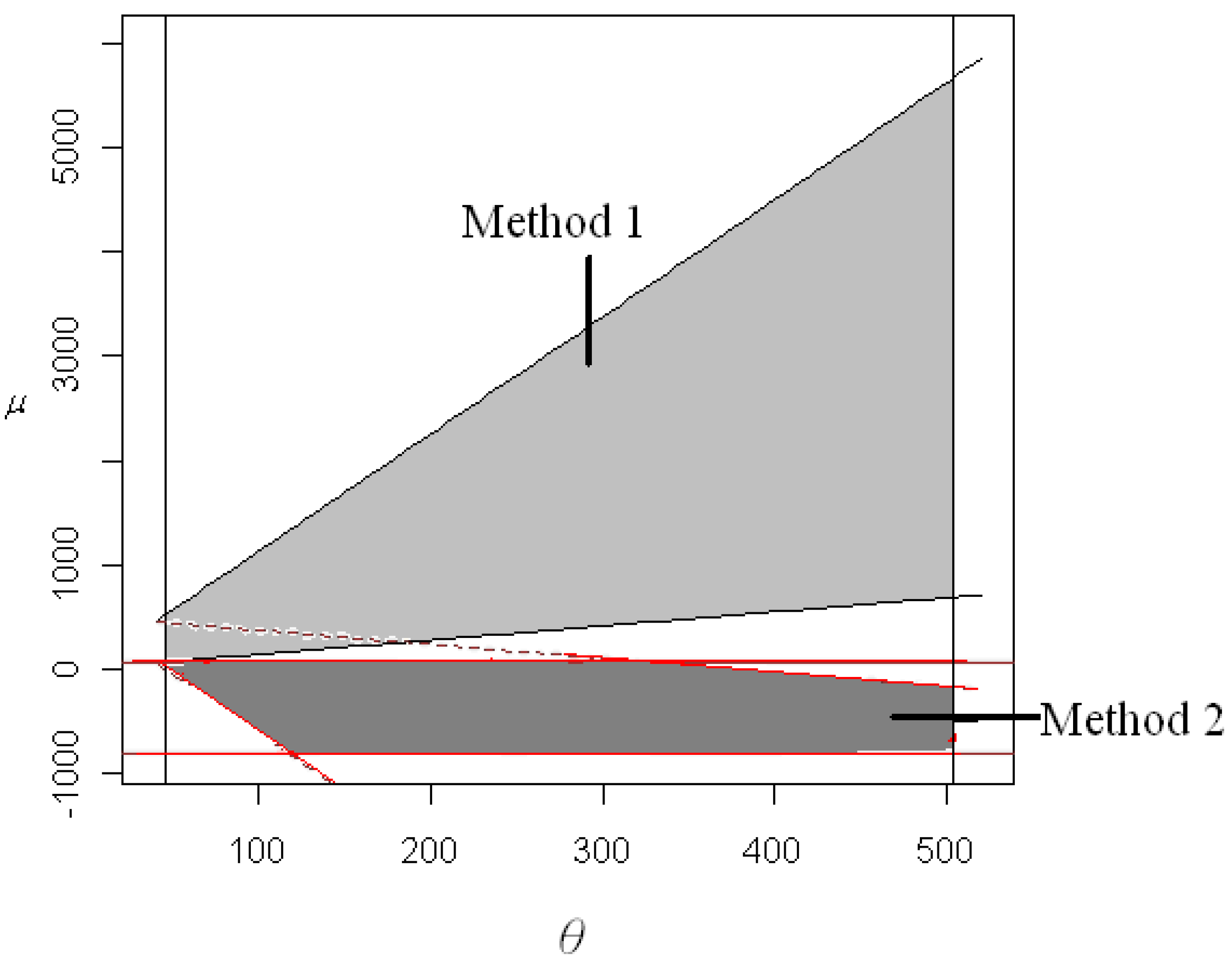
By Proposition 1, the 95% confidence interval for θ is obtained as (50.75695, 408.30731) with confidence length 357.5504. By Theorem 1 (Method 1), the 95% joint confidence region for θ and is given by:
with area 548,019.8.
By Theorem 2 (Method 2), the 95% confidence region is given by with area 505,305.9. The confidence regions for two parameters obtained by Method 1 and Method 2 are plotted in Figure 1.
From Figure 1, the users can see that the area obtained by Method 2 is smaller than the one obtained by Method 1. Therefore, Method 2 is recommended for the construction of the confidence region of two parameters rather than Method 1 for this example.
5. Conclusions
This paper proposed the confidence interval for the scale parameter θ and two methods for the development of the confidence region of θ and for the two-parameter exponential distribution based on the upper record value data. From the simulation comparison study, we recommend Method 2 rather than Method 1 for the construction of the confidence region for two parameters under most cases. We also found that all proposed methods can reach the nominal confidence coefficient. At last, we employed one biometrical example to illustrate the application of the proposed interval estimation for two parameters in this paper.
Funding
This research and the APC are funded by [National Science and Technology Council, Taiwan] NSTC 111-2118-M-032-003-MY2.
Data Availability Statement
The data presented in this study are openly available in Proschan [15].
Conflicts of Interest
The author declares no conflict of interest.
References
- Wu, S.F. A modified one stage multiple comparison procedure of exponential location parameters with the control under heteroscedasticity. Commun. Stat.-Theory Methods 2021. [Google Scholar] [CrossRef]
- Johnson, N.L.; Kotz, S. Continuous Univariate Distributions; John Wiley & Sons, Inc.: New York, NY, USA, 1970. [Google Scholar]
- Bain, L.J. Statistical Analysis of Reliability and Life Testing Models; Marcer Dekker: New York, NY, USA, 1978. [Google Scholar]
- Lawless, J.F. Statistical Models and Methods for Lifetime Data; John Wiley & Sons, Inc.: New York, NY, USA, 1982. [Google Scholar]
- Zelen, M. Application of exponential models to problems in cancer research. J. R. Stat. Soc. 1966, 129, 368–398. [Google Scholar] [CrossRef]
- Shafiq, A.; Lone, S.A.; Sindhu, T.N.; Khatib, Y.E.; Al-Mdallal, Q.M.; Muhammad, T. A new modified Kies Fréchet distribution: Applications of mortality rate of COVID-19. Results Physics 2021, 28, 104638. [Google Scholar] [CrossRef] [PubMed]
- El-Khatib, Y.; Hatemi-J, A. Option valuation and hedging in markets with a crunch. J. Econ. Stud. 2017, 44, 801–815. [Google Scholar] [CrossRef]
- Alzaatreh, A.; Famoye, F.; Lee, C. Weibull-Pareto Distribution and Its Applications. Commun. Stat.-Theory Methods 2013, 42, 1673–1691. [Google Scholar] [CrossRef]
- Al-Hussaini, E.K.; Ahmad, A.A. On Bayesian Interval Prediction of Future Records. Test 2003, 12, 79–99. [Google Scholar] [CrossRef]
- Asgharzadeh, A.; Abdi, M.; Kuş, C. Interval estimation for the two-parameter Pareto distribution based on record. Selçuk J. Appl. Math. 2011, 149–161. [Google Scholar]
- Jana, N.; Bera, S. Interval estimation of multicomponent stress–strength reliability based on inverse Weibull distribution. Math. Comput. Simul. 2022, 191, 95–119. [Google Scholar] [CrossRef]
- Wu, S.F. Bayesian interval estimation for the two-parameter exponential distribution based on the right type II censored sample. Symmetry 2022, 14, 352. [Google Scholar] [CrossRef]
- Wu, S.F. Interval estimation for the two-parameter exponential distribution under progressive type II censoring on the Bayesian approach. Symmetry 2022, 14, 808. [Google Scholar] [CrossRef]
- Arnold, B.C.; Balakrishnan, N.; Nagaraja, H.N. Records; John Wiley & Sons, Inc.: New York, NY, USA, 1998. [Google Scholar]
- Proschan, F. Theoretical explanation of observed decreasing failure rate. Technometrics 1963, 3, 375–383. [Google Scholar] [CrossRef]
Figure 1.
As shown, 95% confidence region for the example under Method 1 and Method 2.


Table 1.
The average length and area for the interval estimation of the exponential distribution with (, ) = (0,1) under 1-α = 0.90 and 0.95.
Table 1.
The average length and area for the interval estimation of the exponential distribution with (, ) = (0,1) under 1-α = 0.90 and 0.95.
| 1-α = 0.90 | 1-α = 0.95 | |||||
|---|---|---|---|---|---|---|
| n | Length | Method 1 | Method 2 | Length | Method 1 | Method 2 |
| 1 | 18.9442 | 5170.463 | 5672.394 | 40.1069 | 28621.48 | 38499.85 |
| 2 | 5.2178 | 181.8382 | 167.7742 | 7.8828 | 471.5438 | 474.2633 |
| 3 | 3.2142 | 55.4781 | 50.0454 | 4.4151 | 113.3213 | 106.0673 |
| 4 | 2.4160 | 29.6365 | 26.8569 | 3.1991 | 54.3921 | 50.1530 |
| 5 | 1.9952 | 19.8614 | 18.1598 | 2.6003 | 35.3613 | 32.5916 |
| 6 | 1.7454 | 15.3585 | 14.1663 | 2.2028 | 24.9928 | 23.1242 |
| 7 | 1.5387 | 12.0971 | 11.2444 | 1.9497 | 19.7239 | 18.3398 |
| 8 | 1.4171 | 10.4444 | 9.7725 | 1.7536 | 16.2681 | 15.2019 |
| 9 | 1.2945 | 8.9408 | 8.4128 | 1.5989 | 13.7533 | 12.9117 |
| 10 | 1.2020 | 7.8545 | 7.4262 | 1.4980 | 12.3047 | 11.6006 |
| 15 | 0.9339 | 5.3172 | 5.109 | 1.1449 | 7.9318 | 7.5936 |
| 20 | 0.7942 | 4.2413 | 4.1122 | 0.9625 | 6.153 | 5.9454 |
| 30 | 0.6299 | 3.1236 | 3.0579 | 0.7617 | 4.4811 | 4.3750 |
| 60 | 0.4365 | 2.0251 | 2.0031 | 0.5219 | 2.8227 | 2.7876 |
Publisher’s Note: MDPI stays neutral with regard to jurisdictional claims in published maps and institutional affiliations. |
© 2022 by the author. Licensee MDPI, Basel, Switzerland. This article is an open access article distributed under the terms and conditions of the Creative Commons Attribution (CC BY) license (https://creativecommons.org/licenses/by/4.0/).
Share and Cite
MDPI and ACS Style
Wu, S.-F. Interval Estimation for the Two-Parameter Exponential Distribution Based on the Upper Record Values. Symmetry 2022, 14, 1906. https://doi.org/10.3390/sym14091906
AMA Style
Wu S-F. Interval Estimation for the Two-Parameter Exponential Distribution Based on the Upper Record Values. Symmetry. 2022; 14(9):1906. https://doi.org/10.3390/sym14091906
Chicago/Turabian StyleWu, Shu-Fei. 2022. "Interval Estimation for the Two-Parameter Exponential Distribution Based on the Upper Record Values" Symmetry 14, no. 9: 1906. https://doi.org/10.3390/sym14091906
Note that from the first issue of 2016, this journal uses article numbers instead of page numbers. See further details here.