ConvLSTM Coupled Economics Indicators Quantitative Trading Decision Model

Abstract

Time series prediction methods based on deep learning have been widely used in quantitative trading. However, the price of virtual currency represented by Bitcoin has random fluctuation characteristics, which is extremely misleading for time series prediction. In this paper, a virtual currency quantitative trading model is established, which uses a convolution long short term memory (ConvLSTM) deep learning method to predict the transaction price, and uses the evaluation model composed of Chandler momentum oscillator (CMO), percentage price oscillator (PPO), stop and reverse(SAR) and other economic indicators to make further decisions. The model quantitatively classifies the random wandering characteristics by fusing economic indicators and extracts the symmetric economic laws among them, making full use of deep learning methods to extract spatial and temporal features within the data. The 2016–2021 Bitcoin value dataset published on Kaggle was used for simulated investment. The results show that compared with other existing decision models, it shows better performance and robustness, and shows good stability in dealing with the interdependence of long-term and short-term data. Our work provides a new idea for short-term prediction of long time series data affected by multiple complex factors: coupling deep learning methods with prior knowledge to complete prediction and decision making.

1. Introduction

In recent years quantitative trading has become a hot topic with the development of virtual currencies. Quantitative trading allows the use of computer technology for the analysis of quantitative data to obtain more objective trading results and capture market opportunities. Initially, people used random regression models, decision tree models and MLP networks to implement quantitative trading. As society progresses and the economy develops, the factors affecting quantitative trading tasks, such as virtual currencies, have become increasingly complex. The price fluctuations of virtual currencies are a type of randomly wandering data in continuous time, with prices at each time point being random, and only by identifying the hidden patterns connecting these price fluctuations is it possible to make short-term predictions of prices. The continuous development of deep learning offers the possibility to solve this problem.

In this paper, we propose a quantitative trading model with decision-making capability, first using ConvLSTM for processing bitcoin price volatility predictions, and then using economic indicators to make decisions on the buy and sell operations of the model. The CNN network extracts features from the input price data and uses the output of the CNN layer as the input part of the LSTM layer for feature learning of time series. One of the LSTM layers has six hidden layer dimensions and uses a structure of two LSTM tandems. Eighty per cent of the dataset was used as the training set and twenty per cent as the test set, and the model was trained using Adam as the optimizer and MSE loss function for 1000 epochs of model convergence. The results show that incorporating economic indicators as a circular exit mechanism for the ConvLSTM model can significantly reduce the risk of investment, and the economic indicators also help to enhance the robustness of the ConvLSTM prediction.

2. Related Work

2.1. Stochastic Regression Model

In the early days, linear regression and simple non-linear models were used to predict financial returns as there was a single factor affecting financial transactions. Since its proposed introduction, ARIMA has rapidly become the most popular time series forecasting model due to its efficient performance.

Brian K. Nelson [1] used the ARIMA model for time series analysis with satisfactory results. Autoregressive models are also an effective method used in time series analysis to describe and model time series data. Short-time relationships are essential for autoregressive models, but the global modelling of the model is not obvious, and Torsten Ullrich [2] analyses the global structure of autoregressive models through the derivation of a closed form. Furthermore, the latest techniques are extended using eigenanalysis and ordinary differential equations to reveal important global properties of autoregressive models that are reflected in time series data and provide decision support in the selection of models describing time series.

Roberto Baragona and colleagues [3]. Propose a comprehensive seasonal integral periodic autoregressive model that not only provides the user with a detailed model for data description and forecasting purposes but also suggests the presence of seasonal unit roots, the validity of which has been highlighted by extensive simulation experiments.

In 2021 Nikita Andriyanov et al. [4]. Presented an analysis of the impact of restrictive measures on disease transmission, predicting the growth of disease based on a double stochastic model, a multi-root characteristic equation model and an autoregressive model with a stochastic process. The analysis showed that the responses adopted, although more restrictive, were effective in reducing the rate of disease transmission. This work shows that autoregressive models are effective for both the stochastic and time-series nature of disease migration and transmission data.

Over a long period, it has been shown that linear regression models have good performance in time series forecasting but are not effective when used for quantitative trading, and the non-linear nature of highly volatile cryptocurrency prices shows significant errors for short-term forecasting of long-term time series. G. Peter Zhang [5] proposed a hybrid approach combining ARIMA and ANN models for linear and non-linear models. Dunis et al. [6] used ARMA models as a linear benchmark to compare with non-linear models, such as multilayer perceptron (MLP) and higher order neural networks (HONN) and tested them on precious metals market data from January 2001 to May 2006 in a trading simulation. Trading simulation tests on precious metals market data from May 2001 to May 2006 and concluded that the non-linear model significantly outperformed the linear model in financial simulation trading.

2.2. Deep Learning Model

Quantitative trading using deep learning has been one of the hot issues in the field of deep learning applications at present. To deal with the extraction of temporal and contextual information in the data (Pascanu et al. [7]) proposed RNN, the parameters of the hidden layer in RNN not only depends on the current input but also on the value of the hidden layer at the previous moment, such a method can handle the sequence information well. However, due to the activation function used in deep learning, if the gradient between hidden layers is small in the backpropagation process, the smaller the accumulated value when calculating the gradient concatenation calculation, the smaller the product value is when the length of the sequence is longer, even close to 0 [8]. Therefore, RNN is difficult to learn information at a long distance when dealing with long-time series data prediction and has short-term memory capability. To solve this problem, Hochreiter et al. [9] proposed long short-term memory (LSTM), which incorporates a memory cell and gating unit in this network, where the gating unit consists of input gate, output gate and forgetting gate, through which gating determines which information needs to be forgotten, added and carried forward. Pichl (2017) et al. [10] Showed that recurrent neural networks (RNNs) and long short-term memory (LSTM) can produce higher prediction accuracy relative to machine learning for predicting bitcoin price fluctuations. McNally (2018) et al. [11] Showed that RNN and LSTM neural networks predict prices better than traditional multilayer perceptrons (MLPs). The gated unit structure allows LSTM networks to learn the hidden long- and short-term data dependencies in long-time series data and a long period of related research [12,13,14] demonstrated the suitability of LSTM for long- and short-term time series forecasting.

Since the time series of each detector in LSTM has independent semantic information, matrix multiplication leads to complete confusion of semantic information, which is more obvious when used for long-series data of virtual currency price fluctuations with complex spatial characteristics. Srivastava et al. [15] showed that the prediction accuracy of LSTM requires a large amount of data and high computational cost, and LSTM models are susceptible to complex factors that lead to overfitting in the hidden layer, which is especially evident when used for long time series data of virtual currency price fluctuations. How to enhance the ability of LSTM models to capture the spatial features of Bitcoin price fluctuation data has become a concern for researchers. To solve this problem Shi et al. [16] proposed the ConvLSTM network replaces the matrix multiplication operation in each gating cell of the LSTM with a convolutional operation, where only the elements at the location of the convolutional kernel participate in the operation, avoiding complete confusion of semantic information. Thus, complex spatial information of virtual currencies such as Bitcoin can be extracted, and it also has the ability to extract temporal features. The overall idea of this paper is shown in Figure 1.

3. Materials and Methods

3.1. Data Processing and Hypothesis

3.1.1. Data Pre-Processing

Since the original symmetric transaction dataset has some null and missing values, a preprocessing operation is required before using the symmetric transaction dataset. First, the null and missing values were removed from the data, and then for better convergence of the model, we normalized the symmetric transaction data and restricted it to the range (0–1). Normalization can be a good way to remove singular values from the data, which, if not removed, may cause the model to fail to converge. The normalization method used in this paper was maximum–minimum normalization. Its calculation formula is shown below

$${\mathrm{x}}^{\prime }=\frac{\mathrm{x}-\min \left(\mathrm{x}\right)}{\max \left(\mathrm{x}\right)-\min \left(\mathrm{x}\right)}$$

(1)

3.1.2. Hurst Index Test

In this paper, to ensure the feasibility of the prediction model, we needed to check whether the dataset of bitcoin and gold satisfied the conditions of time series prediction. What is more, the Hurst index happens to be a coefficient that can measure whether the time series has long-term memory, so we performed a test of the Hurst index.

It can be approximated by the plotted versus graph whose approximation is the slope of its regression model.

$$\mathrm{Log}{\left(\frac{\mathrm{R}}{\mathrm{S}}\right)}_{\mathrm{n}}=\mathrm{Log}\left(\mathrm{c}\right)+\mathrm{H}\times \mathrm{Log}\left(\mathrm{n}\right)$$

(2)

Step#1: Assuming a time series P with length M, the logarithmic ratio of the series is calculated one by one so that a new logarithmic series R can be generated with length N = M − 1. The purpose of this is to eliminate the short-term autocorrelation of the series in order to satisfy the requirement of R/S analysis for the independence of the observations, and the new time series is.

$${\mathrm{R}}_{\mathrm{i}}=\mathrm{Log}\left(\frac{{\mathrm{P}}_{\mathrm{i}+1}}{{\mathrm{P}}_{\mathrm{I}}}\right) \mathrm{i}=1,2,3,\cdots ,\mathrm{M}-1$$

(3)

Step#2: Take the length A to divide this sequence equally into n adjacent subintervals, such that A–n = N. Any subinterval is denoted as, a = 1, 2, 3, ..., n. The elements are represented as N(k, m), k = 1, 2, 3, ..., n, m = 1, 2, 3, ..., A. The mean value is:

$${\mathrm{e}}_{\mathrm{a}}=\frac{1}{\mathrm{A}}{\displaystyle \sum }_{\mathrm{k}=1}^{\mathrm{A}}{\mathrm{N}}_{\mathrm{k},\mathrm{a}}$$

(4)

Step#3: The cumulative intercept () of each sub-interval for the mean time series is defined as:

$${\mathrm{X}}_{\mathrm{k},\mathrm{a}}={\displaystyle \sum }_{\mathrm{i}=1}^{\mathrm{k}}\left(I{-\mathrm{e}}_{\mathrm{a}}\right) \mathrm{k}=1,2,3,\cdots ,\mathrm{n}$$

(5)

Step#4: The extreme difference is defined as:

$${\mathrm{R}}_{{\mathrm{I}}_{\mathrm{a}}}=\max \left({\mathrm{X}}_{\mathrm{k},\mathrm{a}}\right)-\min \left({\mathrm{X}}_{\mathrm{k},\mathrm{a}}\right) 1\le \mathrm{k}\le \mathrm{n}$$

(6)

Step#5: The standard deviation of the sub-interval ${\mathrm{I}}_{\mathrm{a}}$ is:

$${\mathrm{S}}_{{\mathrm{I}}_{\mathrm{a}}}=\sqrt{\frac{{{\displaystyle \sum }}_{\mathrm{k}=1}^{\mathrm{A}}{\left({\mathrm{N}}_{\mathrm{k},\mathrm{a}}-{\mathrm{e}}_{\mathrm{a}}\right)}^2}{\mathrm{A}}}$$

(7)

Step#6: Each ${\mathrm{I}}_{\mathrm{i}}$ is normalized by the corresponding ${\mathrm{S}}_{\mathrm{i}}$. Then R/S is defined as:

$${\frac{\mathrm{R}}{\mathrm{S}}}_{\mathrm{n}}=\frac{1}{\mathrm{n}}{\displaystyle \sum }_{\mathrm{a}=1}^{\mathrm{n}}\frac{{\mathrm{R}}_{{\mathrm{I}}_{\mathrm{a}}}}{{\mathrm{S}}_{{\mathrm{I}}_{\mathrm{a}}}}$$

(8)

Step#7: Keep increasing the length of A and repeat steps (1)–(6) until A = –(M − 1)/2. Linear regression with Log(n) as the explanatory variable and Log(R/S) as the explanatory variable, Log(R/S) = I(c) + HLog(n) + ε. The slope in the calculated equation is the estimate of the Hurst exponent H.

Based on the above process we used Python to implement its test process, and calculated the Hurst indices of gold and bitcoin, respectively, to obtain the results, from the calculation we can see that both are less than 0.5, where the Hurst index of gold is 0.4148 and the Hurst index of bitcoin is 0.3478, which basically satisfied the description of random wandering, so the assumptions mentioned earlier hold, and we could obtain that its price trend cannot be predicted in the short-term, but only in the medium and long-term. This leads us to our prediction model.

3.2. CONVLSTM Integrated Economic Forecasting Model

3.2.1. LSTM

Long-short-term memory (LSTM) is a special kind of recurrent neural network. Vanilla RNN in the back propagation of the gradient calculation process due to the continuous multiplication calculation, if the gradient between each hidden layer is small, when the training sequence information is longer the value of the product is smaller, or even converge to zero, resulting in the disappearance of the gradient. Due to the gradient disappearance problem, the gradient information at a distance is lost, so the model will only update the parameters based on the gradient information at a close distance. So for this issue, LSTM was proposed by Hochreiter et al. [9]. Compared to RNN LSTM incorporates the memory cell ${\mathrm{c}}_{\mathrm{t}}$ and gating devices which include input gate ${\mathrm{i}}_{\mathrm{t}}$, output gate ${\mathrm{o}}_{\mathrm{t}}$ and forgetting gate ${\mathrm{f}}_{\mathrm{t}}$. The information input from the input layer at each moment will first pass through the input gate, and the switch of the input gate determines whether any information will be input to the memory cell (equivalent to the hidden layer in RNN), then pass through the forgetting gate to determine whether the information in the memory cell is forgotten and, finally, passes through the output gate to determine whether this output will be propagated to the final state ${\mathrm{h}}_{\mathrm{t}}$. In this paper we follow the LSTM formulation used in [16], as follows:

$$\begin{array}{c}{\mathrm{i}}_{\mathrm{t}}=\mathsf{\sigma }\left({\mathrm{W}}_{\mathrm{xi}}\times {\mathrm{X}}_{\mathrm{t}}{+\mathrm{W}}_{\mathrm{hi}}\times {\mathrm{H}}_{\mathrm{t}-1}{+\mathrm{W}}_{\mathrm{ci}}\circ {\mathrm{C}}_{\mathrm{t}-1}{+\mathrm{b}}_{\mathrm{i}}\right)\\ {\mathrm{f}}_{\mathrm{t}}=\mathsf{\sigma }\left({\mathrm{W}}_{\mathrm{xf}}\times {\mathrm{X}}_{\mathrm{t}}{+\mathrm{W}}_{\mathrm{hf}}{\mathrm{H}}_{\mathrm{t}-1}{+\mathrm{W}}_{\mathrm{cf}}\circ {\mathrm{C}}_{\mathrm{t}-1}{+\mathrm{b}}_{\mathrm{f}}\right)\\ {\mathrm{C}}_{\mathrm{t}}{=\mathrm{f}}_{\mathrm{t}}\circ {\mathrm{c}}_{\mathrm{t}-1}{+\mathrm{i}}_{\mathrm{t}}\circ \tan \mathrm{h}\left({\mathrm{W}}_{\mathrm{xc}}\times {\mathrm{X}}_{\mathrm{t}}{+\mathrm{W}}_{\mathrm{hc}}\times {\mathrm{H}}_{\mathrm{t}-1}{+\mathrm{b}}_{\mathrm{c}}\right)\\ {\mathrm{o}}_{\mathrm{t}}=\mathsf{\sigma }\left({\mathrm{W}}_{\mathrm{xo}}\times {\mathrm{X}}_{\mathrm{t}}{+\mathrm{W}}_{\mathrm{ho}}{\mathrm{h}}_{\mathrm{t}-1}{+\mathrm{W}}_{\mathrm{co}}\circ {\mathrm{c}}_{\mathrm{t}}{+\mathrm{b}}_{\mathrm{o}}\right)\\ {\mathrm{H}}_{\mathrm{t}}{=\mathrm{o}}_{\mathrm{t}}\circ {\tan \mathrm{h}(\mathrm{C}}_{\mathrm{t}})\end{array}$$

(9)

3.2.2. CONVLSTM

${\mathrm{X}}_{\mathrm{t}}$ in (9). is the input data, specifically a matrix of [batch_size,N] dimensions. W is the parameter matrix, specifically the matrix of [N,hidden_size] dimensions. The matrix multiplication operation of ${\mathrm{X}}_{\mathrm{t}}\times {\mathrm{W}}_{\mathrm{t}}$ in (10). Ref. [16] multiplies each row of ${\mathrm{X}}_{\mathrm{t}}$ with each column of W element by element and then adds them together to arrive at the calculation result. Since the time series of each detector has independent semantic information, it is obvious that matrix multiplication leads to complete confusion of the original semantic information in the data. Therefore, Xingjian Shi [16] proposes ConvLSTM, which replaces the matrix multiplication part of LSTM with convolutional operation, so that only the local elements at the location of the convolutional kernel are involved in the operation, thus avoiding complete confusion of semantic information. This is a widely used method for combining spatio-temporal information, which can not only obtain the temporal relationship between data, but also extract spatial features such as convolutional networks, so it is very effective for financial data with complex spatial features and temporal characteristics, such as Bitcoin, whose market price is influenced by complex social factors. The key equation of ConvLSTM is shown in below:

$$\begin{array}{c}{\mathrm{i}}_{\mathrm{t}}=\mathsf{\sigma }\left({\mathrm{W}}_{\mathrm{xi}}\times {\mathrm{X}}_{\mathrm{t}}{+\mathrm{W}}_{\mathrm{hi}}\times {\mathrm{H}}_{\mathrm{t}-1}{+\mathrm{W}}_{\mathrm{ci}}\circ {\mathrm{C}}_{\mathrm{t}-1}{+\mathrm{b}}_{\mathrm{i}}\right)\\ {\mathrm{f}}_{\mathrm{t}}=\mathsf{\sigma }\left({\mathrm{W}}_{\mathrm{xf}}\times {\mathrm{X}}_{\mathrm{t}}{+\mathrm{W}}_{\mathrm{hf}}{\mathrm{H}}_{\mathrm{t}-1}{+\mathrm{W}}_{\mathrm{cf}}\circ {\mathrm{C}}_{\mathrm{t}-1}{+\mathrm{b}}_{\mathrm{f}}\right)\\ {\mathrm{C}}_{\mathrm{t}}{=\mathrm{f}}_{\mathrm{t}}\circ {\mathrm{c}}_{\mathrm{t}-1}{+\mathrm{i}}_{\mathrm{t}}\circ \tan \mathrm{h}\left({\mathrm{W}}_{\mathrm{xc}}\times {\mathrm{X}}_{\mathrm{t}}{+\mathrm{W}}_{\mathrm{hc}}\times {\mathrm{H}}_{\mathrm{t}-1}{+\mathrm{b}}_{\mathrm{c}}\right)\\ {\mathrm{o}}_{\mathrm{t}}=\mathsf{\sigma }\left({\mathrm{W}}_{\mathrm{xo}}\times {\mathrm{X}}_{\mathrm{t}}{+\mathrm{W}}_{\mathrm{ho}}{\mathrm{h}}_{\mathrm{t}-1}{+\mathrm{W}}_{\mathrm{co}}\circ {\mathrm{c}}_{\mathrm{t}}{+\mathrm{b}}_{\mathrm{o}}\right)\\ {\mathrm{H}}_{\mathrm{t}}{=\mathrm{o}}_{\mathrm{t}}\circ {\tan \mathrm{h}(\mathrm{C}}_{\mathrm{t}})\end{array}$$

(10)

3.3. Machine Learning Simulation Decision Model Combining Economics

3.3.1. Evaluation Model of Economic Indicators Based on Decision Trees

• Introduction of economics indicators.

This section introduces the model-related economic indices, and we found that the huge volume of economic indicators in each dimension makes it impossible to artificially and scientifically filter out the appropriate indicators as the basis of this paper, so we established a scientific evaluation model. In the evaluation model we selected five indicators that represent certain characteristics of stocks in economics, as shown in the following table. The evaluation model is described next by using the analysis of these indices to score each day and thus derive the suitable time points for trading for subsequent experiments. We summarize the selected economic indicators as shown in

Table 1. Overview of economics indicators.

Abbreviations	Full Name	Role	Buying and Selling Behavior
CMO	Chandler momentum oscillator	Measuring trend strength	>50 buy, <50 sell
APO	Absolute price oscillator	Difference of moving average	Buy above the 0 line, sell below the zero line
ROCP	Percentage change	The strength of supply and demand forces in buying and selling	Buy above the 0 line, sell below the zero line
SAR	Parabolic indicator	Stop loss turn action point indicator	Stocks break the SAR curve from below to buy and above to sell
PPO	Price oscillation percentage index	Difference between moving averages	>0 buy, <0 sell

.

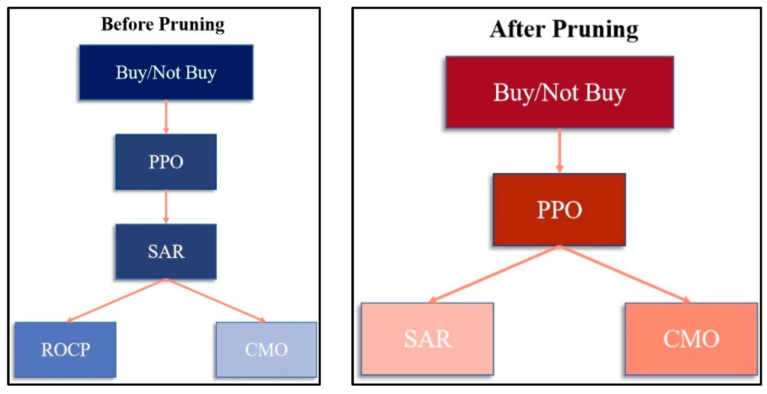
• Construction of quantitative evaluation model of decision tree.

The process of constructing the comprehensive investment appraisal coefficient (CIAC) model was as follows: first, wise buy and sell points were selected based on real data based on the principle of buying low and selling high, and the behavior of the indicator response at each point on that day was calculated based on the predicted data and abstracted as the CIAC coefficient, and 1/0 was specified as the yes/no signal, respectively, as summarized below:

Table 2. Data set of economic indicators characteristics.

CMO	APO	ROCP	SAR	PPO	B/NB	CMO	APO	ROCP	SAR	PPO	S/NS
1	0	0	0	0	0	0	0	0	0	0	0
0	1	1	0	0	0	0	0	1	1	0	0
1	1	0	1	1	1	1	0	1	0	0	1
1	1	0	0	1	1	1	1	1	0	1	1
…	…	…	…	…	…	…	…	…	…	…	…
0	0	1	1	0	0	1	1	1	0	0	1
0	1	1	0	0	1	0	0	0	0	1	0

reflects the impact factor of each indicator

Second, in order to ensure “generalization” and prevent overfitting, we chose the CART algorithm including decision tree pruning, which has the main advantage over other algorithms in that the Gini index is chosen as the feature selection method.

The Gini index is a feature selection method defined for probability distributions. Assuming that the sample has K class and the probability that the sample belongs to the K class, the Gini index of the probability distribution of that sample class can be defined as:

$$\mathrm{Gini}\left(\mathrm{P}\right)={\displaystyle \sum }_{k=1}^k{P}_k\left(1-P_k\right)=1-{\displaystyle \sum }_{k=1}^k{P}_k^2$$

(11)

For a given training set D that is the set of samples belonging to class, the Gini index of this training set can be defined as:

$$\mathrm{Gini}\left(\mathrm{D}\right)=1-{\displaystyle \sum }_{\mathrm{k}=1}^{\mathrm{k}}{\left(\frac{\left|{\mathrm{C}}_{\mathrm{k}}\right|}{\left|\mathrm{D}\right|}\right)}^2$$

(12)

If the training set is divided into and two parts according to a certain value of the feature, then the Gini index of the training set under this condition of the feature can be defined as:

$$\mathrm{Gini}\left(\mathrm{D},\mathrm{A}\right)=\frac{{\mathrm{D}}_1}{\mathrm{D}}\mathrm{Dini}\left({\mathrm{D}}_1\right)+\frac{{\mathrm{D}}_2}{\mathrm{D}}\mathrm{Dini}\left({\mathrm{D}}_2\right)$$

(13)

The Gini index of the training set indicates the uncertainty of this set, which represents the uncertainty of the training set after division. For this classification task for whether to buy stocks and whether to sell stocks, the smaller the uncertainty in the training set, the better the corresponding features are able to classify the samples.

The CART algorithm is a learning method that outputs conditional distributions of random variables given random variables, in which the generated decision trees are binary decision trees with internal nodes taking values of “true” and “false”, and the above method of node partitioning is equivalent to recursively dichotomizing each. The node partitioning method is equivalent to recursively dichotomizing each feature, dividing the feature space into a finite number of cells, and determining the predicted probability distribution over these cells. The posterior pruning of the decision tree is to select the decision tree model with the smallest loss function given the complexity determination. Given the decision tree and the regularization parameters obtained by the generative algorithm, the specific algorithm logic diagram is as follows (Figure 2).

The main nodes of our post-pruning CART classification decision tree are CMO, SAR and PPO, and the above three nodes are used as the important basis for our judgment. In Figure 3 we show the decision tree model.

CMO (Chandler momentum oscillator), one of the momentum indicators, unlike other momentum indicators oscillators such as relative strength indicator (RSI) and stochastic (KDJ), the Chandler momentum indicator uses data from both up and down days in the numerator of the calculation formula. The CMO indicator looks for extremely overbought and extremely oversold conditions with the formula:

$$\mathrm{CMO}=\frac{\left(\mathrm{Su}-\mathrm{Sd}\right)\times 100}{\left(\mathrm{Su}+\mathrm{Sd}\right)}$$

(14)

where ${\mathrm{S}}_{\mathrm{u}}$ is the sum of the difference between today’s closing price and yesterday’s closing price (up day), if the day is down, the increase value is 0. Sd is the sum of the absolute value of the difference between today’s closing price and yesterday’s closing price (down day), if the day is up, the increase value is 0.

Parabolic indicator (SAR) is also known as the stop loss point steering indicator, because the points that make up the SAR move in an arc, so it is called “parabolic steering”.

$$\mathrm{SAR}\left({\mathrm{T}}_{\mathrm{n}}\right)=\mathrm{SAR}\left({\mathrm{T}}_{\mathrm{n}-1}\right)+\mathrm{AF}\left({\mathrm{T}}_{\mathrm{n}}\right)\times \left[\mathrm{EP}\left({\mathrm{T}}_{\mathrm{n}-1}\right)-\mathrm{SAR}\left({\mathrm{T}}_{\mathrm{n}-1}\right)\right]$$

(15)

where SAR(${\mathrm{T}}_{\mathrm{n}}$) is the SAR value of the ${\mathrm{T}}_{\mathrm{n}}$ cycle and SAR (${\mathrm{T}}_{\mathrm{n}-1}$) is the value of the (${\mathrm{T}}_{\mathrm{n}-1}$)th cycle, AF is the acceleration factor (or acceleration factor) and EP is the pole price (highest or lowest price).

The percentage price oscillator (PPO) is a momentum oscillator used to measure the difference between two moving averages as a percentage of the larger moving average. the PPO reading is independent of the price level of the security and allows comparison of PPO readings across securities even if there is a large price difference; with the following formula:

$$\mathrm{PPO}=\frac{\mathrm{EMA}\left(12\right)-\mathrm{EMA}\left(26\right)}{\mathrm{EMA}\left(26\right)}\times 100$$

(16)

where EMA is the exponential moving average, and for the series defines its periodic exponential moving average up to the term as:

$${\mathrm{EMA}}_{\mathrm{N}}\left({\mathrm{x}}_{\mathrm{n}}\right)=\frac{2}{\mathrm{N}+1}{\displaystyle \sum }_{\mathrm{k}=0}^{\infty }{\left(\frac{\mathrm{N}-1}{\mathrm{N}+1}\right)}^{\mathrm{k}}{\mathrm{x}}_{\mathrm{n}-\mathrm{k}}$$

(17)

We scored the buy/sell points based on the number of times the three indicators were triggered at each point in time, with +10 points for each of the three indicators, and +20 points for CMO and PPO at the same time, resulting in a buy/sell scoring scale from 0–50 points.

3.3.2. Decision Modeling

This section will describe the process of modeling specific gold and bitcoin investment strategies. From the evaluation model, we can initially conclude that the stock buying and selling strategies can be developed by combining the CMO, PPO and SAR indicators to rate the characteristics of the stocks that appear then, but the degree to which the ratings of specific gold and bitcoin reach to operate to obtain the most benefit has not been determined. To simplify the study of this problem, we abstractly map the process of stock manipulation to the propagation of a “virus”, and the correspondence is shown in the following

Table 3. Market trading-virus transmission comparison table.

Market Transactions	Viral Transmission
Buy	Illness
Sell out	Healing
Rating	Severity
Get profit	The cost of healing
Investment amount	Accumulation of toxins

.

When the threshold is initially reached when sick (corresponding to stock purchase) and cured when the threshold is reached for the second time (corresponding to the sale of stocks), bitcoin and gold stocks correspond to factors leading to sickness that can only be treated in two hospitals A and B, respectively (corresponding to the choice of bitcoin and gold stocks). A meta-automaton simulation survival game was built based on the above mapping to study the impact of the buying and selling strategies formulated by the stock scoring thresholds on the final profit from the perspective of virus propagation and cure.

Next, a function space was constructed using the predicted data of daily bitcoin and gold stock changes, where, represents the bitcoin and gold stock ticket prices oI day i, respectively, from which the virus severity state function is defined as follows.

$${\mathrm{S}}_{\mathrm{i}}=\{\begin{array}{cc}0,\hfill & \hfill \mathrm{CMO},\mathrm{PPO},\mathrm{SAR} \mathrm{all} \mathrm{are}0\\ 10,\hfill & \hfill \mathrm{CMO},\mathrm{PPO},\mathrm{SAR} \mathrm{have} \mathrm{one} \mathrm{for} 1\\ 20,\hfill & \hfill \mathrm{CMO},\mathrm{PPO},\mathrm{SAR} \mathrm{have} \mathrm{two} \mathrm{for} 1\mathrm{and} \mathrm{CMO},\mathrm{SAR} \mathrm{not} \mathrm{both} \mathrm{for} 1\\ 30,\hfill & \hfill \mathrm{Equilibrium} \mathrm{decomposition} \mathrm{line}\\ 40,\hfill & \hfill \mathrm{CMO},\mathrm{SAR} \mathrm{both} \mathrm{are} 1\\ 50,\hfill & \hfill \mathrm{CMO},\mathrm{PPO},\mathrm{SAR} \mathrm{all} \mathrm{are} 1\end{array}$$

(18)

The buy–sell thresholds for gold and bitcoin are defined as ${\mathrm{G}}_{\mathrm{buy}}$, ${\mathrm{G}}_{\mathrm{sale}}$, ${\mathrm{B}}_{\mathrm{buy}}$ and ${\mathrm{B}}_{\mathrm{sale}}$, respectively, and in each round of virus propagation simulation these four thresholds are chosen randomly to select one of the six, 0, 10, 20, 30, 40 and 50, until the end of the current round of propagation. If one of gold and bitcoin reaches the threshold It the i time point, the state is changed to the sick state, and if the severity of the virus corresponding to the sick state reaches the threshold at the j (j > i) time point the state is changed to the cured state and the accumulated toxin produced after this cure is calculated with the following equation.

$${\mathrm{D}}_{\mathrm{t}+1}=\frac{{\mathsf{\alpha }}^2\times {\mathrm{D}}_{\mathrm{t}}\times {\mathrm{M}}_{\mathrm{j}}}{{\mathrm{M}}_{\mathrm{i}}}$$

(19)

The cost of the cure resulting from the above result update is:

$${\mathrm{money}}_{\mathrm{t}+1}=\frac{{\mathsf{\alpha }}^2\times {\mathrm{D}}_{\mathrm{t}}\times {\mathrm{M}}_{\mathrm{j}}}{{\mathrm{M}}_{\mathrm{i}}}-{\mathrm{D}}_{\mathrm{t}}$$

(20)

The state of the virus and the accumulated toxin were continuously propagated in the function space as time advances. After 1296 simulations of the virus propagating and curing in the complete time period, we concluded that the maximum value that the final toxin accumulated by the virus can reach is 36,798.49157 when the initial toxin is 1000, and the two viruses complete the disease curing process 10 times and 5 times, respectively, corresponding to the threshold values are (20, 20) and (50, 50), respectively.

4. Results

In this section, we use ConvLSTM deep learning method to construct an economic prediction model by obtaining the data of closing prices of gold and bitcoin in US dollars on the specified date and build an investment decision model by decision tree and contagion model. Firstly, the data set was preprocessed and divided into training and testing sets to train and predict the experimental results under this model. Secondly, the economic impact factors with higher weights were selected through the decision tree, and the complete strategy model was constructed by combining the features of the contagion model. Plus, we took USD 1000 as the initial capital to simulate the decision. Finally, the results are analyzed to decide the optimal trading strategy. The feasibility and advantages of the prediction model are also verified. To provide the model basis for subsequent application research.

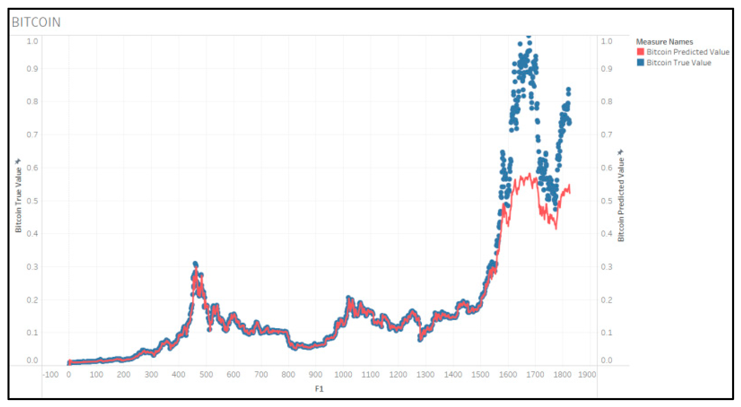
4.1. CONVLSTM Model Results Analysis

We first used 80% of the data as the training set and 20% of the data as the test set, using Adam as the optimizer. The loss function was MSE to train the CONVLSTM network model and keep tuning the parameters. The optimal network model was selected using the Euclidean distance matrix and the heat map was plotted. As shown in Figure 4 and Figure 5. The trained model was finally saved, and the model was used to predict the bitcoin price.

The final data for the daily closing price forecasts for each of gold and bitcoin were derived and analyzed by comparing the true values with our forecasts. To see the forecast trend more clearly, a special biaxial chart was drawn, see Figure 6 and Figure 7.

Where the red line indicates the predicted value of the closing price, and the blue dot represents the true closing price. By comparing the red line and the blue dot in the graph, we can see that the new forecasting model perfectly avoids the problem of forecasting lag, which is also reflected in our control model. The results of this experiment show that the predicted values obtained using the ConvLSTM deep learning method are in line with the trend of the true value. Moreover, the data in Bitcoin for a period of time shows a sudden spike, the situation is due to some sudden social factors. Obviously, this is an extreme case, but the predicted that values obtained by the model are still in line with the trend of the real values.

Figure 8 and Figure 9 show the upward trend of bitcoin and gold. It is obvious that the price difference of the experimental prediction results basically matches the upward trend in Figure 8 and Figure 9. The lowest point in Figure 9 coincides with the predicted value in Figure 7 being significantly lower than the true value. This precisely reflects the fact that the sudden change in bitcoin’s rise at this moment is unpredictable, and therefore it can be determined that the predictions derived from the experiment are accurate.

4.2. Analysis of the Results of the Control Model

In order to provide a control group for the above forecasting model and to improve the accuracy of the forecasts, therefore, we built a new model. The moving average-based support vector machine economic forecasting model allows high dimensional expansion of sample data by support vector machine. In principle, SVM uses nonlinear feature mapping to map low-dimensional features to high-dimensional ones and computes the inner product between high-dimensional features directly through kernel trick to avoid explicitly computing nonlinear feature mapping. Then linear classification is conducted in the high-dimensional feature space. The nonlinear mapping is represented by Equation (21) and it corresponds to a kernel function such that.

$$<\mathsf{\phi }\left(\mathrm{x}\right)+\mathsf{\phi }\left(\mathrm{y}\right)\ge \mathrm{k}\left(\mathrm{x}, \mathrm{y}\right)$$

(21)

Moving averages are averages of securities prices (indices) over a certain period of time, and the averages were connected at different times to form a forecast curve. It is a technical indicator used to observe the trend of securities price movements. Its calculation is as follows:

$$\mathrm{N}-\mathrm{Day} \mathrm{Moving} \mathrm{Average}=\frac{\mathrm{Sum} \mathrm{of} \mathrm{N}-\mathrm{day} \mathrm{closing} \mathrm{prices}}{\mathrm{N}}$$

(22)

The behavior of moving averages was added to the support vector machine forecasting by adjusting it. This combination improves the accuracy of the predicted values, and, also, provides economic support for the support vector machine prediction model.

In this paper, we take the moving average as 10 days and combine it with the prediction model developed, which in turn leads to Figure 10, Figure 11 and Figure 12. Bulleted lists look like this:

From Figure 12 we can roughly observe the predicted value curve compared to the true value curve. In the case of gold, for example, the forecast value has a serious lag factor. This produces a significant error in the forecast value, which can be reasonably explained by the Hurst exponent test. Thus, while confirming the difficulty of achieving the ultimate goal with short-term forecasts, it also reinforces the reliability of the first forecasting model.

4.3. Analysis of Decision Model Results

In this section, we invest by setting an initial investment amount of USD 1000. Simulation experiments are conducted to find the optimal investment plan by using the evaluation and decision model in Section 2. The maximum return that an initial investment amount of USD 1000 can obtain on 10 September 2021, is USD 36,798.49157 for bitcoin buy–sell thresholds of 20 and 20, respectively, and gold buy–sell thresholds of 50 and 50, respectively. There are 10 bitcoin trades and 5 gold trades. We have plotted the returns of some of the trading strategies Figure 13.

Looking at the return graphs of the trading strategies, we can see that the benefits of this model are not reflected in the return amounts alone. However, from a process perspective, the timing of each simulated buy or sell is more reasonable due to the inclusion of the new economic indicators, which provide a more reasonable consideration of human emotions. Other models may bring higher returns, but they are predicted and analyzed from a long-term perspective. The introduction of the new indicators will allow the model to have an artificial emotional stimulus, allowing for a more anthropomorphic investment decision in the short-term trend. Therefore, the model and the conclusions are more in line with the general rule and more realistic.

5. Discussion

The price fluctuations of virtual currencies belong to a continuous-time random walk data, where the price at each time point is random. Only by identifying the hidden patterns connecting these price fluctuations is it possible to make reasonable predictions of prices. This paper provides a possible idea to solve the decision problem associated with such data by using a deep learning model with special gating coupled with a priori knowledge. As can be seen from the line graph of returns presented in Figure 13, the model is able to both buy quickly before the price of bitcoin rises and sell in time before it falls significantly. However, the econometric indicators used to make decisions on the predicted data were selected from five existing econometric indicators using a decision tree model, and limited experiments were not able to determine the most appropriate econometric indicators. It is also worth exploring whether the economics indicators are compatible with the hidden information extracted by the deep learning model. If the economics indicators can be incorporated into the gating layer of the deep learning model, the return and prediction accuracy of the model may be improved. Compared with other quantitative trading models, the model proposed in this paper has a stronger risk-averse ability to combine the hidden connections behind the fluctuations of long-time series data and short-time series data when making decisions. Although the decisions made at some moments can lead to losses in the short run, they are the right choice to reduce risk in the long run. After changing the initial capital, the overall buying strategy does not change significantly. However, the comparison shows that with USD 10,000 as the initial capital, the final return fluctuates considerably. This is consistent with reality, and becomes increasingly evident as the initial capital base continues to expand. The idea is expected to be able to be applied to the prevention and control of the new coronavirus: first use a deep learning model to train the data of the area since the first outbreak, then make predictions for the short-term future, and, finally, use the infection rate, mortality rate and incubation period of the virus as decision indicators to determine whether a home quarantine policy should be applied to the area.

6. Conclusions

In this paper, a quantitative trading model with decision making capability is constructed using ConvLSTM coupled with economic indicators. Using 80% of the bitcoin data published on Kaggle up to 2021 as the training set and 20% as the test set, the model was trained for 1000 convergences applying Adam as the optimizer and the MSE loss function. The results show that with USD 1000 as the starting amount, the returns are able to reach 37 times. After validation, it can be determined that ConvLSTM can effectively extract the complex hidden spatial information of bitcoin price data, and the economic indicators for buying and selling decisions can effectively reduce risk and increase returns. In this paper, the idea of using deep learning models for forecasting and establishing a circular exit mechanism using a priori knowledge of related fields provides an effective solution for short-term forecasting of other long time series data affected by complex factors. (In the “Computer Science and Symmetry” section of the journal Symmetry, we find its commitment to the fields of big data, machine learning and artificial intelligence, which are compatible with the models we build for deep learning. Additionally, our topic has some new breakthroughs in deep learning).

References

1. Nelson, B.K. Time series analysis using autoregressive integrated moving average (ARIMA) models. Acad. Emerg. Med. 1998, 5, 739–744. [Google Scholar] [CrossRef] [PubMed]
2. Ullrich, T. On the Autoregressive Time Series Model Using Real and Complex Analysis. Forecasting 2021, 3, 716–728. [Google Scholar] [CrossRef]
3. Baragona, R.; Battaglia, F.; Cucina, D. Periodic autoregressive models for time series with integrated seasonality. J. Stat. Comput. Simul. 2021, 91, 694–712. [Google Scholar] [CrossRef]
4. Andriyanov, N.; Korovin, D. Analysis of the Restrictive Measures Impact on the Disease Spread. In Proceedings of the 2021 International Conference on Information Technology and Nanotechnology (ITNT), Samara, Russia, 20–24 September 2021; pp. 1–6. [Google Scholar]
5. Zhang, G.P. Time series forecasting using a hybrid ARIMA and neural network model. Neurocomputing 2003, 50, 159–175. [Google Scholar] [CrossRef]
6. Dunis, C.L.; Nathani, A. Quantitative trading of gold and silver using nonlinear models. Neural Netw. World 2007, 17, 93. [Google Scholar]
7. Pascanu, R.; Mikolov, T.; Bengio, Y. On the difficulty of training recurrent neural networks. In International Conference on Machine Learning; PMLR: 2013. In Proceedings of the International Conference on Machine Learning, Atlanta, GA, USA, 16–21 June 2013; PMLR: Cambridge, MA, USA, 2013. [Google Scholar]
8. Hochreiter, S. The vanishing gradient problem during learning recurrent neural nets and problem solutions. Int. J. Uncertain. Fuzziness Knowl.-Based Syst. 1998, 6, 107–116. [Google Scholar] [CrossRef]
9. Hochreiter, S.; Schmidhuber, J. Long short-term memory. Neural Comput. 1997, 9, 1735–1780. [Google Scholar] [CrossRef] [PubMed]
10. Lukáš, P.; Taisei, K. Volatility analysis of bitcoin price time series. Quant. Financ. Econ. 2017, 1, 474–485. [Google Scholar]
11. McNally, S.; Roche, J.; Caton, S. Predicting the Price of Bitcoin Using Machine Learning. In Proceedings of the 2018 26th Euromicro International Conference on Parallel, Distributed and Network-Based Processing (PDP), Cambridge, UK, 21–23 March 2018; pp. 339–343. [Google Scholar]
12. Siami-Namini, S.; Namin, A.S. Forecasting economics and financial time series: ARIMA vs. LSTM. arXiv 2018, arXiv:1803.06386. [Google Scholar]
13. Wang, L.; Zeng, Y.; Chen, T. Back propagation neural network with adaptive differential evolution algorithm for time series forecasting. Expert Syst. Appl. 2015, 42, 855–863. [Google Scholar] [CrossRef]
14. Yin, W.; Kann, K.; Yu, M.; Schütze, H. Comparative study of CNN and RNN for natural language processing. arXiv 2017, arXiv:1702.01923. [Google Scholar]
15. Srivastava, N.; Hinton, G.; Krizhevsky, A.; Sutskever, I.; Salakhutdinov, R. Dropout: A simple way to prevent neural networks from overfitting. J. Mach. Learn. Res. 2014, 15, 1929–1958. [Google Scholar]
16. Shi, X.; Chen, Z.; Wang, H.; Yeung, D.-Y.; Wong, W.-K.; Woo, W.-C. Convolutional LSTM network: A machine learning approach for precipitation nowcasting. Adv. Neural Inf. Process. Syst. 2015, 28. [Google Scholar]
Figure 1. Logical mind map.
Symmetry 14 01896 g001
Figure 2. Post-pruning CART classification decision tree algorithm.
Symmetry 14 01896 g002
Figure 3. Decision tree model.
Symmetry 14 01896 g003
Figure 4. Bitcoin heat map.
Symmetry 14 01896 g004
Figure 5. Gold heat map.
Symmetry 14 01896 g005
Figure 6. Gold daily price forecast chart.
Symmetry 14 01896 g006
Figure 7. Bitcoin daily price forecast chart.
Symmetry 14 01896 g007
Figure 8. Gold up and down trend.
Symmetry 14 01896 g008
Figure 9. Bitcoin up and down trend.
Symmetry 14 01896 g009
Figure 10. Bitcoin forecast chart 2.
Symmetry 14 01896 g010
Figure 11. Gold forecast chart 2.
Symmetry 14 01896 g011
Figure 12. Partial forecast curve.
Symmetry 14 01896 g012
Figure 13. Final strategy comparison chart (The red box is the optimal solution).
Symmetry 14 01896 g013