Article

Hermite–Hadamard-Type Inequalities Involving Harmonically Convex Function via the Atangana–Baleanu Fractional Integral Operator

by
Muhammad Amer Latif
1,
Humaira Kalsoom
2,* and
Muhammad Zainul Abidin
2,*
1
Department of Basic Sciences, King Faisal University, Hofuf 31982, Saudi Arabia
2
Department of Mathematics, Zhejiang Normal University, Jinhua 321004, China
*
Authors to whom correspondence should be addressed.
Symmetry 2022, 14(9), 1774; https://doi.org/10.3390/sym14091774
Submission received: 31 May 2022 / Revised: 24 June 2022 / Accepted: 2 July 2022 / Published: 25 August 2022
(This article belongs to the Topic Fractional Calculus: Theory and Applications)

Abstract

:
Fractional integrals and inequalities have recently become quite popular and have been the prime consideration for many studies. The results of many different types of inequalities have been studied by launching innovative analytical techniques and applications. These Hermite–Hadamard inequalities are discovered in this study using Atangana–Baleanu integral operators, which provide both practical and powerful results. In this paper, a symmetric study of integral inequalities of Hermite–Hadamard type is provided based on an identity proved for Atangana–Baleanu integral operators and using functions whose absolute value of the second derivative is harmonic convex. The proven Hermite–Hadamard-type inequalities have been observed to be valid for a choice of any harmonic convex function with the help of examples. Moreover, fractional inequalities and their solutions are applied in many symmetrical domains.

1. Introduction

Integral inequalities are fundamental to our comprehension of the cosmos, and there are a great deal of straightforward methods available for determining the uniqueness and existence of linear and nonlinear differential equations in which symmetry is a significant factor. Convex functions are of great interest to researchers in many applied fields, such as convex programming, because they are extremely important for the theory of inequality in a wide range of applications. Convex functions are also of great interest to researchers in many theoretical fields, such as probability theory. It is good to start by recognizing this class of function.
Definition 1.
A function f : I R R is convex if for all ϖ 1 , ϖ 2 I , the inequality
f t ϖ 1 + 1 t ϖ 2 t f ϖ 1 + 1 t f ϖ 2
holds. A function f : I R is concave in which the inequality (1) holds in the opposite direction.
In this case, convex functions play an important role in many areas of mathematics. They are especially important in the study of optimization problems where they are distinguished by a number of convenient properties. Moreover, convex functions are used to create a historical inequality, which is a kind of beautiful inequality in which one has the ability to express the lower and higher limits as arithmetic means. It is critical in numerical integration to understand the inequality described here because it is used in error estimation formulas such as the trapezoidal and midpoint formulas (for more details, see [1,2,3,4,5,6,7]):
f ϖ 1 + ϖ 2 2 1 ϖ 2 ϖ 1 ϖ 1 ϖ 2 f x d x f ϖ 1 + f ϖ 2 2 ,
where the function f : I R is convex on I and f L 1 ϖ 1 , ϖ 2 .
One of the generalizations of the convex functions is the harmonic convex functions, which are defined as follows:
Definition 2
([7]). A function f : I R 0 R is harmonic convex if for all ϖ 1 , ϖ 2 I , the inequality
f ϖ 1 ϖ 2 t ϖ 2 + 1 t ϖ 1 t f ϖ 1 + 1 t f ϖ 2
holds. A function f : I R 0 R is harmonic concave in which the inequality (3) holds in the opposite direction. For more details about harmonic convex functions, please see [8,9,10,11].
A variant of the Hermite–Hadamard inequality (2) for harmonic convex functions was proved by İşcan [7].
Theorem 1
([7]). Let f : I R 0 R be a harmonically convex function and ϖ 1 , ϖ 2 I with ϖ 1 < ϖ 2 . If f L [ ϖ 1 , ϖ 2 ] ; then, the following inequalities hold:
f 2 ϖ 1 ϖ 2 ϖ 1 + ϖ 2 ϖ 1 ϖ 2 ϖ 2 ϖ 1 ϖ 1 ϖ 2 f x x 2 d x f ϖ 1 + f ϖ 2 2 .
Convexity and integral inequality are topics that are explored in several works. This type of research is oriented on examining the properties of Hadamard, Bullen, Ostrowski, and Simpson-type inequalities, which can be discovered in the results of Static Neural Networks, as well as the properties of other types of inequalities. Every study introduced a new strategy and opened new application opportunities for the literature. The articles [12,13,14,15,16,17,18] offer additional information on convexity and integral inequalities in various directions:
Fractional integral inequalities benefit from the properties and definition of convexity, and it has recently become an immensely important topic of research. A newly emerged field in applied mathematics, called fractional analysis, is concerned with finding answers to open problems involving fractional-order derivatives. After discovering this solution, mathematicians have found themselves embarking on brand-new lines of inquiry due to how much research interest there has been in the field for decades. In addition to the Riemann–Liouville fractional integrals, fractional integral operators and fractional derivatives have become major parts of applied mathematics and applied sciences. Solutions to real-world problems are proposed by fractional integral and derivative operators, which also improve the relationship between mathematics and other disciplines when it comes to applications. Those interested in learning more about fractional integral and derivative operators should begin with the articles [19,20,21,22,23,24,25,26,27,28,29,30,31,32,33,34,35,36,37,38,39,40,41,42,43,44,45,46]. An important concept, not long ago, that has emerged is the Caputo–Fabrizio integral operator, which was established in the last few years. This is how it is defined:
Definition 3
([47]). Let f H 1 0 , ϖ 2 , ϖ 1 < ϖ 2 , α 0 , 1 ; then, the definition of the new Caputo fractional derivative is:
C F D α f x = M α 1 α ϖ 1 x f t exp α x t 1 α d t ,
such that M α is a normalization function.
The Caputo–Fabrizio fractional integral formula is:
Definition 4
([21]). Let f H 1 0 , ϖ 2 , ϖ 1 < ϖ 2 , α 0 , 1 So, the left and right sides of the Caputo–Fabrizio fractional integral are:
ϖ 1 C F I α f x = 1 α B α f x + α B α ϖ 1 x f t d t
and
C F I ϖ 2 α f x = 1 α B α f x + α B α x ϖ 2 f t d t ,
where B α is normalization function.
Atangana–Baleanu [5] has found a solution to the problem of the Caputo–Fabrizio operator not being reduced to the original function in a special case, despite the fact that the operator is an effective tool in the solution of many systems of differential equations. The features of the Caputo–Fabrizio operator are present in the normalization function.
The power law is included in the kernel of some fractional order derivative and integral operators as well as some integral operators. Nature does not usually exhibit power law behavior. This novel derivative and integral operator incorporates the Mittag–Leffler function [48]. The Mittag–Leffler function is required to model nature. This improved the Atangana–Baleanu operator and piqued researchers’ interest. That the work uses the Atangana–Baleanu operator for Hermite–Hadamard inequalities is unusual. When the parameter is set to zero, the Atangana–Baleanu original function can be derived and compared to the Caputo–Fabrizio results.
Definition 5
([5]). Let f H 1 0 , ϖ 2 , ϖ 1 < ϖ 2 , α 0 , 1 ; then, the definition of the new fractional derivative is given below
ϖ 1 A B C D x α f x = B α 1 α ϖ 1 x f t E α α x t α 1 α d t .
Definition 6
([5]). Let f H 1 0 , ϖ 2 , ϖ 1 < ϖ 2 , α 0 , 1 ; then, the definition of the new fractional derivative is given below:
ϖ 1 A B C D x α f x = B α 1 α d d x ϖ 1 x f t E α α x t α 1 α d t .
Equations (7) and (8) have a non-local kernel. In addition, in (8), as a result, the constant function returns to zero. The following is the definition of the associated integral operator for the Atangana–Baleanu fractional derivative:
Definition 7
([5]). The new fractional derivative with a non-local kernel of a function is associated with the fractional integral f H 1 0 , ϖ 2 as defined:
ϖ 1 A B I α f x = 1 α B α f x + α B α Γ α ϖ 1 x f t x t α 1 d t ,
where ϖ 1 < ϖ 2 , α 0 , 1 .
The authors of [22] described the integral operator’s right-hand side as follows:
A B I ϖ 2 α f x = 1 α B α f x + α B α Γ α x ϖ 2 f t t x α 1 d t ,
where ϖ 1 < ϖ 2 , α 0 , 1 .
Mathematical concepts can be thought of as having practical and theoretical significance. Furthermore, among the qualities that make the concepts strong are that they solve a deficiency, provide a new workplace orientation and are more functional than existing concepts. The significance and power of fractional analysis investigations can be better understood when seen from this perspective. The literature acknowledges an operator whose definition and properties are expressed because it is popular in the domain of usage and invention. The Atangana–Baleanu derivative and related integral operator have proven particularly useful. Although many investigations on this unusual operator have been completed in a short time, the results demonstrate that the operator is efficient and valuable. We advise academics to undertake their own independent research to learn more about new directions and trends in fractional calculus.
In [37], Set et al. proved new Hermite–Hadamard-type inequalities, which are for functions whose absolute value of the second derivatives are convex, using Atangana–Baleanu integral operators. Set et al. [37] used Atangana–Baleanu operators to generate new and general Hermite–Hadamard-type inequalities and to make discoveries that better explain physical phenomena in terms of the kernel structure and characteristics of the operator. Selecting α equal to 1 will give a different classical Hermite–Hadamard inequality. In the first place, an identity using Atangana–Baleanu was obtained by various integration techniques, and on the other hand, a modification is made in this identity, and hence, a new set of integral inequalities was proved.
During the course of the last three decades, the study of mathematical inequalities that make use of convex functions has been recognized as a prominent field of research. The researchers are looking for new generalizations of convex functions, and as a consequence, new findings are being added to the theory of inequality as a result of their efforts. Within the scope of the present investigation, we have made use of harmonic convex functions in order to generalize a number of findings that are valid for convex functions. The study initiated by Set et al. [
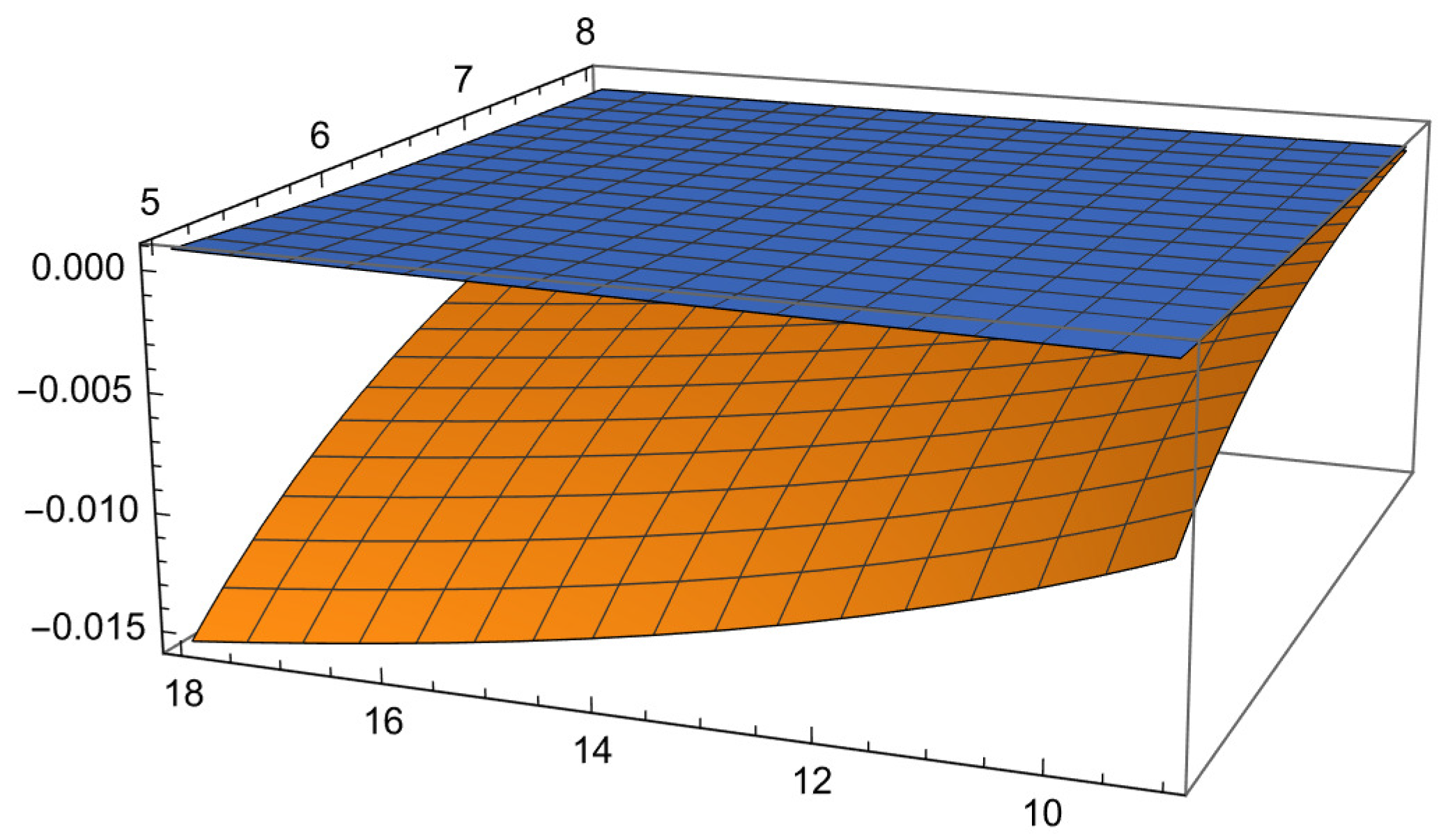
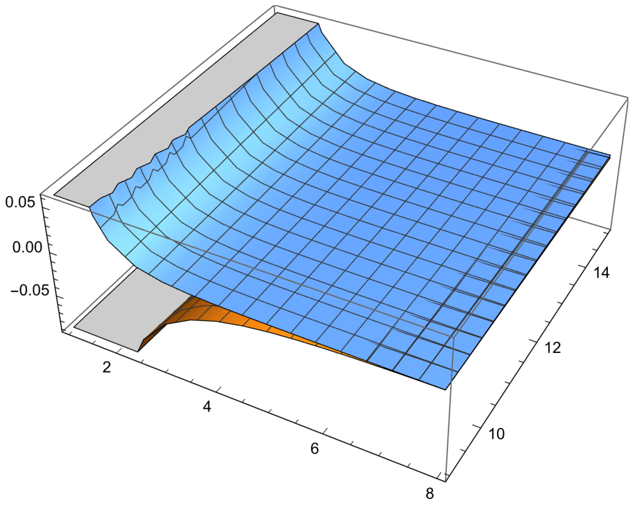
37] provided a sound motivation for us to conduct similar research toward harmonic convex functions. We first set up an identity using an Atangana–Baleanu integral operator as well as the properties of harmonic convexity and the use of several integration techniques to obtain new results of Hermite–Hadamard type. We also try to make amendments in the main identity and applications of a number of known famous integral inequalities to prove a new variety of integral inequalities of Hermite–Hadamard type in the next section, with the property that the derivative of the function in absolute value having certain powers is harmonic convex. The proven Hermite–Hadamard-type inequalities have been observed to be valid for a choice of any harmonic convex function with the help of examples. Moreover, the Figure 1 shows the validity of Theorem 7 and Figure 2 shows the validity of Theorem 3.

2. Main Results

The following lemma will be used to show the Hermite–Hadamard-type integral inequalities for the first time in the literature of inequalities theory. The following result is actually a consequence of the sum of two symmetric integrals and is useful to obtain our results.
Lemma 1.
Let f : I 0 , R be differentiable mapping on I (the interior of I) and ϖ 1 , ϖ 2 I with ϖ 1 < ϖ 2 . Then, the Atangana–Baleanu identity holds for fractional integral operators
Φ f h 1 ϖ 1 A B I 1 x α , 1 ϖ 2 A B I 1 x α : = x ϖ 1 x ϖ 1 α + 1 B α Γ α α 1 x f ϖ 1 + ϖ 1 x ϖ 1 2 f ϖ 1 f ϖ 1 ϖ 1 x 2 x ϖ 1 ϖ 2 x ϖ 2 x α + 1 B α Γ α α 1 x f ϖ 2 + ϖ 2 ϖ 2 x 2 f ϖ 2 f ϖ 2 ϖ 2 x 2 ϖ 2 x + α 1 ϖ 1 2 x 2 1 ϖ 1 A B I 1 x α f h x 1 α B α f h x 2 α B α + 1 ϖ 1 2 x 3 α + 1 B α × 1 ϖ 1 A B I 1 x α + 1 h x 2 f h x + α B α + 1 h x 2 f h x
+ α 1 ϖ 2 2 x 2 1 ϖ 2 A B I 1 x α f h x 1 α B α f h x + 2 α B α + 1 ϖ 2 2 x 3 α + 1 B α
× 1 ϖ 2 A B I 1 x α + 1 h x 2 f h x + α B α + 1 h x 2 f h x 2 ϖ 1 2 x 3 1 ϖ 1 A B I 1 x α h x f h x 1 α B α h x f h x + 2 ϖ 2 2 x 3 1 ϖ 2 A B I 1 x α h x f h x 1 α B α h x f h x = ϖ 2 x ϖ 2 x B α Γ α ϖ 2 x ϖ 2 x α + 1 0 1 t α + 1 t x + 1 t ϖ 2 4 f ϖ 2 x t x + 1 t ϖ 2 d t + ϖ 1 x x ϖ 1 B α Γ α x ϖ 1 x ϖ 1 α + 1 0 1 1 t α + 1 t ϖ 1 + 1 t x 4 f ϖ 1 x t ϖ 1 + 1 t x d t .
where h w = 1 w , w 1 ϖ 2 , 1 ϖ 1 , x ϖ 1 , ϖ 2 and α 0 , 1 .
Proof. 
We observe by integration by parts that
1 B α Γ α 0 1 1 t α t ϖ 1 + 1 t x 2 f ϖ 1 x t ϖ 1 + 1 t x d t = 1 B α Γ α × 1 α + 1 f ϖ 1 x 2 + 0 1 1 t α + 1 α + 1 ϖ 1 x x ϖ 1 t ϖ 1 + 1 t x 4 f ϖ 1 x t ϖ 1 + 1 t x d t + 0 1 1 t α + 1 α + 1 2 x ϖ 1 t ϖ 1 + 1 t x 3 f ϖ 1 x t ϖ 1 + 1 t x d t .
From (12), we obtain
α 1 B α Γ α 0 1 1 t α t ϖ 1 + 1 t x 2 f ϖ 1 x t ϖ 1 + 1 t x d t + 2 ϖ 1 B α Γ α 0 1 1 t α t ϖ 1 + 1 t x 3 f ϖ 1 x t x + 1 t ϖ 1 d t = 1 B α Γ α × f ϖ 1 x 2 + ϖ 1 x x ϖ 1 0 1 1 t α + 1 t ϖ 1 + 1 t x 4 f ϖ 1 x t ϖ 1 + 1 t x d t .
By using the definition of Atangana–Baleanu fractional derivative, we observe that the following equalities hold
α 1 B α Γ α 0 1 1 t α t ϖ 1 + 1 t x 2 f ϖ 1 x t ϖ 1 + 1 t x d t = α 1 B α Γ α ϖ 1 x x ϖ 1 0 1 1 t α d f ϖ 1 x t ϖ 1 + 1 t x = α 1 f ϖ 1 B α Γ α ϖ 1 x x ϖ 1 + α 1 ϖ 1 x x ϖ 1 ϖ 1 x x ϖ 1 α α B α Γ α 1 x 1 ϖ 1 w 1 x α 1 f 1 w d w = α 1 f ϖ 1 B α Γ α ϖ 1 x x ϖ 1 + α 1 ϖ 1 x x ϖ 1 ϖ 1 x x ϖ 1 α × 1 ϖ 1 A B I 1 x α f h x 1 α B α f h x
and
2 ϖ 1 B α Γ α 0 1 1 t α t ϖ 1 + 1 t x 3 f ϖ 1 x t ϖ 1 + 1 t x d t = 2 x x ϖ 1 B α Γ α 0 1 1 t α t ϖ 1 + 1 t x d f ϖ 1 x t ϖ 1 + 1 t x = 2 f ϖ 1 x 2 x ϖ 1 B α Γ α 2 α α x B α Γ α 0 1 1 t α t ϖ 1 + 1 t x 2 f ϖ 1 x t ϖ 1 + 1 t x d t + 2 α x 2 x ϖ 1 B α Γ α 0 1 1 t α 1 t ϖ 1 + 1 t x f ϖ 1 x t ϖ 1 + 1 t x d t = 2 f ϖ 1 x 2 x ϖ 1 B α Γ α 2 ϖ 1 x x ϖ 1 α + 1 B α + 1 ϖ 1 2 x 3 α + 1 B α × 1 ϖ 1 A B I 1 x α + 1 h x 2 f h x + α B α + 1 h x 2 f h x + 2 ϖ 1 x x ϖ 1 α ϖ 1 x 2 x ϖ 1 1 ϖ 1 A B I 1 x α h x f h x 1 α B α h x f h x .
By applying (14) and (15) in (13), we obtain
x ϖ 1 x ϖ 1 α + 1 B α Γ α α 1 x f ϖ 1 + 2 ϖ 1 x ϖ 1 f ϖ 1 ϖ 1 x ϖ 1 f ϖ 1 ϖ 1 x 2 x ϖ 1 + α 1 ϖ 1 2 x 2 1 ϖ 1 A B I 1 x α f h x 1 α B α f h x 2 B α + 1 ϖ 1 2 x 3 α + 1 B α × 1 ϖ 1 A B I 1 x α + 1 h x 2 f h x + α B α + 1 h x 2 f h x + 2 ϖ 1 2 x 3 1 ϖ 1 A B I 1 x α h x f h x 1 α B α h x f h x = ϖ 1 x x ϖ 1 B α Γ α x ϖ 1 x ϖ 1 α + 1 0 1 1 t α + 1 t ϖ 1 + 1 t x 4 f ϖ 1 x t ϖ 1 + 1 t x d t .
Now, we consider the integral
1 B α Γ α 0 1 t α t x + 1 t ϖ 2 2 f ϖ 2 x t x + 1 t ϖ 2 d t = f ϖ 2 x 2 α + 1 B α Γ α 1 B α Γ α 0 1 t α + 1 α + 1 ϖ 2 x ϖ 2 x t x + 1 t ϖ 2 4 f ϖ 2 x t x + 1 t ϖ 2 d t 1 B α Γ α 0 1 t α + 1 α + 1 2 ϖ 2 x t x + 1 t ϖ 2 3 f ϖ 2 x t x + 1 t ϖ 2 d t .
which gives
α 1 B α Γ α 0 1 t α t x + 1 t ϖ 2 2 f ϖ 2 x t x + 1 t ϖ 2 d t + 2 ϖ 2 B α Γ α 0 1 t α t x + 1 t ϖ 2 3 f ϖ 2 x t x + 1 t ϖ 2 d t = f ϖ 2 x 2 B α Γ α ϖ 2 x ϖ 2 x B α Γ α 0 1 t α + 1 t x + 1 t ϖ 2 4 f ϖ 2 x t x + 1 t ϖ 2 d t .
It is easy to see that
α 1 B α Γ α 0 1 t α t x + 1 t ϖ 2 2 f ϖ 2 x t x + 1 t ϖ 2 d t = α 1 f ϖ 2 ϖ 2 x ϖ 2 x B α Γ α α 1 ϖ 2 x ϖ 2 x α ϖ 2 x ϖ 2 x × 1 ϖ 2 A B I 1 x α f h x 1 α B α f h x
and
2 ϖ 2 B α Γ α 0 1 t α t x + 1 t ϖ 2 3 f ϖ 2 x t x + 1 t ϖ 2 d t = 2 f ϖ 2 x 2 B α Γ α 2 ϖ 2 x ϖ 2 x α ϖ 2 x 2 ϖ 2 x 1 ϖ 2 A B I 1 x α h x f h x 1 α B α h x f h x 2 ϖ 2 x ϖ 2 x α + 1 α B α + 1 ϖ 2 2 x 3 α + 1 B α × 1 ϖ 2 A B I 1 x α h x 2 f h x + α B α + 1 h x 2 f h x .
A combination of (18)–(20) gives us
ϖ 2 x ϖ 2 x α + 1 B α Γ α α 1 x f ϖ 2 + 2 ϖ 2 ϖ 2 x f ϖ 2 ϖ 2 ϖ 2 x f ϖ 2 ϖ 2 x 2 ϖ 2 x + α 1 ϖ 2 2 x 2 1 ϖ 2 A B I 1 x α f h x 1 α B α f h x + 2 α B α + 1 ϖ 2 2 x 3 α + 1 B α × 1 ϖ 2 A B I 1 x α h x 2 f h x + α B α + 1 h x 2 f h x + 2 ϖ 2 2 x 3 1 ϖ 2 A B I 1 x α h x f h x 1 α B α h x f h x = ϖ 2 x ϖ 2 x B α Γ α ϖ 2 x ϖ 2 x α + 1 0 1 t α + 1 t x + 1 t ϖ 2 4 f ϖ 2 x t x + 1 t ϖ 2 d t .
The addition of (16) and (21) gives the required result. □
We also recall some special functions which we use to give our estimates.
The Beta or the Euler integral of the first kind and hypergeometric functions are defined as
B ( α , β ) = 0 1 t α 1 ( 1 t ) β 1 d t , α , β > 0 .
2 F 1 ( α , β ; γ , z ) = 1 B ( β , γ β ) 0 1 t β 1 ( 1 t ) γ β 1 ( 1 z t ) α d t , γ > β > 0 , | z | < 1 ,
respectively, (see [35]). The regularized hypergeometric function is defined as
2 F ˜ 1 ( α , β ; γ , z ) = 2 F 1 ( α , β ; γ , z ) Γ γ ,
where Γ γ is the gamma function.
We will now be able to generalize the Hermite–Hadamard-type inequalities using the harmonic convexity. One can easily observe that there is symmetry even in the estimates of Φ f h 1 ϖ 1 A B I 1 x α , 1 ϖ 2 A B I 1 x α .
Theorem 2.
Let f : I 0 , R be differentiable mapping on I (the interior of I) and ϖ 1 , ϖ 2 I with ϖ 1 < ϖ 2 . If f L 1 ϖ 1 , ϖ 2 and f is a harmonic convex mapping on ϖ 1 , ϖ 2 , then the following inequality for Atangana–Baleanu fractional integral operators holds
Φ f h 1 ϖ 1 A B I 1 x α , 1 ϖ 2 A B I 1 x α ϖ 2 x ϖ 2 x B α Γ α ϖ 2 x ϖ 2 x α + 1 ϕ 1 ϖ 1 , ϖ 2 , α ; x f x + ϕ 2 ϖ 1 , ϖ 2 , α ; x f ϖ 2 + ϖ 1 x x ϖ 1 B α Γ α x ϖ 1 x ϖ 1 α + 1 ϕ 3 ϖ 1 , ϖ 2 , α ; x f ϖ 1 + ϕ 4 ϖ 1 , ϖ 2 , α ; x f x ,
where
ϕ 1 ϖ 1 , ϖ 2 , α ; x = ϖ 2 ( ϖ 2 2 α x ) 6 ϖ 2 4 x 2 + α α 2 + 3 α + 2 2 F 1 1 , α + 3 ; α + 4 ; 1 x ϖ 2 6 ϖ 2 4 α + 3 α α 2 1 2 F 1 1 , α + 2 ; α + 3 ; 1 x ϖ 2 6 ϖ 2 4 α + 2 ,
ϕ 2 ϖ 1 , ϖ 2 , α ; x = ϖ 2 2 ϖ 2 2 α ϖ 2 x + α ( α + 1 ) x 2 6 ϖ 2 4 x 3 α ( α + 1 ) ( α + 2 ) Γ ( α + 3 ) 2 F ˜ 1 1 , α + 3 ; α + 4 ; 1 x ϖ 2 6 ϖ 2 4 ,
ϕ 3 ϖ 1 , ϖ 2 , α ; x = 2 ϖ 1 2 + α ( α + 1 ) x 2 α ϖ 1 x 6 ϖ 1 3 x 3 α ( α + 1 ) ( α + 2 ) Γ ( α + 3 ) 2 F ˜ 1 1 , 1 ; α + 4 ; 1 ϖ 1 x 6 ϖ 1 3 x ,
ϕ 4 ϖ 1 , ϖ 2 , α ; x = ϖ 1 2 2 α ϖ 1 x α + 2 α α 2 1 x 2 6 α + 2 ϖ 1 4 x 2 + α ( α + 1 ) Γ ( α + 3 ) ( 3 ϖ 1 + ( α 1 ) x ) 2 F ˜ 1 1 , 1 ; α + 4 ; 1 ϖ 1 x 6 ϖ 1 4 x ,
x ϖ 1 , ϖ 2 , α 0 , 1 , q > 1 , B α and Γ α are the normalization and gamma function, respectively.
Proof. 
According to (11) of Lemma 1, we obtain
Φ f h 1 ϖ 1 A B I 1 x α , 1 ϖ 2 A B I 1 x α ϖ 2 x ϖ 2 x B α Γ α ϖ 2 x ϖ 2 x α + 1 0 1 t α + 1 t x + 1 t ϖ 2 4 f ϖ 2 x t x + 1 t ϖ 2 d t + ϖ 1 x x ϖ 1 B α Γ α x ϖ 1 x ϖ 1 α + 1 0 1 1 t α + 1 t ϖ 1 + 1 t x 4 f ϖ 1 x t ϖ 1 + 1 t x d t .
Since f is a harmonic convex mapping on ϖ 1 , ϖ 2 , we obtain
0 1 t α + 1 t x + 1 t ϖ 2 4 f ϖ 2 x t x + 1 t ϖ 2 d t f x 0 1 t α + 1 1 t t x + 1 t ϖ 2 4 d t + f ϖ 2 0 1 t α + 2 t x + 1 t ϖ 2 4 d t = ϖ 2 ( ϖ 2 2 α x ) 6 ϖ 2 4 x 2 + α α 2 + 3 α + 2 2 F 1 1 , α + 3 ; α + 4 ; 1 x ϖ 2 6 ϖ 2 4 α + 3 α α 2 1 2 F 1 1 , α + 2 ; α + 3 ; 1 x ϖ 2 6 ϖ 2 4 α + 2 f x + ϖ 2 2 ϖ 2 2 α ϖ 2 x + α ( α + 1 ) x 2 6 ϖ 2 4 x 3 α ( α + 1 ) ( α + 2 ) Γ ( α + 3 ) 2 F ˜ 1 1 , α + 3 ; α + 4 ; 1 x ϖ 2 6 ϖ 2 4 f ϖ 2
and
0 1 1 t α + 1 t ϖ 1 + 1 t x 4 f ϖ 1 x t ϖ 1 + 1 t x d t f ϖ 1 2 ϖ 1 2 + α ( α + 1 ) x 2 α ϖ 1 x 6 ϖ 1 3 x 3 α ( α + 1 ) ( α + 2 ) x 2 Γ ( α + 3 ) 2 F ˜ 1 1 , 1 ; α + 4 ; 1 ϖ 1 x 6 ϖ 1 3 x 3 + f x ϖ 1 2 2 α ϖ 1 x α + 2 α α 2 1 x 2 6 α + 2 ϖ 1 4 x 2 + α ( α + 1 ) x Γ ( α + 3 ) ( 3 ϖ 1 + ( α 1 ) x ) 2 F ˜ 1 1 , 1 ; α + 4 ; 1 ϖ 1 x 6 ϖ 1 4 x 2 .
Applying (24) and (25) together in (23), we obtain the desired result. □
Corollary 1.
The substitution of x = 2 ϖ 1 ϖ 2 ϖ 1 + ϖ 2 in Theorem 2 produces the following result
Φ f h 1 ϖ 1 A B I ϖ 1 + ϖ 2 2 ϖ 1 ϖ 2 α , 1 ϖ 2 A B I ϖ 1 + ϖ 2 2 ϖ 1 ϖ 2 α 2 ϖ 1 ϖ 2 ϖ 2 ϖ 1 ϖ 1 + ϖ 2 2 B α Γ α ϖ 2 ϖ 1 2 ϖ 1 ϖ 2 α + 1 × ϖ 2 2 ϕ 1 ϖ 1 , ϖ 2 , α ; 2 ϖ 1 ϖ 2 ϖ 1 + ϖ 2 f 2 ϖ 1 ϖ 2 ϖ 1 + ϖ 2 + ϕ 1 ϖ 1 , ϖ 2 , α ; 2 ϖ 1 ϖ 2 ϖ 1 + ϖ 2 f ϖ 2 + ϖ 1 2 ϕ 3 ϖ 1 , ϖ 2 , α ; 2 ϖ 1 ϖ 2 ϖ 1 + ϖ 2 f ϖ 1 + ϕ 4 ϖ 1 , ϖ 2 , α ; 2 ϖ 1 ϖ 2 ϖ 1 + ϖ 2 f 2 ϖ 1 ϖ 2 ϖ 1 + ϖ 2 ,
where
ϕ 1 ϖ 1 , ϖ 2 , α ; 2 ϖ 1 ϖ 2 ϖ 1 + ϖ 2 = α α 2 + 3 α + 2 2 F 1 1 , α + 3 ; α + 4 ; ϖ 2 ϖ 1 ϖ 1 + ϖ 2 6 ϖ 2 4 α + 3 α α 2 1 2 F 1 1 , α + 2 ; α + 3 ; ϖ 2 ϖ 1 ϖ 1 + ϖ 2 6 ϖ 2 4 α + 2 ( ϖ 1 + ϖ 2 ) ( ϖ 1 ( 4 α 1 ) ϖ 2 ) 24 ϖ 1 2 ϖ 2 4 ,
ϕ 2 ϖ 1 , ϖ 2 , α ; 2 ϖ 1 ϖ 2 ϖ 1 + ϖ 2 = ϖ 1 + ϖ 2 ϖ 1 α ϖ 1 ϖ 2 + 2 ϖ 1 α + ϖ 1 + ϖ 2 24 ϖ 1 3 ϖ 2 4 α ( α + 1 ) ( α + 2 ) Γ ( α + 3 ) 2 F ˜ 1 1 , α + 3 ; α + 4 ; ϖ 2 ϖ 1 ϖ 1 + ϖ 2 6 ϖ 2 4 ,
ϕ 3 ϖ 1 , ϖ 2 , α ; 2 ϖ 1 ϖ 2 ϖ 1 + ϖ 2 = ( ϖ 1 + ϖ 2 ) α ϖ 2 ( ϖ 2 ϖ 1 ) + ( ϖ 1 + ϖ 2 ) 2 + 2 α 2 ϖ 2 2 24 ϖ 1 4 ϖ 2 3 α ( α + 1 ) ( α + 2 ) ( ϖ 1 + ϖ 2 ) Γ ( α + 3 ) 2 F ˜ 1 1 , 1 ; α + 4 ; ϖ 2 ϖ 1 2 ϖ 2 12 ϖ 1 4 ϖ 2 ,
ϕ 4 ϖ 1 , ϖ 2 , α ; 2 ϖ 1 ϖ 2 ϖ 1 + ϖ 2 = ϖ 1 2 + 2 ( 1 2 α ) ϖ 1 ϖ 2 α + 2 ( α ( 4 α ( α + 1 ) + 3 ) 2 ) ϖ 2 2 24 ϖ 1 4 ϖ 2 2 α + 2 + α ( α + 1 ) Γ ( α + 3 ) ( 3 ϖ 1 + 2 α ϖ 2 + ϖ 2 ) 2 F ˜ 1 1 , 1 ; α + 4 ; ϖ 2 ϖ 1 2 ϖ 2 12 ϖ 1 4 ϖ 2 ,
α 0 , 1 , B α and Γ α are the normalization and gamma function, respectively.
Theorem 3.
Let f : I 0 , R be differentiable mapping on I (the interior of I) and ϖ 1 , ϖ 2 I with ϖ 1 < ϖ 2 . If f L 1 ϖ 1 , ϖ 2 and f q is a harmonic convex mapping on ϖ 1 , ϖ 2 ; then, the following inequality for Atangana–Baleanu fractional integral operators holds
Φ f h 1 ϖ 1 A B I 1 x α , 1 ϖ 2 A B I 1 x α 1 α p + p + 1 1 p ϖ 2 x ϖ 2 x B α Γ α ϖ 2 x ϖ 2 x α + 1 × φ 1 ϖ 1 , ϖ 2 , q ; x f x q + φ 2 ϖ 1 , ϖ 2 , q ; x f ϖ 2 q 1 q + ϖ 1 x x ϖ 1 B α Γ α × x ϖ 1 x ϖ 1 α + 1 φ 3 ϖ 1 , ϖ 2 , q ; x f ϖ 1 q + φ 4 ϖ 1 , ϖ 2 , q ; x f x q 1 q ,
where
φ 1 ϖ 1 , ϖ 2 , q ; x = ϖ 2 2 4 q 2 ϖ 2 1 4 q x 4 ϖ 2 2 4 q q + x 2 4 q + 4 ϖ 2 1 4 q q x 2 ϖ 2 x 2 8 q 2 6 q + 1 ,
φ 2 ϖ 1 , ϖ 2 , q ; x = ϖ 2 4 q x 4 q x ϖ 2 4 q ( ϖ 2 ( 4 q 2 ) 4 q x + x ) + ϖ 2 2 x 4 q 2 8 q 2 6 q + 1 ( ϖ 2 x ) 2 ,
φ 3 ϖ 1 , ϖ 2 , q ; x = ϖ 1 4 q x 4 q x ϖ 1 4 q ( ϖ 1 ( 4 q 2 ) 4 q x + x ) + ϖ 1 2 x 4 q 2 8 q 2 6 q + 1 ( ϖ 1 x ) 2 ,
φ 4 ϖ 1 , ϖ 2 , q ; x = ϖ 1 4 q x 4 q x 2 ϖ 1 4 q ϖ 1 x 4 q ( ϖ 1 ( 4 q 1 ) + ( 2 4 q ) x ) 2 8 q 2 6 q + 1 ( ϖ 1 x ) 2 ,
p 1 + q 1 = 1 , x ϖ 1 , ϖ 2 , α 0 , 1 , q > 1 , B α and Γ α are the normalization and gamma function, respectively.
Proof. 
Taking the absolute value on both sides of Lemma 1, applying Hölder’s inequality and using the fact that f q is a harmonic convex mapping on ϖ 1 , ϖ 2 , we obtain
Φ f h 1 ϖ 1 A B I 1 x α , 1 ϖ 2 A B I 1 x α ϖ 2 x ϖ 2 x B α Γ α ϖ 2 x ϖ 2 x α + 1 0 1 t p α + 1 d t 1 p × 0 1 1 t x + 1 t ϖ 2 4 q f ϖ 2 x t x + 1 t ϖ 2 q d t 1 q + ϖ 1 x x ϖ 1 B α Γ α x ϖ 1 x ϖ 1 α + 1 0 1 1 t p α + 1 d t 1 p × 0 1 1 t ϖ 1 + 1 t x 4 q f ϖ 1 x t ϖ 1 + 1 t x q d t 1 q .
It is easy to observe that
0 1 t p α + 1 d t = 0 1 1 t p α + 1 d t = 1 α p + p + 1 .
Since f q is harmonic convex on ϖ 1 , ϖ 2 , we obtain
0 1 1 t x + 1 t ϖ 2 4 q f ϖ 2 x t x + 1 t ϖ 2 q d t 0 1 1 t f x q + t f ϖ 2 q t x + 1 t ϖ 2 4 q d t = ϖ 2 2 4 q 2 ϖ 2 1 4 q x 4 ϖ 2 2 4 q q + x 2 4 q + 4 ϖ 2 1 4 q q x 2 ϖ 2 x 2 8 q 2 6 q + 1 f x q + ϖ 2 4 q x 4 q x ϖ 2 4 q ( ϖ 2 ( 4 q 2 ) 4 q x + x ) + ϖ 2 2 x 4 q 2 8 q 2 6 q + 1 ( ϖ 2 x ) 2 f ϖ 2 q
and similarly, we obtain
0 1 1 t ϖ 1 + 1 t x 4 q f ϖ 1 x t ϖ 1 + 1 t x q d t ϖ 1 4 q x 4 q x ϖ 1 4 q ( ϖ 1 ( 4 q 2 ) 4 q x + x ) + ϖ 1 2 x 4 q 2 8 q 2 6 q + 1 ( ϖ 1 x ) 2 f ϖ 1 q + ϖ 1 4 q x 4 q x 2 ϖ 1 4 q ϖ 1 x 4 q ( ϖ 1 ( 4 q 1 ) + ( 2 4 q ) x ) 2 8 q 2 6 q + 1 ( ϖ 1 x ) 2 f x q .
Applying (29)–(31) in (28), we obtain (27). □
Corollary 2.
In Theorem 3, especially when we take x = 2 ϖ 1 ϖ 2 ϖ 1 + ϖ 2 , we obtain
Φ f h 1 ϖ 1 A B I ϖ 1 + ϖ 2 2 ϖ 1 ϖ 2 α , 1 ϖ 2 A B I ϖ 1 + ϖ 2 2 ϖ 1 ϖ 2 α 2 ϖ 1 ϖ 2 ϖ 2 ϖ 1 ϖ 1 + ϖ 2 2 B α Γ α 1 α p + p + 1 1 p ϖ 2 ϖ 1 2 ϖ 1 ϖ 2 α + 1 × ϖ 2 2 φ 1 ϖ 1 , ϖ 2 , q ; 2 ϖ 1 ϖ 2 ϖ 1 + ϖ 2 f 2 ϖ 1 ϖ 2 ϖ 1 + ϖ 2 q + φ 2 ϖ 1 , ϖ 2 , q ; 2 ϖ 1 ϖ 2 ϖ 1 + ϖ 2 f ϖ 2 q 1 q + ϖ 1 2 φ 3 ϖ 1 , ϖ 2 , q ; 2 ϖ 1 ϖ 2 ϖ 1 + ϖ 2 f ϖ 1 q + φ 4 ϖ 1 , ϖ 2 , q ; 2 ϖ 1 ϖ 2 ϖ 1 + ϖ 2 f 2 ϖ 1 ϖ 2 ϖ 1 + ϖ 2 q 1 q ,
where
φ 1 ϖ 1 , ϖ 2 , q ; 2 ϖ 1 ϖ 2 ϖ 1 + ϖ 2 = 4 ϖ 1 2 2 ϖ 1 ϖ 2 ϖ 1 + ϖ 2 4 q + ( ϖ 1 + ϖ 2 ) ϖ 2 4 q ( ϖ 1 ( 4 q 3 ) 4 ϖ 2 q + ϖ 2 ) 2 8 q 2 6 q + 1 ( ϖ 1 ϖ 2 ) 2 ,
φ 2 ϖ 1 , ϖ 2 , q ; 2 ϖ 1 ϖ 2 ϖ 1 + ϖ 2 = ( ϖ 1 + ϖ 2 ) 2 ϖ 2 4 q 2 8 q 2 6 q + 1 ( ϖ 1 ϖ 2 ) 2 2 ϖ 1 2 ϖ 1 ϖ 2 ϖ 1 + ϖ 2 4 q ( 2 ϖ 1 q 2 ϖ 2 q + ϖ 2 ) 8 q 2 6 q + 1 ( ϖ 1 ϖ 2 ) 2 ,
φ 3 ϖ 1 , ϖ 2 , q ; 2 ϖ 1 ϖ 2 ϖ 1 + ϖ 2 = ( ϖ 1 + ϖ 2 ) 2 ϖ 1 4 q 2 8 q 2 6 q + 1 ( ϖ 1 ϖ 2 ) 2 ϖ 2 2 ϖ 1 ϖ 2 ϖ 1 + ϖ 2 4 q ( ϖ 1 ( 2 4 q ) + 4 ϖ 2 q ) 8 q 2 6 q + 1 ( ϖ 1 ϖ 2 ) 2 ,
φ 4 ϖ 1 , ϖ 2 , q ; 2 ϖ 1 ϖ 2 ϖ 1 + ϖ 2 = 2 ϖ 2 2 2 ϖ 1 ϖ 2 ϖ 1 + ϖ 2 4 q 8 q 2 6 q + 1 ( ϖ 1 ϖ 2 ) 2 ( ϖ 1 + ϖ 2 ) ϖ 1 4 q ( ( 4 q 1 ) ( ϖ 1 ϖ 2 ) + 2 ϖ 2 ) 2 8 q 2 6 q + 1 ( ϖ 1 ϖ 2 ) 2 ,
p 1 + q 1 = 1 , x ϖ 1 , ϖ 2 , α 0 , 1 , q > 1 , B α and Γ α are the normalization and gamma function, respectively.
Theorem 4.
Let f : I 0 , R be differentiable mapping on I (the interior of I) and ϖ 1 , ϖ 2 I with ϖ 1 < ϖ 2 . If f L 1 ϖ 1 , ϖ 2 and f q is a harmonic convex mapping on ϖ 1 , ϖ 2 , then the following inequality for Atangana–Baleanu fractional integral operators holds
Φ f h 1 ϖ 1 A B I 1 x α , 1 ϖ 2 A B I 1 x α ϖ 2 x ϖ 2 x B α Γ α ϖ 2 x ϖ 2 x α + 1 L 4 p 4 p ϖ 2 , x 1 p × f x q + ( α q + q + 1 ) f ϖ 2 q ( α q + q + 1 ) ( α q + q + 2 ) 1 q + ϖ 1 x x ϖ 1 B α Γ α x ϖ 1 x ϖ 1 α + 1 × L 4 p 4 p x , ϖ 1 1 p ( α q + q + 1 ) f ϖ 1 q + f x q ( α q + q + 1 ) ( α q + q + 2 ) 1 q ,
where p 1 + q 1 = 1 , x ϖ 1 , ϖ 2 , α 0 , 1 , q > 1 , B α and Γ α are the normalization and gamma function, respectively.
Proof. 
Taking the absolute value on both sides of Lemma 1, applying Hölder’s inequality and using the fact that f q is a harmonic convex mapping on ϖ 1 , ϖ 2 , we obtain
Φ f h 1 ϖ 1 A B I 1 x α , 1 ϖ 2 A B I 1 x α ϖ 2 x ϖ 2 x B α Γ α ϖ 2 x ϖ 2 x α + 1 0 1 1 t x + 1 t ϖ 2 4 p d t 1 p × 0 1 t q α + 1 1 t f x q + t f ϖ 2 q d t 1 q + ϖ 1 x x ϖ 1 B α Γ α x ϖ 1 x ϖ 1 α + 1 0 1 1 t ϖ 1 + 1 t x 4 p d t 1 p × 0 1 1 t q α + 1 1 t f ϖ 1 q + t f x q d t 1 q .
It is easy to observe that
0 1 1 t x + 1 t ϖ 2 4 p d t = x 1 4 p ϖ 2 1 4 p 4 p 1 ϖ 2 x
and
0 1 1 t ϖ 1 + 1 t x 4 p d t = ϖ 1 1 4 p x 1 4 p 4 p 1 x ϖ 1 .
It is not difficult to notice that
0 1 t q α + 1 1 t d t = 0 1 t 1 t q α + 1 d t = 1 ( α q + q + 1 ) ( α q + q + 2 )
and
0 1 t q α + 1 + 1 d t = 0 1 1 t q α + 1 + 1 d t = 1 α q + q + 2
Hence, (34) leads to the proof of the inequality (33). □
Corollary 3.
In Theorem 4, especially when we take x = 2 ϖ 1 ϖ 2 ϖ 1 + ϖ 2 , we obtain
Φ f h 1 ϖ 1 A B I ϖ 1 + ϖ 2 2 ϖ 1 ϖ 2 α , 1 ϖ 2 A B I ϖ 1 + ϖ 2 2 ϖ 1 ϖ 2 α 2 ϖ 1 ϖ 2 ϖ 2 ϖ 1 ϖ 1 + ϖ 2 2 B α Γ α ϖ 2 ϖ 1 2 ϖ 1 ϖ 2 α + 1 ϖ 2 2 L 4 p 4 p ϖ 2 , 2 ϖ 1 ϖ 2 ϖ 1 + ϖ 2 1 p × f 2 ϖ 1 ϖ 2 ϖ 1 + ϖ 2 q + ( α q + q + 1 ) f ϖ 2 q ( α q + q + 1 ) ( α q + q + 2 ) 1 q + ϖ 1 2 L 4 p 4 p 2 ϖ 1 ϖ 2 ϖ 1 + ϖ 2 , ϖ 1 1 p × ( α q + q + 1 ) f ϖ 1 q + f 2 ϖ 1 ϖ 2 ϖ 1 + ϖ 2 q ( α q + q + 1 ) ( α q + q + 2 ) 1 q ,
where p 1 + q 1 = 1 , x ϖ 1 , ϖ 2 , α 0 , 1 , q > 1 , B α and Γ α are the normalization and gamma function, respectively.
Theorem 5.
Let f : I 0 , R be differentiable mapping on I (the interior of I) and ϖ 1 , ϖ 2 I with ϖ 1 < ϖ 2 . If f L 1 ϖ 1 , ϖ 2 and f q is a harmonic convex mapping on ϖ 1 , ϖ 2 ; then, the following inequality for Atangana–Baleanu fractional integral operators holds
Φ f h 1 ϖ 1 A B I 1 x α , 1 ϖ 2 A B I 1 x α ϖ 2 x ϖ 2 x B α Γ α ϖ 2 x ϖ 2 x α + 1 × 1 p α p + p + 1 + φ 1 ϖ 1 , ϖ 2 , q ; x f x q + φ 2 ϖ 1 , ϖ 2 , q ; x f ϖ 2 q q + ϖ 1 x x ϖ 1 B α Γ α x ϖ 1 x ϖ 1 α + 1 1 p α p + p + 1 + φ 3 ϖ 1 , ϖ 2 , q ; x f ϖ 1 q + φ 4 ϖ 1 , ϖ 2 , q ; x f x q q ,
where φ 1 ϖ 1 , ϖ 2 , q ; x , φ 1 ϖ 1 , ϖ 2 , q ; x , φ 1 ϖ 1 , ϖ 2 , q ; x , a n d φ 1 ϖ 1 , ϖ 2 , q ; x are defined in Theorem 3, p 1 + q 1 = 1 , x ϖ 1 , ϖ 2 , α 0 , 1 , q > 1 , B α and Γ α are normalization and gamma function, respectively.
Proof. 
Taking the absolute value on both sides of Lemma 1, applying Young inequality x y x p p + y q q and using the harmonic convexity of f q on ϖ 1 , ϖ 2 , we obtain
Φ f h 1 ϖ 1 A B I 1 x α , 1 ϖ 2 A B I 1 x α ϖ 2 x ϖ 2 x B α Γ α ϖ 2 x ϖ 2 x α + 1 0 1 t α + 1 t x + 1 t ϖ 2 4 f ϖ 2 x t x + 1 t ϖ 2 d t + ϖ 1 x x ϖ 1 B α Γ α x ϖ 1 x ϖ 1 α + 1 0 1 1 t α + 1 t ϖ 1 + 1 t x 4 f ϖ 1 x t ϖ 1 + 1 t x d t ϖ 2 x ϖ 2 x B α Γ α ϖ 2 x ϖ 2 x α + 1 1 p 0 1 t p α + 1 d t + 1 q 0 1 1 t x + 1 t ϖ 2 4 q f ϖ 2 x t x + 1 t ϖ 2 q d t + ϖ 1 x x ϖ 1 B α Γ α x ϖ 1 x ϖ 1 α + 1 × 1 p 0 1 1 t p α + 1 d t + 1 q 0 1 1 t ϖ 1 + 1 t x 4 q f ϖ 1 x t ϖ 1 + 1 t x q d t .
The integrals involved in (37) have already been evaluated in the proof of Theorem 3. This proves the proof of the result. □
Corollary 4.
In Theorem 3, especially when we take x = 2 ϖ 1 ϖ 2 ϖ 1 + ϖ 2 , we obtain
Φ f h 1 ϖ 1 A B I ϖ 1 + ϖ 2 2 ϖ 1 ϖ 2 α , 1 ϖ 2 A B I ϖ 1 + ϖ 2 2 ϖ 1 ϖ 2 α 2 ϖ 1 ϖ 2 ϖ 1 + ϖ 2 2 B α Γ α ϖ 2 ϖ 1 2 ϖ 1 ϖ 2 α + 1 ϖ 2 2 1 p α p + p + 1 + φ 1 ϖ 1 , ϖ 2 , q ; 2 ϖ 1 ϖ 2 ϖ 1 + ϖ 2 f 2 ϖ 1 ϖ 2 ϖ 1 + ϖ 2 q + φ 2 ϖ 1 , ϖ 2 , q ; 2 ϖ 1 ϖ 2 ϖ 1 + ϖ 2 f ϖ 2 q q + ϖ 1 2 1 p α p + p + 1 + φ 3 ϖ 1 , ϖ 2 , q ; 2 ϖ 1 ϖ 2 ϖ 1 + ϖ 2 f ϖ 1 q + φ 4 ϖ 1 , ϖ 2 , q ; 2 ϖ 1 ϖ 2 ϖ 1 + ϖ 2 f 2 ϖ 1 ϖ 2 ϖ 1 + ϖ 2 q q ,
where φ 1 ϖ 1 , ϖ 2 , q ; 2 ϖ 1 ϖ 2 ϖ 1 + ϖ 2 , φ 1 ϖ 1 , ϖ 2 , q ; 2 ϖ 1 ϖ 2 ϖ 1 + ϖ 2 , φ 1 ϖ 1 , ϖ 2 , q ; 2 ϖ 1 ϖ 2 ϖ 1 + ϖ 2 , and φ 1 ϖ 1 , ϖ 2 , q ; 2 ϖ 1 ϖ 2 ϖ 1 + ϖ 2 are defined in Theorem 3, p 1 + q 1 = 1 , x ϖ 1 , ϖ 2 , α 0 , 1 , q > 1 , B α is the normalization function and Γ α is the gamma function.
Theorem 6.
Let f : I 0 , R be differentiable mapping on I (the interior of I) and ϖ 1 , ϖ 2 I with ϖ 1 < ϖ 2 . If f L 1 ϖ 1 , ϖ 2 and f q is a harmonic convex mapping on ϖ 1 , ϖ 2 , then the following inequality for Atangana–Baleanu fractional integral operators holds
Φ f h 1 ϖ 1 A B I 1 x α , 1 ϖ 2 A B I 1 x α 1 α p + p + 1 1 p ϖ 2 x ϖ 2 x B α Γ α ϖ 2 x ϖ 2 x α + 1 × x 1 4 p ϖ 2 1 4 p p 4 p 1 ϖ 2 x + f x q + ( α q + q + 1 ) f ϖ 2 q q ( α q + q + 1 ) ( α q + q + 2 ) + ϖ 1 x x ϖ 1 B α Γ α × x ϖ 1 x ϖ 1 α + 1 ϖ 1 1 4 p x 1 4 p p 4 p 1 x ϖ 1 ( α q + q + 1 ) f ϖ 1 q + f x q q ( α q + q + 1 ) ( α q + q + 2 ) ,
where p 1 + q 1 = 1 , x ϖ 1 , ϖ 2 , α 0 , 1 , q > 1 , B α and Γ α are the normalization and gamma function, respectively.
Proof. 
Taking the absolute value on both sides of Lemma 1, applying Young inequality x y x p p + y q q and using the harmonic convexity of f q on ϖ 1 , ϖ 2 , we obtain
Φ f h 1 ϖ 1 A B I 1 x α , 1 ϖ 2 A B I 1 x α ϖ 2 x ϖ 2 x B α Γ α ϖ 2 x ϖ 2 x α + 1 0 1 t α + 1 t x + 1 t ϖ 2 4 f ϖ 2 x t x + 1 t ϖ 2 d t + ϖ 1 x x ϖ 1 B α Γ α x ϖ 1 x ϖ 1 α + 1 0 1 1 t α + 1 t ϖ 1 + 1 t x 4 f ϖ 1 x t ϖ 1 + 1 t x d t
ϖ 2 x ϖ 2 x B α Γ α ϖ 2 x ϖ 2 x α + 1 1 p 0 1 1 t x + 1 t ϖ 2 4 p d t + 1 q 0 1 t q α + 1 f ϖ 2 x t x + 1 t ϖ 2 q d t + ϖ 1 x x ϖ 1 B α Γ α x ϖ 1 x ϖ 1 α + 1 1 p 0 1 1 t ϖ 1 + 1 t x 4 p d t + 1 q 0 1 1 t q α + 1 f ϖ 1 x t ϖ 1 + 1 t x q d t .
After solving the integrals involved in (40), we obtain (39). □
Corollary 5.
In Theorem 3, especially when we take x = 2 ϖ 1 ϖ 2 ϖ 1 + ϖ 2 , we obtain
Φ f h 1 ϖ 1 A B I 1 x α , 1 ϖ 2 A B I 1 x α 1 α p + p + 1 1 p ϖ 2 x ϖ 2 x B α Γ α ϖ 2 x ϖ 2 x α + 1 × x 1 4 p ϖ 2 1 4 p p 4 p 1 ϖ 2 x + f x q + ( α q + q + 1 ) f ϖ 2 q q ( α q + q + 1 ) ( α q + q + 2 ) + ϖ 1 x x ϖ 1 B α Γ α × x ϖ 1 x ϖ 1 α + 1 ϖ 1 1 4 p x 1 4 p p 4 p 1 x ϖ 1 ( α q + q + 1 ) f ϖ 1 q + f x q q ( α q + q + 1 ) ( α q + q + 2 ) ,
where p 1 + q 1 = 1 , x ϖ 1 , ϖ 2 , α 0 , 1 , q > 1 , B α and Γ α are the normalization and gamma function, respectively.
Theorem 7.
Let f : I 0 , R be differentiable mapping on I (the interior of I) and ϖ 1 , ϖ 2 I with ϖ 1 < ϖ 2 . If f L 1 ϖ 1 , ϖ 2 and f q is a harmonic convex mapping on ϖ 1 , ϖ 2 , then the following inequality for Atangana–Baleanu fractional integral operators holds
Φ f h 1 ϖ 1 A B I 1 x α , 1 ϖ 2 A B I 1 x α ϖ 2 x ϖ 2 x B α Γ α ϖ 2 x ϖ 2 x α + 1 ψ 1 ϖ 1 , ϖ 2 , q ; x 1 1 q × ψ 2 ϖ 1 , ϖ 2 , q ; x f x q + ψ 3 ϖ 1 , ϖ 2 , q ; x f ϖ 2 q 1 q + ϖ 1 x x ϖ 1 B α Γ α x ϖ 1 x ϖ 1 α + 1 × ψ 4 ϖ 1 , ϖ 2 , q ; x 1 1 q ψ 5 ϖ 1 , ϖ 2 , q ; x f ϖ 1 q + ψ 6 ϖ 1 , ϖ 2 , q ; x f x q 1 q ,
where
ψ 1 ϖ 1 , ϖ 2 , q ; x = ϖ 2 α x ( ϖ 2 + x ) + ϖ 2 ( 2 ϖ 2 + x ) + α 2 x 2 6 ϖ 2 4 x 3 α α 2 1 Γ ( α + 2 ) 2 F ˜ 1 1 , α + 2 ; α + 3 ; 1 x ϖ 2 6 ϖ 2 4 ,
ψ 2 ϖ 1 , ϖ 2 , q ; x = α α 2 + 3 α + 2 2 F 1 1 , α + 3 ; α + 4 ; 1 x ϖ 2 6 α + 3 ϖ 2 4 α α 2 1 2 F 1 1 , α + 2 ; α + 3 ; 1 x ϖ 2 6 α + 2 ϖ 2 4 + ϖ 2 ( ϖ 2 2 α x ) 6 ϖ 2 4 x 2 ,
ψ 3 ϖ 1 , ϖ 2 , q ; x = ϖ 2 2 ϖ 2 2 α ϖ 2 x + α ( α + 1 ) x 2 6 ϖ 2 4 x 3 α ( α + 1 ) ( α + 2 ) Γ ( α + 3 ) 2 F ˜ 1 1 , α + 3 ; α + 4 ; 1 x ϖ 2 6 ϖ 2 4 ,
ψ 4 ϖ 1 , ϖ 2 , q ; x = ϖ 1 ( 2 ϖ 1 + x ) + α 2 x 2 α x ( ϖ 1 + x ) 6 ϖ 1 3 x 3 α α 2 1 x 2 Γ ( α + 2 ) 2 F ˜ 1 1 , 1 ; α + 3 ; 1 ϖ 1 x 6 ϖ 1 3 x 3 ,
ψ 5 ϖ 1 , ϖ 2 , q ; x = 2 ϖ 1 2 α ϖ 1 x + α ( α + 1 ) x 2 6 ϖ 1 3 x 3 α ( α + 1 ) ( α + 2 ) x 2 Γ ( α + 3 ) 2 F ˜ 1 1 , 1 ; α + 4 ; 1 ϖ 1 x 6 ϖ 1 3 x 3 ,
ψ 5 ϖ 1 , ϖ 2 , q ; x = ϖ 1 2 2 α ϖ 1 x α + 2 α α 2 1 x 2 α + 2 + α ( α + 1 ) x Γ ( α + 3 ) ( 3 ϖ 1 + ( α 1 ) x ) 2 F ˜ 1 1 , 1 ; α + 4 ; 1 ϖ 1 x 6 ϖ 1 4 x 2 ,
q 1 , x ϖ 1 , ϖ 2 , α 0 , 1 , B α and Γ α are the normalization and gamma function, respectively.
Proof. 
Taking the absolute value on both sides of Lemma 1, applying power-mean inequality and using the fact that f q is a harmonic convex mapping on ϖ 1 , ϖ 2 , we obtain
Φ f h 1 ϖ 1 A B I 1 x α , 1 ϖ 2 A B I 1 x α ϖ 2 x ϖ 2 x B α Γ α ϖ 2 x ϖ 2 x α + 1 0 1 t α + 1 t x + 1 t ϖ 2 4 d t 1 1 q × 0 1 t α + 1 1 t f x q + t f ϖ 2 q t x + 1 t ϖ 2 4 d t 1 q + ϖ 1 x x ϖ 1 B α Γ α x ϖ 1 x ϖ 1 α + 1 0 1 1 t α + 1 t ϖ 1 + 1 t x 4 d t 1 1 q × 0 1 1 t α + 1 1 t f ϖ 1 q + t f x q t ϖ 1 + 1 t x 4 d t 1 q .
Evaluating the integrals involved in (43), we obtain (42). □
Corollary 6.
In Theorem 7, especially when we take x = 2 ϖ 1 ϖ 2 ϖ 1 + ϖ 2 , we obtain
Φ f h 1 ϖ 1 A B I ϖ 1 + ϖ 2 2 ϖ 1 ϖ 2 α , 1 ϖ 2 A B I ϖ 1 + ϖ 2 2 ϖ 1 ϖ 2 α 2 ϖ 1 ϖ 2 ϖ 2 ϖ 1 ϖ 1 + ϖ 2 2 B α Γ α ϖ 2 ϖ 1 2 ϖ 1 ϖ 2 α + 1 × ϖ 2 2 ψ 1 ϖ 1 , ϖ 2 , q ; 2 ϖ 1 ϖ 2 ϖ 1 + ϖ 2 1 1 q ψ 2 ϖ 1 , ϖ 2 , q ; 2 ϖ 1 ϖ 2 ϖ 1 + ϖ 2 f 2 ϖ 1 ϖ 2 ϖ 1 + ϖ 2 q + ψ 3 ϖ 1 , ϖ 2 , q ; 2 ϖ 1 ϖ 2 ϖ 1 + ϖ 2 f ϖ 2 q 1 q + ϖ 1 2 ψ 4 ϖ 1 , ϖ 2 , q ; 2 ϖ 1 ϖ 2 ϖ 1 + ϖ 2 1 1 q + ψ 5 ϖ 1 , ϖ 2 , q ; 2 ϖ 1 ϖ 2 ϖ 1 + ϖ 2 f ϖ 1 q + ψ 6 ϖ 1 , ϖ 2 , q ; 2 ϖ 1 ϖ 2 ϖ 1 + ϖ 2 f 2 ϖ 1 ϖ 2 ϖ 1 + ϖ 2 q 1 q ,
where
ψ 1 ϖ 1 , ϖ 2 , q ; 2 ϖ 1 ϖ 2 ϖ 1 + ϖ 2 = ( ϖ 1 + ϖ 2 ) ( α ( 2 α 3 ) + 2 ) ϖ 1 2 ( α 3 ) ϖ 1 ϖ 2 + ϖ 2 2 24 ϖ 1 3 ϖ 2 4 4 α α 2 1 Γ ( α + 2 ) 2 F ˜ 1 1 , α + 2 ; α + 3 ; 1 2 ϖ 1 ϖ 1 + ϖ 2 24 ϖ 2 4 ,
ψ 2 ϖ 1 , ϖ 2 , q ; 2 ϖ 1 ϖ 2 ϖ 1 + ϖ 2 = ( ϖ 1 + ϖ 2 ) ( ϖ 1 ( 4 α 1 ) ϖ 2 ) 24 ϖ 1 2 ϖ 2 4 + α α 2 1 2 F 1 1 , α + 2 ; α + 3 ; ϖ 2 ϖ 1 ϖ 1 + ϖ 2 6 α + 2 ϖ 2 4 α α 2 + 3 α + 2 2 F 1 1 , α + 3 ; α + 4 ; ϖ 2 ϖ 1 ϖ 1 + ϖ 2 6 α + 3 ϖ 2 4 ,
ψ 3 ϖ 1 , ϖ 2 , q ; 2 ϖ 1 ϖ 2 ϖ 1 + ϖ 2 = ( ϖ 1 + ϖ 2 ) 2 ϖ 1 2 α 2 + ϖ 1 α ( ϖ 1 ϖ 2 ) + ( ϖ 1 + ϖ 2 ) 2 24 ϖ 1 3 ϖ 2 4 4 α ( α + 1 ) ( α + 2 ) Γ ( α + 3 ) 2 F ˜ 1 1 , α + 3 ; α + 4 ; 1 2 ϖ 1 ϖ 1 + ϖ 2 24 ϖ 2 4 ,
ψ 4 ϖ 1 , ϖ 2 , q ; 2 ϖ 1 ϖ 2 ϖ 1 + ϖ 2 = ( ϖ 1 + ϖ 2 ) ϖ 1 2 + ( α ( 2 α 3 ) + 2 ) ϖ 2 2 ( α 3 ) ϖ 1 ϖ 2 24 ϖ 1 4 ϖ 2 3 2 α α 2 1 ( ϖ 1 + ϖ 2 ) ϖ 2 2 Γ ( α + 2 ) 2 F ˜ 1 1 , 1 ; α + 3 ; ϖ 2 ϖ 1 2 ϖ 2 24 ϖ 1 4 ϖ 2 3 ,
ψ 5 ϖ 1 , ϖ 2 , q ; 2 ϖ 1 ϖ 2 ϖ 1 + ϖ 2 = α ϖ 2 ( ϖ 2 ϖ 1 ) + ( ϖ 1 + ϖ 2 ) 2 + 2 α 2 ϖ 2 2 24 ϖ 1 4 ϖ 2 3 2 α ( α + 1 ) ( α + 2 ) ( ϖ 1 + ϖ 2 ) ϖ 2 2 Γ ( α + 3 ) 2 F ˜ 1 1 , 1 ; α + 4 ; ϖ 2 ϖ 1 2 ϖ 2 24 ϖ 1 4 ϖ 2 3 ,
ψ 6 ϖ 1 , ϖ 2 , q ; 2 ϖ 1 ϖ 2 ϖ 1 + ϖ 2 = α + 2 ϖ 1 2 + 2 ( 1 2 α ) ϖ 1 ϖ 2 ( α ( 4 α ( α + 1 ) + 3 ) 2 ) ϖ 2 2 α + 2 + 2 α ( α + 1 ) ϖ 2 Γ ( α + 3 ) ( 3 ϖ 1 + 2 α ϖ 2 + ϖ 2 ) 2 F ˜ 1 1 , 1 ; α + 4 ; ϖ 2 ϖ 1 2 ϖ 2 24 ϖ 1 4 ϖ 2 2 ,
q 1 , x ϖ 1 , ϖ 2 , α 0 , 1 , q > 1 , B α and Γ α are the normalization and gamma function, respectively.
We mention here an important result to prove our next results for concave functions.
Theorem 8.
Let h : I 0 , R be an HA convex function and ϖ 1 , ϖ 2 I (the interior of I). Assume also that w t 0 a.e. on ϖ 1 , ϖ 2 with ϖ 1 ϖ 2 w t d t > 0 , then
h ϖ 1 ϖ 2 w t d t ϖ 1 ϖ 2 w t t d t ϖ 1 ϖ 2 h t w t d t ϖ 1 ϖ 2 w t d t .
Theorem 9.
Let f : I 0 , R be differentiable mapping on I (the interior of I) and ϖ 1 , ϖ 2 I with ϖ 1 < ϖ 2 . If f L 1 ϖ 1 , ϖ 2 and f q is a harmonic-concave mapping on ϖ 1 , ϖ 2 ; then, the following inequality for Atangana–Baleanu fractional integral operators holds
Φ f h 1 ϖ 1 A B I 1 x α , 1 ϖ 2 A B I 1 x α ϖ 2 x ϖ 2 x B α Γ α ϖ 2 x ϖ 2 x α + 1 f κ 1 ϖ 1 , ϖ 2 , q ; x + ϖ 1 x x ϖ 1 B α Γ α x ϖ 1 x ϖ 1 α + 1 f κ 2 ϖ 1 , ϖ 2 , q ; x ,
where
κ 1 ϖ 1 , ϖ 2 , q ; x = α ( α + 1 ) x 2 Γ ( α + 2 ) 2 F ˜ 1 1 , α + 2 ; α + 3 ; 1 x ϖ 2 + ϖ 2 ( ϖ 2 α x ) 2 ϖ 2 2 x 2 ,
κ 2 ϖ 1 , ϖ 2 , q ; x = α ( α + 1 ) x Γ ( α + 2 ) 2 F ˜ 1 1 , 1 ; α + 3 ; 1 ϖ 1 x + ϖ 1 α x 2 ϖ 1 x ,
x ϖ 1 , ϖ 2 , α 0 , 1 , B α and Γ α are the normalization and gamma function, respectively.
Proof. 
Taking the absolute value on both sides of Lemma 1, applying Jensen’s inequality for harmonic convex mappings and using the fact that if f q is a harmonic-concave mapping on ϖ 1 , ϖ 2 then f is a also a harmonic-concave mapping on ϖ 1 , ϖ 2 , we obtain
Φ f h 1 ϖ 1 A B I 1 x α , 1 ϖ 2 A B I 1 x α ϖ 2 x ϖ 2 x B α Γ α ϖ 2 x ϖ 2 x α + 1 0 1 t α + 1 t x + 1 t ϖ 2 4 f ϖ 2 x t x + 1 t ϖ 2 d t + ϖ 1 x x ϖ 1 B α Γ α x ϖ 1 x ϖ 1 α + 1 0 1 1 t α + 1 t ϖ 1 + 1 t x 4 f ϖ 1 x t ϖ 1 + 1 t x d t ϖ 2 x ϖ 2 x B α Γ α ϖ 2 x ϖ 2 x α + 1 f ϖ 2 x 0 1 t α + 1 t x + 1 t ϖ 2 3 d t + ϖ 1 x x ϖ 1 B α Γ α x ϖ 1 x ϖ 1 α + 1 f ϖ 1 x 0 1 t α + 1 t ϖ 1 + 1 t x 3 d t .
Evaluating the integrals involved in (46), we obtain (45). □
Corollary 7.
In Theorem 7, especially when we take x = 2 ϖ 1 ϖ 2 ϖ 1 + ϖ 2 , we obtain
Φ f h 1 ϖ 1 A B I ϖ 1 + ϖ 2 2 ϖ 1 ϖ 2 α , 1 ϖ 2 A B I ϖ 1 + ϖ 2 2 ϖ 1 ϖ 2 α 2 ϖ 1 ϖ 2 ϖ 2 ϖ 1 ϖ 1 + ϖ 2 2 B α Γ α ϖ 2 ϖ 1 2 ϖ 1 ϖ 2 α + 1 × ϖ 2 2 f κ 1 ϖ 1 , ϖ 2 , q ; 2 ϖ 1 ϖ 2 ϖ 1 + ϖ 2 + ϖ 1 2 f κ 2 ϖ 1 , ϖ 2 , q ; 2 ϖ 1 ϖ 2 ϖ 1 + ϖ 2 ,
where
κ 1 ϖ 1 , ϖ 2 , q ; 2 ϖ 1 ϖ 2 ϖ 1 + ϖ 2 = ( ϖ 1 + ϖ 2 ) ( ϖ 1 + ϖ 2 2 α ϖ 1 ) + 4 ϖ 1 α ( α + 1 ) Γ ( α + 2 ) 2 F ˜ 1 1 , α + 2 ; α + 3 ; 1 2 ϖ 1 ϖ 1 + ϖ 2 4 ϖ 1 ϖ 2 ( ϖ 1 + ϖ 2 ) ,
κ 2 ϖ 1 , ϖ 2 , q ; 2 ϖ 1 ϖ 2 ϖ 1 + ϖ 2 = 2 α ( α + 1 ) ϖ 2 Γ ( α + 2 ) 2 F ˜ 1 1 , 1 ; α + 3 ; ϖ 2 ϖ 1 2 ϖ 2 + ϖ 1 2 α ϖ 2 + ϖ 2 4 ϖ 1 ϖ 2 ,
x ϖ 1 , ϖ 2 , α 0 , 1 , q > 1 , B α and Γ α are the normalization and gamma function, respectively.
Theorem 10.
Let f : I 0 , R be differentiable mapping on I (the interior of I) and ϖ 1 , ϖ 2 I with ϖ 1 < ϖ 2 . If f L 1 ϖ 1 , ϖ 2 and f q is a harmonic-concave mapping on ϖ 1 , ϖ 2 , then the following inequality for Atangana–Baleanu fractional integral operators holds
Φ f h 1 ϖ 1 A B I 1 x α , 1 ϖ 2 A B I 1 x α ϖ 2 x ϖ 2 x B α Γ α ϖ 2 x ϖ 2 x α + 1 υ 1 ϖ 1 , ϖ 2 , q ; x 1 p f 2 ϖ 2 2 x 2 ϖ 2 + x + ϖ 1 x x ϖ 1 B α Γ α x ϖ 1 x ϖ 1 α + 1 υ 2 ϖ 1 , ϖ 2 , q ; x 1 p f 2 ϖ 1 2 x 2 x + ϖ 1 ,
where
υ 1 ϖ 1 , ϖ 2 , q ; x = ϖ 2 4 p 2 F 1 4 p , α p + p + 1 ; α p + p + 2 ; 1 x ϖ 2 α p + p + 1 ,
υ 2 ϖ 1 , ϖ 2 , q ; x = x 4 p 2 F 1 1 , 4 p ; α p + p + 2 ; 1 ϖ 1 x α p + p + 1 ,
x ϖ 1 , ϖ 2 , α 0 , 1 , B α and Γ α are the normalization and gamma function, respectively.
Proof. 
Taking the absolute value on both sides of Lemma 1, applying Hölder’s inequality, using Jensen’s inequality for harmonic convex mappings and using the fact that if f q is a harmonic-concave mapping on ϖ 1 , ϖ 2 , we obtain
Φ f h 1 ϖ 1 A B I 1 x α , 1 ϖ 2 A B I 1 x α ϖ 2 x ϖ 2 x B α Γ α ϖ 2 x ϖ 2 x α + 1 × 0 1 t p α + 1 t x + 1 t ϖ 2 4 p d t 1 p 0 1 f ϖ 2 x t x + 1 t ϖ 2 q d t 1 q + ϖ 1 x x ϖ 1 B α Γ α x ϖ 1 x ϖ 1 α + 1 0 1 1 t p α + 1 t ϖ 1 + 1 t x 4 p d t 1 p
× 0 1 f ϖ 2 x t ϖ 1 + 1 t x q d t 1 q ϖ 2 x ϖ 2 x B α Γ α ϖ 2 x ϖ 2 x α + 1 × 0 1 t p α + 1 t x + 1 t ϖ 2 4 p d t 1 p f ϖ 2 x 0 1 t x + 1 t ϖ 2 d t q + ϖ 1 x x ϖ 1 B α Γ α × x ϖ 1 x ϖ 1 α + 1 0 1 1 t p α + 1 t ϖ 1 + 1 t x 4 p d t 1 p f ϖ 1 x 0 1 t ϖ 1 + 1 t x d t q .
Evaluating the integrals involved in (49), we obtain (48). □
Corollary 8.
In Theorem 7, especially when we take x = 2 ϖ 1 ϖ 2 ϖ 1 + ϖ 2 , we obtain
Φ f h 1 ϖ 1 A B I ϖ 1 + ϖ 2 2 ϖ 1 ϖ 2 α , 1 ϖ 2 A B I ϖ 1 + ϖ 2 2 ϖ 1 ϖ 2 α 2 ϖ 1 ϖ 2 ϖ 2 ϖ 1 ϖ 1 + ϖ 2 2 B α Γ α ϖ 2 ϖ 1 2 ϖ 1 ϖ 2 α + 1 × ϖ 2 2 υ 1 ϖ 1 , ϖ 2 , q ; 2 ϖ 1 ϖ 2 ϖ 1 + ϖ 2 1 p f 8 ϖ 1 2 ϖ 2 3 3 ϖ 1 + ϖ 2 ϖ 1 + ϖ 2 + ϖ 1 2 υ 1 ϖ 1 , ϖ 2 , q ; 2 ϖ 1 ϖ 2 ϖ 1 + ϖ 2 1 p f 8 ϖ 1 3 ϖ 2 2 ϖ 1 + ϖ 2 ϖ 1 + 3 ϖ 2 ,
where
υ 1 ϖ 1 , ϖ 2 , q ; 2 ϖ 1 ϖ 2 ϖ 1 + ϖ 2 = ϖ 2 4 p 2 F 1 4 p , α p + p + 1 ; α p + p + 2 ; ϖ 2 ϖ 1 ϖ 1 + ϖ 2 α p + p + 1 ,
υ 2 ϖ 1 , ϖ 2 , q ; 2 ϖ 1 ϖ 2 ϖ 1 + ϖ 2 = 2 4 p ϖ 1 ϖ 2 ϖ 1 + ϖ 2 4 p 2 F 1 1 , 4 p ; α p + p + 2 ; ϖ 2 ϖ 1 2 ϖ 2 α p + p + 1 ,
x ϖ 1 , ϖ 2 , α 0 , 1 , q > 1 , B α and Γ α are the normalization and gamma function, respectively.
Theorem 11.
Let f : I 0 , R be differentiable mapping on I (the interior of I) and ϖ 1 , ϖ 2 I with ϖ 1 < ϖ 2 . If f L 1 ϖ 1 , ϖ 2 and f q is a harmonic-concave mapping on ϖ 1 , ϖ 2 , then the following inequality for Atangana–Baleanu fractional integral operators holds
Φ f h 1 ϖ 1 A B I 1 x α , 1 ϖ 2 A B I 1 x α 1 α p + p + 1 1 p × ϖ 2 x ϖ 2 x B α Γ α ϖ 2 x ϖ 2 x α + 1 f 2 ϖ 2 x 1 2 q ϖ 2 x ϖ 2 2 4 q x 2 4 q q + ϖ 1 x x ϖ 1 B α Γ α x ϖ 1 x ϖ 1 α + 1 f 2 ϖ 1 x 1 2 q ϖ 1 x ϖ 1 2 4 q x 2 4 q q ,
where x ϖ 1 , ϖ 2 , α 0 , 1 , B α and Γ α are the normalization and gamma function, respectively.
Proof. 
Taking the absolute value on both sides of Lemma 1, applying Hölder’s inequality, using Jensen’s inequality for harmonic convex mappings and using the fact that if f q is a harmonic-concave mapping on ϖ 1 , ϖ 2 , we obtain
Φ f h 1 ϖ 1 A B I 1 x α , 1 ϖ 2 A B I 1 x α ϖ 2 x ϖ 2 x B α Γ α ϖ 2 x ϖ 2 x α + 1 × 0 1 t p α + 1 d t 1 p 0 1 1 t x + 1 t ϖ 2 4 q f ϖ 2 x t x + 1 t ϖ 2 q d t 1 q + ϖ 1 x x ϖ 1 B α Γ α x ϖ 1 x ϖ 1 α + 1 0 1 1 t p α + 1 d t 1 p × 0 1 1 t ϖ 1 + 1 t x 4 q f ϖ 1 x t ϖ 1 + 1 t x q d t 1 q ϖ 2 x ϖ 2 x B α Γ α ϖ 2 x ϖ 2 x α + 1 × 0 1 t p α + 1 d t 1 p f ϖ 2 x 0 1 t x + 1 t ϖ 2 1 4 q d t q + ϖ 1 x x ϖ 1 B α Γ α × x ϖ 1 x ϖ 1 α + 1 0 1 1 t p α + 1 d t 1 p f ϖ 1 x 0 1 t ϖ 1 + 1 t x 1 4 q d t q .
Evaluating the integrals involved in (52), we obtain (51). □
Corollary 9.
In Theorem 7, especially when we take x = 2 ϖ 1 ϖ 2 ϖ 1 + ϖ 2 , we obtain
Φ f h 1 ϖ 1 A B I ϖ 1 + ϖ 2 2 ϖ 1 ϖ 2 α , 1 ϖ 2 A B I ϖ 1 + ϖ 2 2 ϖ 1 ϖ 2 α 2 ϖ 1 ϖ 2 ϖ 2 ϖ 1 B α Γ α ϖ 1 + ϖ 2 2 ϖ 2 ϖ 1 ϖ 1 ϖ 2 α + 1 × 1 α p + p + 1 1 p ϖ 2 2 f 4 1 2 q ϖ 1 ϖ 2 3 ϖ 1 + ϖ 2 4 q ϖ 2 ϖ 1 ϖ 2 2 4 q ϖ 1 + ϖ 2 2 4 q 2 ϖ 1 ϖ 2 2 4 q + ϖ 1 2 f 4 1 2 q ϖ 1 3 ϖ 2 ϖ 1 + ϖ 2 4 q ϖ 2 ϖ 1 2 ϖ 1 ϖ 2 2 4 q ϖ 1 2 4 q ϖ 1 + ϖ 2 2 4 q ,
where x ϖ 1 , ϖ 2 , α 0 , 1 , q > 1 , B α and Γ α are the normalization and gamma function, respectively.
Theorem 12.
Let f : I 0 , R be differentiable mapping on I (the interior of I) and ϖ 1 , ϖ 2 I with ϖ 1 < ϖ 2 . If f L 1 ϖ 1 , ϖ 2 and f q is a harmonic-concave mapping on ϖ 1 , ϖ 2 , then the following inequality for Atangana–Baleanu fractional integral operators holds
Φ f h 1 ϖ 1 A B I 1 x α , 1 ϖ 2 A B I 1 x α 1 α p + p + 1 1 p × ϖ 2 x ϖ 2 x B α Γ α ϖ 2 x ϖ 2 x α + 1 f 2 ϖ 2 x 1 2 q ϖ 2 x ϖ 2 2 4 q x 2 4 q q + ϖ 1 x x ϖ 1 B α Γ α x ϖ 1 x ϖ 1 α + 1 f 2 ϖ 1 x 1 2 q ϖ 1 x ϖ 1 2 4 q x 2 4 q q ,
where x ϖ 1 , ϖ 2 , α 0 , 1 , B α and Γ α are the normalization and gamma function, respectively.
Proof. 
Taking the absolute value on both sides of Lemma 1, applying Hölder’s inequality, using Jensen’s inequality for harmonic concave mappings and using the fact that if f q is a harmonic-concave mapping on ϖ 1 , ϖ 2 , we obtain
Φ f h 1 ϖ 1 A B I 1 x α , 1 ϖ 2 A B I 1 x α ϖ 2 x ϖ 2 x B α Γ α ϖ 2 x ϖ 2 x α + 1 × 0 1 t p α + 1 d t 1 p 0 1 1 t x + 1 t ϖ 2 4 q f ϖ 2 x t x + 1 t ϖ 2 q d t 1 q + ϖ 1 x x ϖ 1 B α Γ α x ϖ 1 x ϖ 1 α + 1 0 1 1 t p α + 1 d t 1 p × 0 1 1 t ϖ 1 + 1 t x 4 q f ϖ 1 x t ϖ 1 + 1 t x q d t 1 q ϖ 2 x ϖ 2 x B α Γ α ϖ 2 x ϖ 2 x α + 1 × 0 1 t p α + 1 d t 1 p f ϖ 2 x 0 1 t x + 1 t ϖ 2 1 4 q d t q + ϖ 1 x x ϖ 1 B α Γ α × x ϖ 1 x ϖ 1 α + 1 0 1 1 t p α + 1 d t 1 p f ϖ 1 x 0 1 t ϖ 1 + 1 t x 1 4 q d t q .
Evaluating the integrals involved in (52), we obtain (51). □
Corollary 10.
In Theorem 12, especially when we take x = 2 ϖ 1 ϖ 2 ϖ 1 + ϖ 2 , we obtain
Φ f h 1 ϖ 1 A B I ϖ 1 + ϖ 2 2 ϖ 1 ϖ 2 α , 1 ϖ 2 A B I ϖ 1 + ϖ 2 2 ϖ 1 ϖ 2 α 2 ϖ 1 ϖ 2 ϖ 2 ϖ 1 B α Γ α ϖ 1 + ϖ 2 2 ϖ 2 ϖ 1 ϖ 1 ϖ 2 α + 1 × 1 α p + p + 1 1 p ϖ 2 2 f 4 1 2 q ϖ 1 ϖ 2 3 ϖ 1 + ϖ 2 4 q ϖ 2 ϖ 1 ϖ 2 2 4 q ϖ 1 + ϖ 2 2 4 q 2 ϖ 1 ϖ 2 2 4 q + ϖ 1 2 f 4 1 2 q ϖ 1 3 ϖ 2 ϖ 1 + ϖ 2 4 q ϖ 2 ϖ 1 2 ϖ 1 ϖ 2 2 4 q ϖ 1 2 4 q ϖ 1 + ϖ 2 2 4 q ,
where x ϖ 1 , ϖ 2 , α 0 , 1 , q > 1 , B α and Γ α are the normalization and gamma function, respectively.
Theorem 13.
Let f : I 0 , R be differentiable mapping on I (the interior of I) and ϖ 1 , ϖ 2 I with ϖ 1 < ϖ 2 . If f L 1 ϖ 1 , ϖ 2 and f q is a harmonic-concave mapping on ϖ 1 , ϖ 2 , then the following inequality for Atangana–Baleanu fractional integral operators holds
Φ f h 1 ϖ 1 A B I 1 x α , 1 ϖ 2 A B I 1 x α ϖ 2 1 4 p x 1 4 p 1 4 p ϖ 2 x 1 p ϖ 2 x ϖ 2 x B α Γ α ϖ 2 x ϖ 2 x α + 1 × f ϖ 2 x q + q α + 1 q + q α + 2 ϖ 2 + x + q x + q x α q + ϖ 1 1 4 p x 1 4 p 1 4 p 1 ϖ 1 x 1 p × ϖ 1 x x ϖ 1 B α Γ α x ϖ 1 x ϖ 1 α + 1 f ϖ 1 x q + q α + 1 q + q α + 2 ϖ 1 + x + q x + q x α q ,
where x ϖ 1 , ϖ 2 , α 0 , 1 , B α and Γ α are the normalization and gamma function, respectively.
Proof. 
Taking the absolute value on both sides of Lemma 1, applying Hölder’s inequality, using Jensen’s inequality for harmonic concave mappings and using the fact that if f q is a harmonic-concave mapping on ϖ 1 , ϖ 2 , we obtain
Φ f h 1 ϖ 1 A B I 1 x α , 1 ϖ 2 A B I 1 x α ϖ 2 x ϖ 2 x B α Γ α ϖ 2 x ϖ 2 x α + 1 × 0 1 1 t x + 1 t ϖ 2 4 p d t 1 p 0 1 t q α + 1 f ϖ 2 x t x + 1 t ϖ 2 q d t 1 q + ϖ 1 x x ϖ 1 B α Γ α x ϖ 1 x ϖ 1 α + 1 0 1 1 t ϖ 1 + 1 t x 4 p d t 1 p × 0 1 1 t q α + 1 f ϖ 1 x t ϖ 1 + 1 t x q d t 1 q ϖ 2 x ϖ 2 x B α Γ α ϖ 2 x ϖ 2 x α + 1 0 1 1 t x + 1 t ϖ 2 4 p d t 1 p × f ϖ 2 x 0 1 t q α + 1 t x + 1 t ϖ 2 d t q + ϖ 1 x x ϖ 1 B α Γ α x ϖ 1 x ϖ 1 α + 1 0 1 1 t p α + 1 d t 1 p f ϖ 1 x 0 1 1 t q α + 1 t ϖ 1 + 1 t x d t q .
Evaluating the integrals involved in (52), we obtain (51). □
Corollary 11.
In Theorem 7, especially when we take x = 2 ϖ 1 ϖ 2 ϖ 1 + ϖ 2 , we obtain
Φ f h 1 ϖ 1 A B I ϖ 1 + ϖ 2 2 ϖ 1 ϖ 2 α , 1 ϖ 2 A B I ϖ 1 + ϖ 2 2 ϖ 1 ϖ 2 α 2 ϖ 1 ϖ 2 ϖ 2 ϖ 1 B α Γ α ϖ 1 + ϖ 2 2 ϖ 2 ϖ 1 ϖ 1 ϖ 2 α + 1 × 1 α p + p + 1 1 p ϖ 2 2 f 4 1 2 q ϖ 1 ϖ 2 3 ϖ 1 + ϖ 2 4 q ϖ 2 ϖ 1 ϖ 2 2 4 q ϖ 1 + ϖ 2 2 4 q 2 ϖ 1 ϖ 2 2 4 q + ϖ 1 2 f 4 1 2 q ϖ 1 3 ϖ 2 ϖ 1 + ϖ 2 4 q ϖ 2 ϖ 1 2 ϖ 1 ϖ 2 2 4 q ϖ 1 2 4 q ϖ 1 + ϖ 2 2 4 q ,
where x ϖ 1 , ϖ 2 , α 0 , 1 , q > 1 , B α and Γ α are the normalization and gamma function, respectively.
Now, we provide some examples to show the validity of the results that have been proved so far.
Example 1.
By using the all conditions of Theorem 2 and f : ϖ 1 , ϖ 2 0 , R be defined as f t = t 2 . Then, f is a harmonically convex on ϖ 1 , ϖ 2 . Suppose that α = 1 , B α = B 1 = 1 and x = 2 ϖ 1 ϖ 2 ϖ 1 + ϖ 2 ; then
Φ f h 1 ϖ 1 A B I 1 x α , 1 ϖ 2 A B I 1 x α = ( u v ) 2 u 2 ( 24 v + 1 ) + u v ( 24 v + 29 ) + 18 v 2 48 u 3 v 4 .
And
ϖ 2 x ϖ 2 x B α Γ α ϖ 2 x ϖ 2 x α + 1 ϕ 1 ϖ 1 , ϖ 2 , α ; x f x + ϕ 2 ϖ 1 , ϖ 2 , α ; x f ϖ 2 + ϖ 1 x x ϖ 1 B α Γ α x ϖ 1 x ϖ 1 α + 1 ϕ 3 ϖ 1 , ϖ 2 , α ; x f ϖ 1 + ϕ 4 ϖ 1 , ϖ 2 , α ; x f x = 4 ϖ 1 ϖ 2 ϖ 2 ϖ 1 ϖ 1 + ϖ 2 2 ϖ 2 ϖ 1 2 ϖ 1 ϖ 2 2 × ϖ 2 2 ϕ 1 ϖ 1 , ϖ 2 , 1 ; 2 ϖ 1 ϖ 2 ϖ 1 + ϖ 2 + ϕ 2 ϖ 1 , ϖ 2 , 1 ; 2 ϖ 1 ϖ 2 ϖ 1 + ϖ 2 + ϖ 1 2 ϕ 3 ϖ 1 , ϖ 2 , 1 ; 2 ϖ 1 ϖ 2 ϖ 1 + ϖ 2 + ϕ 4 ϖ 1 , ϖ 2 , 1 ; 2 ϖ 1 ϖ 2 ϖ 1 + ϖ 2 ,
where
ϕ 1 ϖ 1 , ϖ 2 , 1 ; 2 ϖ 1 ϖ 2 ϖ 1 + ϖ 2 = ϖ 2 3 ϖ 1 24 ϖ 2 4 ϖ 1 2 + 6 2 F 1 1 , 4 ; 5 ; ϖ 2 ϖ 1 ϖ 1 + ϖ 2 24 ϖ 2 4 ,
ϕ 2 ϖ 1 , ϖ 2 , 1 ; 2 ϖ 1 ϖ 2 ϖ 1 + ϖ 2 = 2 4 ϖ 1 2 + ϖ 1 ϖ 2 + ϖ 2 2 48 ϖ 2 4 ϖ 1 3 6 2 F ˜ 1 1 , 4 ; 5 ; ϖ 2 ϖ 1 ϖ 1 + ϖ 2 ϖ 2 4 ,
ϕ 3 ϖ 1 , ϖ 2 , 1 ; 2 ϖ 1 ϖ 2 ϖ 1 + ϖ 2 = 2 ϖ 1 2 ϖ 1 2 + ϖ 1 ϖ 2 + 4 ϖ 2 2 6 ϖ 1 6 ϖ 2 3 6 2 F ˜ 1 1 , 1 ; 5 ; ϖ 2 ϖ 1 2 ϖ 2 ϖ 1 3 ,
ϕ 4 ϖ 1 , ϖ 2 , 1 ; 2 ϖ 1 ϖ 2 ϖ 1 + ϖ 2 = ϖ 1 3 ϖ 2 ϖ 1 + ϖ 2 72 ϖ 1 4 ϖ 2 2 + 3 ϖ 1 + ϖ 2 2 F ˜ 1 1 , 1 ; 5 ; ϖ 2 ϖ 1 2 ϖ 2 2 ϖ 1 4 ϖ 2 .
Thus
= 4 ϖ 1 ϖ 2 3 ϖ 2 ϖ 1 ϖ 1 + ϖ 2 2 ϖ 2 ϖ 1 2 ϖ 1 ϖ 2 2 ϕ 1 ϖ 1 , ϖ 2 , 1 ; 2 ϖ 1 ϖ 2 ϖ 1 + ϖ 2 + ϕ 2 ϖ 1 , ϖ 2 , 1 ; 2 ϖ 1 ϖ 2 ϖ 1 + ϖ 2
+ 4 ϖ 2 ϖ 1 3 ϖ 2 ϖ 1 ϖ 1 + ϖ 2 2 ϕ 3 ϖ 1 , ϖ 2 , 1 ; 2 ϖ 1 ϖ 2 ϖ 1 + ϖ 2 + ϕ 4 ϖ 1 , ϖ 2 , 1 ; 2 ϖ 1 ϖ 2 ϖ 1 + ϖ 2 = 1 72 ϖ 1 6 ϖ 2 3 ( ϖ 1 ϖ 2 ) ( ϖ 1 + ϖ 2 ) 2 ϖ 1 9 + ϖ 1 8 ( 6 ϖ 2 3 ) + ϖ 1 7 ϖ 2 264 ϖ 2 2 + 55 ϖ 2 + 6 + ϖ 1 6 ϖ 2 2 72 ϖ 2 2 + 52 ϖ 2 21 + 3 ϖ 1 5 ϖ 2 3 24 ϖ 2 2 9 ϖ 2 + 20 + ϖ 1 4 ϖ 2 4 120 ϖ 2 2 58 ϖ 2 141 507 ϖ 1 2 ϖ 2 6 + 360 ϖ 1 ϖ 2 7 96 ϖ 2 8 9 ϖ 1 3 ϖ 2 5 ( 3 ϖ 2 38 ) + 36 ϖ 1 3 ϖ 2 2 ( ϖ 1 + ϖ 2 ) 3 ( ϖ 1 ( 4 ϖ 2 1 ) ϖ 2 ) ln ϖ 1 + ϖ 2 2 ϖ 2 .
If we choose 1 ϖ 1 8 and 9 ϖ 2 18 , then the graph below validates the result of Theorem 2.
Example 2.
By using all the conditions of Theorem 3 and f : ϖ 1 , ϖ 2 0 , R be defined as f t = t 2 . Then, f is a harmonically convex on ϖ 1 , ϖ 2 . Suppose that α = 1 , B α = B 1 = 1 , x = 2 ϖ 1 ϖ 2 ϖ 1 + ϖ 2 and q = 4 3 , then
Φ f h 1 ϖ 1 A B I 1 x α , 1 ϖ 2 A B I 1 x α = ( u v ) 2 u 2 ( 24 v + 1 ) + u v ( 24 v + 29 ) + 18 v 2 48 u 3 v 4 .
And
1 α p + p + 1 1 p ϖ 2 x ϖ 2 x B α Γ α ϖ 2 x ϖ 2 x α + 1 × φ 1 ϖ 1 , ϖ 2 , q ; x f x q + φ 2 ϖ 1 , ϖ 2 , q ; x f ϖ 2 q 1 q + ϖ 1 x x ϖ 1 B α Γ α × x ϖ 1 x ϖ 1 α + 1 φ 3 ϖ 1 , ϖ 2 , q ; x f ϖ 1 q + φ 4 ϖ 1 , ϖ 2 , q ; x f x q 1 q , = 2 1 α p + p + 1 1 p 2 ϖ 1 ϖ 2 3 ϖ 1 + ϖ 2 ϖ 2 ϖ 1 ϖ 1 + ϖ 2 ϖ 2 ϖ 1 2 ϖ 1 ϖ 2 2 × φ 1 ϖ 1 , ϖ 2 , q ; 2 ϖ 1 ϖ 2 ϖ 1 + ϖ 2 + φ 2 ϖ 1 , ϖ 2 , q ; 2 ϖ 1 ϖ 2 ϖ 1 + ϖ 2 1 q + 2 ϖ 1 3 ϖ 2 ϖ 1 + ϖ 2 ϖ 2 ϖ 1 ϖ 1 + ϖ 2 × ϖ 2 ϖ 1 2 ϖ 1 ϖ 2 2 φ 3 ϖ 1 , ϖ 2 , q ; 2 ϖ 1 ϖ 2 ϖ 1 + ϖ 2 + φ 4 ϖ 1 , ϖ 2 , q ; 2 ϖ 1 ϖ 2 ϖ 1 + ϖ 2 1 q .
= v 2 q 1 3 q 1 q 1 q ( v u ) 3 u v ( u + v ) 2 2 8 q v 4 q u v u + v 8 q u 2 v 4 q 2 4 q + 2 q u v u + v 4 q + 2 + 256 q ( 2 q 1 ) u v u + v 8 q + 2 4 q + 1 ( 2 q 1 ) u v 4 q + 1 u v u + v 4 q 256 q ( 2 q 1 ) v 2 u v u + v 8 q 8 q 2 6 q + 1 ( u v ) 2 1 / q + u 2 q 1 3 q 1 q 1 q ( v u ) 3 u v ( u + v ) 2 v u 4 q + u 1 4 q 2 1 4 q v u v u + v 4 q 4 q u + 4 q v + u v 1 / q ,
where
φ 1 ϖ 1 , ϖ 2 , q ; x = ϖ 1 + ϖ 2 2 2 ϖ 2 2 ϖ 2 ϖ 1 2 8 q 2 6 q + 1                                                                   × 1 4 q ϖ 2 2 4 q 4 ϖ 1 ϖ 2 2 4 q ϖ 1 + ϖ 2 + 2 ϖ 1 ϖ 2 ϖ 1 + ϖ 2 2 4 q + 8 q ϖ 1 ϖ 2 2 4 q ϖ 1 + ϖ 2 ,
φ 2 ϖ 1 , ϖ 2 , q ; 2 ϖ 1 ϖ 2 ϖ 1 + ϖ 2 = ϖ 2 4 q 2 ϖ 1 ϖ 2 ϖ 1 + ϖ 2 4 q + 1 2 8 q 2 6 q + 1 ( ϖ 2 ϖ 2 ϖ 1 ϖ 1 + ϖ 2 ) 2                                                         × ϖ 2 4 q ϖ 2 ( 4 q 2 ) + 2 ϖ 1 ϖ 2 ϖ 1 + ϖ 2 1 4 q + ϖ 2 2 2 ϖ 1 ϖ 2 ϖ 1 + ϖ 2 4 q 1 ,
φ 3 ϖ 1 , ϖ 2 , q ; 2 ϖ 1 ϖ 2 ϖ 1 + ϖ 2 = ϖ 1 4 q 2 ϖ 1 ϖ 2 ϖ 1 + ϖ 2 4 q 2 8 q 2 6 q + 1 ( ϖ 1 ϖ 2 ϖ 1 ϖ 1 + ϖ 2 ) 2                                                         × 2 ϖ 1 ϖ 2 ϖ 1 + ϖ 2 ϖ 1 4 q ( ϖ 1 ( 4 q 2 ) + 2 1 4 q ϖ 1 ϖ 2 ϖ 1 + ϖ 2 ) + ϖ 1 2 2 ϖ 1 ϖ 2 ϖ 1 + ϖ 2 4 q ,
φ 4 ϖ 1 , ϖ 2 , q ; 2 ϖ 1 ϖ 2 ϖ 1 + ϖ 2 = ϖ 1 4 q 2 ϖ 1 ϖ 2 ϖ 1 + ϖ 2 4 q 2 8 q 2 6 q + 1 ( ϖ 1 ϖ 2 ϖ 1 ϖ 1 + ϖ 2 ) 2                                   × 2 ϖ 1 ϖ 2 ϖ 1 + ϖ 2 2 ϖ 1 4 q ϖ 1 2 ϖ 1 ϖ 2 ϖ 1 + ϖ 2 4 q ϖ 1 ( 4 q 1 ) + 4 ( 1 2 q ) ϖ 1 ϖ 2 ϖ 1 + ϖ 2 .
If we choose 1 ϖ 1 8 and 9 ϖ 2 18 , then the graph below validates the result of Theorem 3.

Author Contributions

Writing—original, software, M.A.L.; Writing—review and editing, Methodology, H.K.; Validation, Visualization, M.Z.A. All authors have read and agreed to the published version of the manuscript.

Funding

This research received no external funding.

Institutional Review Board Statement

Not applicable.

Informed Consent Statement

Not applicable.

Data Availability Statement

Not applicable.

Acknowledgments

The Chinese Government is to be acknowledged for providing postdoctoral studies to Humaira Kalsoom and Muhammad Zainul Abidin.

Conflicts of Interest

The authors declare that they have no competing interest.

References

  1. Akdemir, A.O.; Set, E.; Özdemir, M.E.; Yalcin, A. New generalizations for functions whose second derivatives are GG-convex. Uzbek Math. J. 2018, 4, 22–34. [Google Scholar]
  2. Bakula, M.K.; Özdemir, M.E.; Pecaric, J.P. Hadamard type inequalities for m-convex and (α,m)-convex functions. J. Inequal. Pure Appl. Math. 2008, 9, 12. [Google Scholar]
  3. Chen, F.; Wu, S. Fejér and Hermite-Hadamard type inqequalities for harmonically convex functions. J. Appl. Math. 2014, 2014, 386806. [Google Scholar] [CrossRef]
  4. Dragomir, S.S.; Pearce, C.E.M. Selected Topics on Hermite-Hadamard Inequalities and Applications; RGMIA Monographs, Victoria University: Footscray, Australia, 2000. [Google Scholar]
  5. Dragomir, S.S.; Agarwal, R.P. Two inequalities for differentiable mappings and applications to special means of real numbers and to trapezoidal formula. Appl. Math. Lett. 1998, 11, 91–95. [Google Scholar] [CrossRef]
  6. Hadamard, J. Étude sur les propriétés des fonctions entières en particulier d’une fonction considérée par Riemann. J. Math. Pures Appl. 1893, 58, 171–215. [Google Scholar]
  7. İşcan, İ. Hermite-Hadamard type inequalities for harmonically convex functions. Hacet. J. Math. Stat. 2014, 43, 935–942. [Google Scholar] [CrossRef]
  8. Awan, M.U.; Akhtar, N.; Iftikhar, S.; Noor, M.A.; Chu, Y.M. New Hermite–Hadamard type inequalities for n-polynomial harmonically convex functions. J. Inequal. Appl. 2020, 2020, 1–12. [Google Scholar] [CrossRef]
  9. Latif, M.A.; Hussain, S.; Chu, Y. Generalized Hermite–Hadamard type inequalities for differentiable harmonically-convex and harmonically quasi-convex functions. J. Math. Inequal. 2021, 15, 755–766. [Google Scholar] [CrossRef]
  10. You, X.X.; Ali, M.A.; Budak, H.; Agarwal, P.; Chu, Y.M. Extensions of Hermite–Hadamard inequalities for harmonically convex functions via generalized fractional integrals. J. Inequal. Appl. 2021, 2021, 1–22. [Google Scholar] [CrossRef]
  11. Chu, Y.M.; Rashid, S.; Abdeljawad, T.; Khalid, A.; Kalsoom, H. On new generalized unified bounds via generalized exponentially harmonically s-convex functions on fractal sets. Adv. Differ. Equ. 2021, 2021, 1–33. [Google Scholar] [CrossRef]
  12. Kirmaci, U.K.; Bakula, M.K.; Ozdemir, M.E.; Pečarić, J. Hadamard-type inequalities of s-convex functions. Appl. Math. Comput. 2007, 193, 26–35. [Google Scholar] [CrossRef]
  13. Kavurmaci, H.; Avci, M.; Özdemir, M.E. New inequalities of Hermite-Hadamard type for convex functions with applications. J. Inequal. Appl. 2011, 2011, 86. [Google Scholar] [CrossRef]
  14. Mohammed, P.O.; Abdeljawad, T.; Zeng, S.; Kashuri, A. Fractional Hermite-Hadamard integral inequalities for a new class of convex functions. Symmetry 2020, 12, 1485. [Google Scholar] [CrossRef]
  15. Shi, D.-P.; Xi, B.-Y.; Qi, F. Hermite-Hadamard type inequalities for Riemann-Liouville fractional integrals of (α,m)-convex functions. Fract. Differ. Calc. 2014, 4, 31–43. [Google Scholar] [CrossRef]
  16. Vivas-Cortez, M.; Abdeljawad, T.; Mohammed, P.O.; Rangel-Oliveros, Y. Simpson’s integral inequalities for twice differentiable convex functions. Math. Probl. Eng. 2020, 2020, 1936461. [Google Scholar] [CrossRef]
  17. Zhang, T.-Y.; Ji, A.-P.; Qi, F. On integral inequalities of Hermite-Hadamard type for s-geometrically convex functions. Abstr. Appl. Anal. 2012, 2012, 560–586. [Google Scholar] [CrossRef]
  18. Zhang, T.-Y.; Ji, A.-P.; Qi, F. Some inequalities of Hermite-Hadamard type for GA-convex functions with applications to means. Le Mat. 2013, 68, 229–239. [Google Scholar]
  19. Almeida, R. A Caputo fractional derivative of a function with respect to another function. Commun. Nonlinear Sci. Numer. Simul. 2017, 44, 460–481. [Google Scholar] [CrossRef]
  20. Abdeljawad, T.; Mohammed, P.O.; Kashuri, A. New modified conformable fractional integral inequalities of Hermite-Hadamard type with applications. J. Funct. Space 2020, 2020, 4352357. [Google Scholar] [CrossRef]
  21. Abdeljawad, T.; Baleanu, D. On fractional derivatives with exponential kernel and their discrete versions. Rep. Math. Phys. 2017, 80, 11–27. [Google Scholar] [CrossRef]
  22. Abdeljawad, T.; Baleanu, D. Integration by parts and its applications of a new nonlocal fractional derivative with Mittag-Leffler nonsingular kernel. J. Nonlinear Sci. Appl. 2017, 10, 1098–1107. [Google Scholar] [CrossRef]
  23. Baleanu, D.; Mohammed, P.O.; Vivas-Cortez, M.; Rangel-Oliveros, Y. Some modifications in conformable fractional integral inequalities. Adv. Differ. Equ. 2020, 2020, 374. [Google Scholar] [CrossRef]
  24. Bardaro, C.; Butzer, P.L.; Mantellini, I. The foundations of fractional calculus in the Mellin transform setting with applications. J. Fourier Anal. Appl. 2015, 21, 961–1017. [Google Scholar] [CrossRef]
  25. Baleanu, D.; Mohammed, P.O.; Zeng, S. Inequalities of trapezoidal type involving generalized fractional integrals. Alex. Eng. J. 2020, 59, 2975–2984. [Google Scholar] [CrossRef]
  26. Fernandez, A.; Mohammed, P.O. Hermite-Hadamard inequalities in fractional calculus defined using Mittag-Leffler kernels. Math. Methods Appl. Sci. 2020, 44, 8414–8431. [Google Scholar] [CrossRef]
  27. Gunawan, H.; Eridani. Fractional integrals and generalized Olsen inequalities. Kyungpook Math. J. 2009, 49, 31–39. [Google Scholar] [CrossRef]
  28. Han, J.; Mohammed, P.O.; Zeng, H. Generalized fractional integral inequalities of Hermite-Hadamard-type for a convex function. Open Math. 2020, 18, 794–806. [Google Scholar] [CrossRef]
  29. İşcan, İ. Hermite-Hadamard-Fejér type inequalities for convex functions via fractional integrals. Stud. Univ. Babes Bolyai Math. 2015, 60, 355–366. [Google Scholar]
  30. İşcan, İ.; Wu, S. Hermite-Hadamard type inequalities for harmonically convex functions via fractional integrals. Appl. Math. Comput. 2014, 238, 237–244. [Google Scholar] [CrossRef]
  31. İşcan, İ.; Kunt, M.; Yazici, N. Hermite-Hadamard-Fejér type inequalities for harmonically convex functions via fractional integrals. New Trends Math. Sci. 2016, 4, 239–253. [Google Scholar] [CrossRef]
  32. Kilbas, A.A.; Srivastava, H.M.; Trujillo, J.J. Theory and Applications of Fractional Differential Equations; North-Holland Mathematics Studies; Elsevier Sci. B.V.: Amsterdam, The Netherlands, 2006; Volume 204. [Google Scholar]
  33. Kunt, M.; İşcan, İ. On new Hermite-Hadamard-Fejér type inequalities for p-convex functions via fractional integrals. Commun. Math. Model. Appl. 2017, 2, 1–15. [Google Scholar] [CrossRef] [PubMed]
  34. Mohammed, P.O.; Sarikaya, M.Z.; Baleanu, D. On the generalized Hermite-Hadamard inequalities via the tempered fractional integrals. Symmetry 2020, 12, 595. [Google Scholar] [CrossRef]
  35. Mehmood, S.; Zafar, F.; Asmin, N. New Hermite-Hadamard-Fejér type inequalities for (h1,h2)-convex functions via fractional calculus. ScienceAsia 2020, 46, 102–108. [Google Scholar] [CrossRef]
  36. Qi, F.; Mohammed, O.P.; Yao, J.C.; Yao, Y.H. Generalized fractional integral inequalities of Hermite-Hadamard type for (α,m)-convex functions. J. Inequal. Appl. 2019, 2019, 135. [Google Scholar] [CrossRef]
  37. Set, E.; Butt, S.I.; Akdemir, A.O.; Karaoğlan, A.; Abdeljawad, T. New integral inequalities for differentiable convex functions via Atangana-Baleanu fractional integral operators. Chaos Solitons Fractals 2021, 143, 110554. [Google Scholar] [CrossRef]
  38. Sarikaya, M.Z.; Yaldiz, H. On generalization integral inequalities for fractional integrals. Nihonkai Math. J. 2014, 25, 93–104. [Google Scholar]
  39. Sarikaya, M.Z.; Set, E.; Yaldiz, H.; Basak, N. Hermite-Hadamard’s inequalities for fractional integrals and related fractional inequalities. Math. Comput. Model. 2013, 57, 2403–2407. [Google Scholar] [CrossRef]
  40. Mohammed, P.O.; Brevik, I. A new version of the Hermite-Hadamard inequality for Riemann-Liouville fractional integrals. Symmetry 2020, 12, 610. [Google Scholar] [CrossRef]
  41. Mohammed, P.O.; Sarikaya, M.Z. Hermite-Hadamard type inequalities for F-convex function involving fractional integrals. J. Inequal. Appl. 2018, 2018, 359. [Google Scholar] [CrossRef]
  42. Mohammed, P.O.; Abdeljawad, T. Modification of certain fractional integral inequalities for convex functions. Adv. Differ. Equ. 2020, 2020, 69. [Google Scholar] [CrossRef]
  43. Mohammed, P.O.; Sarikaya, M.Z. On generalized fractional integral inequalities for twice differentiable convex functions. J. Comput. Appl. Math. 2020, 372, 112740. [Google Scholar] [CrossRef]
  44. Mohammed, P.O.; Abdeljawad, T. Integral inequalities for a fractional operator of a function with respect to another function with nonsingular kernel. Adv. Differ. Equ. 2020, 2020, 363. [Google Scholar] [CrossRef]
  45. Mohammed, P.O. Hermite-Hadamard inequalities for Riemann-Liouville fractional integrals of a convex function with respect to a monotone function. Math. Methods Appl. Sci. 2019, 44, 2314–2324. [Google Scholar] [CrossRef]
  46. Macdonald, I.G. Symmetric Functions and Orthogonal Polynomials; American Mathematical Soc.: Providence, RI, USA, 1997. [Google Scholar]
  47. Caputo, M.; Fabrizio, M.A. A new definition of fractional derivative without singular kernel. Prog. Fract. Differ. Appl. 2015, 1, 73–85. [Google Scholar]
  48. Atangana, A.; Baleanu, D. New fractional derivatives with non-local and non-singular kernel, theory and application to heat transfer model. Therm. Sci. 2016, 20, 763–769. [Google Scholar] [CrossRef] [Green Version]
Figure 1. The graph shows the validity of Theorem 2.
Symmetry 14 01774 g001
Figure 2. The graph shows the validity of Theorem 3.
Symmetry 14 01774 g002
Publisher’s Note: MDPI stays neutral with regard to jurisdictional claims in published maps and institutional affiliations.

