Highly Efficient Numerical Integrator for the Circular Restricted Three-Body Problem

Abstract

The dynamic equation of a mass point in the circular restricted three-body problem is governed by Coriolis and centrifugal force, in addition to a co-rotating potential relative to the frame. In this paper, we provide an explicit, symmetric integrator for this problem. Such an integrator is more efficient than the symplectic Euler method and the Gauss Runge–Kutta method as regards this problem. In addition, we proved the integrator is symplectic by the discrete Hamilton’s principle. Several groups of numerical experiments demonstrated the precision and high efficiency of the integrator in the examples of the quadratic potential and the bounded orbits in the circular restricted three-body problem.

1. Introduction

As space science advances, spacecraft orbit design missions become more complex, and as a result the need for advanced and efficient algorithms has grown. For example, the recently launched James Webb Space Telescope orbits the Halo orbit (Figure 1) near the second Lagrangian point $L_2$ of the Sun-Earth restricted three-body problem. Since this Halo orbit is chaotic, the telescope needs to recalibrate the orbit after a timescale. The circular restricted three-body problem is a non-canonical Hamiltonian system, which can be transformed into canonical form. Explicit symplectic algorithms such as the symplectic Euler method can be used to the canonical form, but we argue below that our proposed method is more efficient. This paper provides a highly efficient algorithm for numerical orbit design and recalibration of orbits to the circular restricted three-body problem.

The canonical Hamiltonian system could be the most important physical systems and a canonical Hamiltonian system in the variables $\mathbf{z}=(p,q)$ given in the form

$$\begin{array}{c}\dot{p}=-H_q(p,q)\hfill \\ \dot{q}=H_p(p,q)\hfill \end{array}$$

(1)

where $p,q\in {\mathbb{R}}^d$. Or equivalently

$$\dot{\mathbf{z}}=J^{-1}\nabla H\left(\mathbf{z}\right),J=\left(\begin{array}{cc}0\hfill & I_d\hfill \\ -I_d\hfill & 0\hfill \end{array}\right),$$

(2)

where $I_d$ is a $d\times d$ identity matrix. It has an outstanding property that the flow of Hamiltonian system is symplectic. It naturally finds those discrete systems that preserve the properties of symplecticity and the inner symmetries of original Hamiltonian system. Therefore, the symmetric, symplectic algorithms [1,2,3,4,5] are the standard methods to such problems. In addition, efficient structure-preserving methods [6,7] are also a research focus.

The well-known Boris algorithm [8,9,10,11,12,13] in the plasma dynamics has some good geometric properties. Generally, it is symmetric, second-order, volume-preserving [9], and not symplectic [10]. However, in special configuration of the homogeneous magnetic field, the integrator is variational symplectic and preserves near-conservation of energy over long-term evolution [10,14].

This paper is organized as follows. In Section 2, we gave a brief introduction to co-rotating coordinate systems and the proposed explicitly symmetric integrator ${\psi }_b$. In Section 3 and Section 4, we analyzed long term energy behaviors for this integrator and proved its symplectic property. In Section 5, two groups of numerical experiments were conducted to check the precision and high efficiency of the integrator. Finally, we summarize this work in Section 6.

2. Numerical Methods

2.1. The Co-rotating System

The circular restricted three-body problem [15,16] is a kind of co-rotating system, which can be written as

$$\begin{array}{c}\ddot{\mathbf{x}}+2(\mathsf{\Omega }\times \dot{\mathbf{x}})=-\nabla (U\left(\mathbf{x}\right)-\frac{1}{2}{\omega }^2{\mathbf{r}}^2),\hfill \end{array}$$

(3)

where $\mathbf{x}=(x,y,z)$ is the position, $\mathsf{\Omega }=(0,0,\omega )$ means the system rotates clockwise around the z axis with rotation speed $\omega$, $U\left(\mathbf{x}\right)$ is a potential energy, and $\mathbf{r}=(x,y,0)$. It is a Euler–Lagrange equation with Lagrangian $L(\mathbf{x},\dot{\mathbf{x}})=\frac{1}{2}{\dot{\mathbf{x}}}^2+\mathsf{\Omega }·(\mathbf{r}\times \dot{\mathbf{r}})-(U\left(\mathbf{x}\right)-\frac{1}{2}{\omega }^2{\mathbf{r}}^2)$, the conjugate momenta $\mathbf{p}=\partial L/\partial \dot{\mathbf{x}}=\dot{\mathbf{x}}+(-\omega y,\omega x,0)\triangleq \dot{\mathbf{x}}+\mathbf{A}\left(\mathbf{x}\right)$ (conjugate to the position variables $\mathbf{x}$) derived by Legendre transform. The energy $E=\frac{1}{2}{\dot{\mathbf{x}}}^2+(U\left(\mathbf{x}\right)-\frac{1}{2}{\omega }^2{\mathbf{r}}^2)$ is an invariant along the flow of the system. It is special that different physical processes imply similar physical laws. For the charged particle in the electromagnetic field, its dynamics are governed by the Newton–Lorentz equation, which has a similar form to Equation (3). In particular, $\mathsf{\Omega }$ plays the role of the magnetic field, $U\left(\mathbf{x}\right)-\frac{1}{2}{\omega }^2{\mathbf{r}}^2$ acts as the scalar potential.

We set $\phi \left(\mathbf{x}\right)=U\left(\mathbf{x}\right)-\frac{1}{2}{\omega }^2{\mathbf{r}}^2$ and rewrite the co-rotating coordinate system (3) in the form of $\mathbf{z}=(\mathbf{x},\mathbf{p})$. The motion equations of the mass point can be expressed as

$$\left\{\begin{array}{cc}\hfill \dot{\mathbf{x}}& =H_{\mathbf{p}}\left(\mathbf{z}\right)=\mathbf{p}-\mathbf{A}\left(\mathbf{x}\right),\hfill \\ \hfill \dot{\mathbf{p}}& =-H_{\mathbf{x}}\left(\mathbf{z}\right)={\left(\frac{\partial \mathbf{A}\left(\mathbf{x}\right)}{\partial \mathbf{x}}\right)}^{\top }(\mathbf{p}-\mathbf{A}\left(\mathbf{x}\right))-\nabla \phi \left(\mathbf{x}\right),\hfill \end{array}\right.$$

(4)

where $H\left(\mathbf{z}\right)=\frac{1}{2}{(\mathbf{p}-\mathbf{A}\left(\mathbf{x}\right))}^2+\phi \left(\mathbf{x}\right)$. Obviously, it is a canonical Hamiltonian system $\dot{\mathbf{z}}=J^{-1}\nabla H\left(\mathbf{z}\right)$ with

$$J=\left(\begin{array}{cc}0& -I_3\\ I_3& 0\end{array}\right).$$

The antisymmetric matrix J provides a symplectic structure, which is defined by

$$w_J=\frac{1}{2}d{\mathbf{z}}^{\top }\wedge Jd\mathbf{z}.$$

An integrator $\psi :{\mathbf{z}}_n\mapsto {\mathbf{z}}_{n+1}$ is called symplectic, when $w_J$ is preserved by the flow of the integrator, i.e., $d{\mathbf{z}}_{n+1}^{\top }\wedge Jd{\mathbf{z}}_{n+1}=d{\mathbf{z}}_n^{\top }\wedge Jd{\mathbf{z}}_n$.

2.2. The Explicitly Symmetric Integrator ${\psi }_b$

First, we take into account the Boris algorithm [8,9,10,11,12,13] to make discrete the system (3) as the numerical integrator ${\psi }_b$:

$$\begin{array}{c}{\displaystyle \frac{{\mathbf{x}}_{n+1}-2{\mathbf{x}}_n+{\mathbf{x}}_{n-1}}{\Delta t^2}}+2\mathsf{\Omega }\times {\displaystyle \frac{{\mathbf{x}}_{n+1}-{\mathbf{x}}_{n-1}}{2\Delta t}}=-\nabla \phi \left({\mathbf{x}}_n\right).\hfill \end{array}$$

(5)

The scheme is a second-order explicitly symmetric integrator. At the same time, we set the conjugate momenta to be the form of

$$\begin{array}{cc}\hfill {\mathbf{p}}_n=& {\displaystyle \frac{{\mathbf{x}}_{n+1}-{\mathbf{x}}_n}{\Delta t}}-({\mathbf{x}}_{n+1}-{\mathbf{x}}_n)\times \mathsf{\Omega }+\mathbf{A}\left({\mathbf{x}}_n\right)+\Delta t\nabla \phi \left({\mathbf{x}}_n\right),\hfill \\ \hfill {\mathbf{p}}_{n+1}=& {\displaystyle \frac{{\mathbf{x}}_{n+1}-{\mathbf{x}}_n}{\Delta t}}+({\mathbf{x}}_{n+1}-{\mathbf{x}}_n)\times \mathsf{\Omega }+\mathbf{A}\left({\mathbf{x}}_{n+1}\right).\hfill \end{array}$$

(6)

The map $({\mathbf{x}}_n,{\mathbf{p}}_n)\mapsto ({\mathbf{x}}_{n+1},{\mathbf{p}}_{n+1})$ is symplectic which will be verified in Section 4.

In the following sections, we analyze the energy errors over long times and the symplectic property of the numerical integrator ${\psi }_b$.

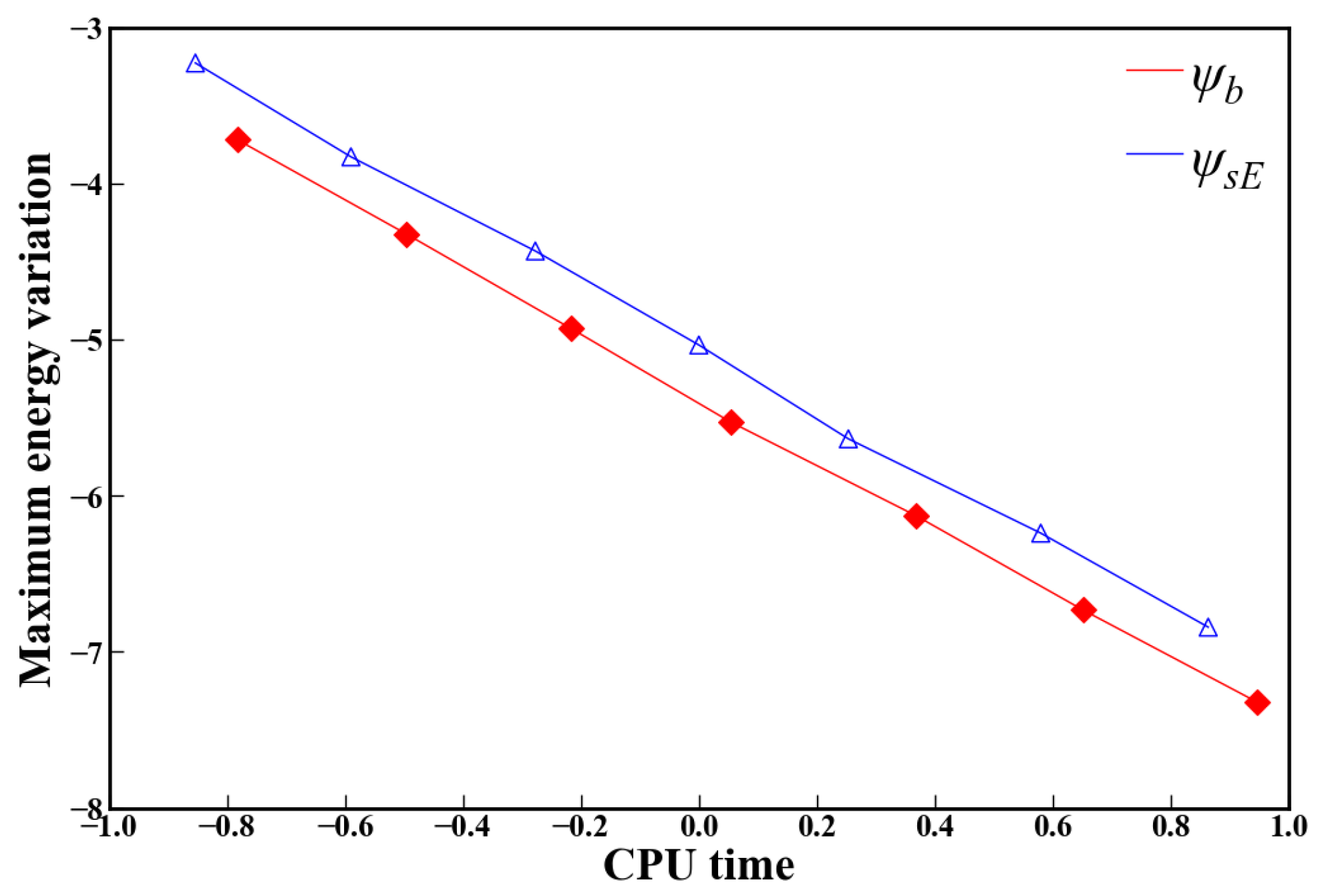
3. Energy Error Analysis

In this section, we analyze the energy deviation of the integrators ${\psi }_b$ over very long times. First, we consider ${\psi }_b$ and solve the modified differential equation whose solution $\mathbf{y}\left(t\right)$ formally satisfies $\mathbf{y}(n\Delta t)={\mathbf{x}}_n$. Thus, $\mathbf{y}\left(t\right)$ must satisfy Equation (5), i.e.,

$$\begin{array}{c}{\displaystyle \frac{\mathbf{y}(t+\Delta t)-2\mathbf{y}\left(t\right)+\mathbf{y}(t-\Delta t)}{\Delta t^2}}+\hfill \\ 2\mathsf{\Omega }\times {\displaystyle \frac{\mathbf{y}(t+\Delta t)-\mathbf{y}(t-\Delta t)}{2\Delta t}}=-\nabla \phi \left(\mathbf{y}\left(t\right)\right).\hfill \end{array}$$

(7)

We expand all terms into powers of $\Delta t$ at the time t then obtain the following modified differential equation

$$\begin{array}{c}(\ddot{\mathbf{y}}+\frac{\Delta t^2}{12}{\mathbf{y}}^{\left(4\right)}+\cdots )+\hfill \\ \mathsf{\Omega }\times (2\dot{\mathbf{y}}+\frac{\Delta t^2}{3}{\mathbf{y}}^{\left(3\right)}+\cdots )=-\nabla \phi \left(\mathbf{y}\right).\hfill \end{array}$$

(8)

Multiplying ${\dot{\mathbf{y}}}^{\top }$ in the two sides of the formula. Since ${\dot{\mathbf{y}}}^{\top }(\mathsf{\Omega }\times \dot{\mathbf{y}})=0$, we derive

$$\begin{array}{c}{\dot{\mathbf{y}}}^{\top }(\ddot{\mathbf{y}}+\frac{\Delta t^2}{12}{\mathbf{y}}^{\left(4\right)}+\cdots )+\hfill \\ {\dot{\mathbf{y}}}^{\top }\mathsf{\Omega }\times (\frac{\Delta t^2}{3}{\mathbf{y}}^{\left(3\right)}+\cdots )=-{\dot{\mathbf{y}}}^{\top }\nabla \phi \left(\mathbf{y}\right).\hfill \end{array}$$

(9)

The left-hand side can be written as the full differential and ${\dot{\mathbf{y}}}^{\top }\nabla \phi \left(\mathbf{y}\left(t\right)\right)=\frac{d}{dt}\phi \left(\mathbf{y}\left(t\right)\right)$, so the modified differential equation has a formal invariant, i.e.,

$$\begin{array}{cc}\hfill {\displaystyle \frac{d}{dt}}(& \frac{1}{2}{\dot{\mathbf{y}}}^{\top }\dot{\mathbf{y}}+\phi (\mathbf{y})+\frac{\Delta t^2}{12}({\dot{\mathbf{y}}}^{\top }{\mathbf{y}}^{\left(3\right)}-\frac{1}{2}{\ddot{\mathbf{y}}}^{\top }\ddot{\mathbf{y}}\hfill \\ \hfill & +4{\dot{\mathbf{y}}}^{\top }(\mathsf{\Omega }\times \ddot{\mathbf{y}}))+\cdots )=0.\hfill \end{array}$$

(10)

Thus, we obtain a new formal generalized energy $E_h(\mathbf{y},\dot{\mathbf{y}})=E(\mathbf{y},\dot{\mathbf{y}})+\Delta t^2{E}_2(\mathbf{y},\dot{\mathbf{y}})+\cdots$, which is an invariant. We only consider the numerical integrator $\left\{({\mathbf{x}}_n,{\dot{\mathbf{x}}}_n)\right\}$ in a compact set D. To estimate the energy error of the integrator ${\psi }_b$ over a long time, we truncate the $E_h$ in N leading terms, and integrate over the time interval $[0,n\Delta t]$,

$$\begin{array}{c}{E}_h^N({\mathbf{x}}_n,{\dot{\mathbf{x}}}_n)-E_h^N({\mathbf{x}}_0,{\dot{\mathbf{x}}}_0)=n\Delta t\mathcal{O}(\Delta t^N).\hfill \end{array}$$

(11)

The right-hand side in Formula (11) is a high order infinitesimal quantity, so

$$\begin{array}{c}|E({\mathbf{x}}_n,{\dot{\mathbf{x}}}_n)-E({\mathbf{x}}_0,{\dot{\mathbf{x}}}_0)|\le C_N\Delta t^2.\hfill \end{array}$$

(12)

where $C_N$ is directly dependent on the values of ${\dot{\mathbf{y}}}^{\top }{\mathbf{y}}^{\left(3\right)}-\frac{1}{2}{\ddot{\mathbf{y}}}^{\top }\ddot{\mathbf{y}}+4{\dot{\mathbf{y}}}^{\top }(\mathsf{\Omega }\times \ddot{\mathbf{y}})$ in the compact set D.

4. The Symplectic Property

In canonical Hamiltonian system, a map $\varphi :{\mathbf{z}}_n\mapsto {\mathbf{z}}_{n+1},\mathbf{z}\in {\mathbb{R}}^{2d}$ is called symplectic if its Jacobian matrix satisfies the symplectic condition,

$$\left({\displaystyle \frac{\partial \varphi }{\partial {\mathbf{z}}_n}}{)}^{\top }J\right({\displaystyle \frac{\partial \varphi }{\partial {\mathbf{z}}_n}})=J.$$

(13)

The equivalent form is that the map $\varphi$ preserves a standard symplectic structure $\frac{1}{2}d{\mathbf{z}}^{\top }\wedge Jd\mathbf{z}$, i.e., $d{\mathbf{z}}_{n+1}^{\top }\wedge Jd{\mathbf{z}}_{n+1}=d{\mathbf{z}}_n^{\top }\wedge Jd{\mathbf{z}}_n$.

In this subsection, we show that the numerical integrator ${\psi }_b$ is symplectic. We choose the discrete Lagrangian $L_h$ as

$$\begin{array}{c}{L}_h({\mathbf{x}}_n,{\mathbf{x}}_{n+1})=\frac{1}{2\Delta t}{({\mathbf{x}}_{n+1}-{\mathbf{x}}_n)}^2+\hfill \\ \frac{1}{2}\mathsf{\Omega }·({\mathbf{r}}_n+{\mathbf{r}}_{n+1})\times ({\mathbf{r}}_{n+1}-{\mathbf{r}}_n)-\Delta t\phi \left({\mathbf{x}}_n\right).\hfill \end{array}$$

(14)

The discrete form of ${\int }_{t_0}^{t_N}L(\mathbf{x}\left(t\right),\dot{\mathbf{x}}\left(t\right))dt$, i.e., the action $S_h$ is

$$S_h({\mathbf{x}}_0,\cdots ,{\mathbf{x}}_N)=\sum _{n=0}^{N-1}{L}_h({\mathbf{x}}_n,{\mathbf{x}}_{n+1}),$$

(15)

where $L_h$ is the discrete Lagrangian. According to the discrete Hamilton’s principle, the discrete Euler–Lagrange equation reads

$$\begin{array}{c}{D}_2{L}_h({\mathbf{x}}_{n-1},{\mathbf{x}}_n)+D_1{L}_h({\mathbf{x}}_n,{\mathbf{x}}_{n+1})=0,\hfill \end{array}$$

(16)

$$\begin{array}{c}{\mathbf{p}}_n=-D_1{L}_h({\mathbf{x}}_n,{\mathbf{x}}_{n+1}),\hfill \\ {\mathbf{p}}_{n+1}=D_2{L}_h({\mathbf{x}}_n,{\mathbf{x}}_{n+1}),\hfill \end{array}$$

(17)

where $D_i$ is the partial derivative with respect to the i-th argument. The corresponding formula of the formulation (17) is the formula (6). By eliminating ${\mathbf{p}}_n$, the evolution formulation of ${\mathbf{x}}_n$ can be obtained, which is ${\psi }_b$, as follows

$$\begin{array}{c}{\displaystyle \frac{{\mathbf{x}}_{n+1}-2{\mathbf{x}}_n+{\mathbf{x}}_{n-1}}{\Delta t}}+2\mathsf{\Omega }\times {\displaystyle \frac{{\mathbf{x}}_{n+1}-{\mathbf{x}}_{n-1}}{2}}=-\Delta t\nabla \phi \left({\mathbf{x}}_n\right).\hfill \end{array}$$

(18)

A straightforward calculation gives the equation of $d{\mathbf{p}}_{n+1}\wedge d{\mathbf{x}}_{n+1}=d{\mathbf{p}}_n\wedge d{\mathbf{x}}_n$ (refer to the Theorem 5.1 of Chapter 6 in Hairer [17]). It proves that the integrator ${\psi }_b$ is symplectic and defines a symplectic map $({\mathbf{p}}_n,{\mathbf{x}}_n)\mapsto ({\mathbf{p}}_{n+1},{\mathbf{x}}_{n+1})$.

It is also well-known that the symplectic integrator has the property of near-conservation of energy over a long time. The error expression (12) is estimated by taking into account the formal energy of the modified equation [18].

5. Numerical Experiments

In this section, we numerically present the behaviors of the integrator ${\psi }_b$ in two kinds of potential energy, an extensive Quadratic potential and restricted three-body Earth-Moon system. At the same time, we compare our results with those of the well-known symplectic Euler method ${\psi }_{sE}$ and the highly efficient Gauss Runge–Kutta method in the canonical form (4).

In the case of the canonical system, we make discrete the system (4) by the symplectic Euler method ${\psi }_{sE}$:

$$\left(\mathbf{a}\right):\left\{\begin{array}{cc}\hfill {\mathbf{x}}_{n+\frac{1}{2}}& ={\mathbf{x}}_n+\Delta t{H}_{\mathbf{p}}({\mathbf{x}}_n,{\mathbf{p}}_{n+\frac{1}{2}})\hfill \\ \hfill {\mathbf{p}}_{n+\frac{1}{2}}& ={\mathbf{p}}_n-\Delta t{H}_{\mathbf{x}}({\mathbf{x}}_n,{\mathbf{p}}_{n+\frac{1}{2}}),\hfill \end{array}\right.$$

(19)

and

$$\left(\mathbf{b}\right):\left\{\begin{array}{cc}\hfill {\mathbf{x}}_{n+1}& ={\mathbf{x}}_{n+\frac{1}{2}}+\Delta t{H}_{\mathbf{p}}({\mathbf{x}}_{n+1},{\mathbf{p}}_{n+\frac{1}{2}})\hfill \\ \hfill {\mathbf{p}}_{n+1}& ={\mathbf{p}}_{n+\frac{1}{2}}-\Delta t{H}_{\mathbf{x}}({\mathbf{x}}_{n+1},{\mathbf{p}}_{n+\frac{1}{2}}).\hfill \end{array}\right.$$

(20)

This numerical integrator ${\psi }_{sE}$ is a 2nd order explicitly symmetric symplectic numerical integrator for the canonical system (4). The explicit form of ${\psi }_{sE}$ reads

$$\left(\mathbf{a}\right):\left\{\begin{array}{cc}\hfill {\mathbf{x}}_{n+\frac{1}{2}}& =D{\mathbf{x}}_n+\Delta t{\mathbf{p}}_{n+\frac{1}{2}}\hfill \\ \hfill {\mathbf{p}}_{n+\frac{1}{2}}& =T({\mathbf{p}}_n-\Delta t\nabla U\left({\mathbf{x}}_n\right)),\hfill \end{array}\right.$$

(21)

and

$$\left(\mathbf{b}\right):\left\{\begin{array}{cc}\hfill {\mathbf{x}}_{n+1}& =T({\mathbf{x}}_{n+\frac{1}{2}}+\Delta t{\mathbf{p}}_{n+\frac{1}{2}})\hfill \\ \hfill {\mathbf{p}}_{n+1}& =D{\mathbf{p}}_{n+\frac{1}{2}}-\Delta t\nabla U\left({\mathbf{x}}_{n+1}\right).\hfill \end{array}\right.$$

(22)

In here, the matrices T and D are as follows

$$T=\left(\begin{array}{ccc}\frac{1}{1+{(\Delta tw)}^2}& \frac{\Delta t\omega }{1+{(\Delta tw)}^2}& 0\\ \frac{-\Delta t\omega }{1+{(\Delta tw)}^2}& \frac{1}{1+{(\Delta tw)}^2}& 0\\ 0& 0& 1\end{array}\right),D=\left(\begin{array}{ccc}1& \Delta t\omega & 0\\ -\Delta t\omega & 1& 0\\ 0& 0& 1\end{array}\right).$$

In addition, the 2nd order symmetric symplectic integrator ${\psi }_b$ is explicit, as follows

$$\begin{array}{cc}\hfill {\mathbf{x}}_{n+1}& =T(2{\mathbf{x}}_n-D{\mathbf{x}}_{n-1}-\Delta t^2\nabla \phi \left({\mathbf{x}}_n\right)).\hfill \end{array}$$

(23)

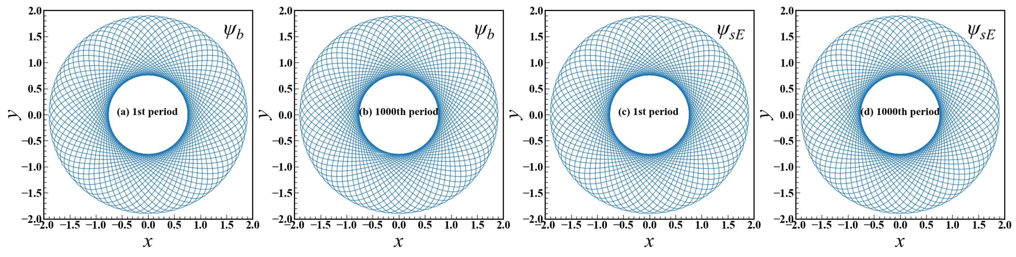
5.1. Quadratic Potential

We consider a homogeneous rotating top-hat density sphere with the quadratic potential of $U\left(\mathbf{x}\right)=4(x^2+y^2+z^2)$. We set the rotating speed $\omega =\pi /40$ and the period is 80. The initial position and velocity are $\mathbf{x}=(-1.9,0,0)$ and $\mathbf{v}=(0,-2.0,0)$, respectively.

We integrate the initial value problem in a time interval $[0,T]$ with $T=8\times {10}^4$ with different step-sizes $\Delta t=T/n$. We denote the maximum energy variation by

$${\mathrm{err}}_H(T/n)=\underset{k=1,\dots ,n}{\max }\left|\frac{H\left({\mathbf{z}}^k\right)-H\left({\mathbf{z}}^0\right)}{H\left({\mathbf{z}}^0\right)}\right|.$$

(24)

In Figure 2, we observe that the numerical integrators ${\psi }_b,{\psi }_{sE}$ both give the accurate orbit in the first rotation period and the 1000th rotation period. The work efficiency diagram of maximum energy variation along the trajectory versus the CPU time (in seconds) is displayed in Figure 3, both on the logarithmic scale. We observe that our integrator ${\psi }_b$ is more efficient than the integrator ${\psi }_{sE}$. In actually, with the same maximum energy variation, the efficiency of ${\psi }_b$ is increased by about $40\%$ versus ${\psi }_{sE}$.

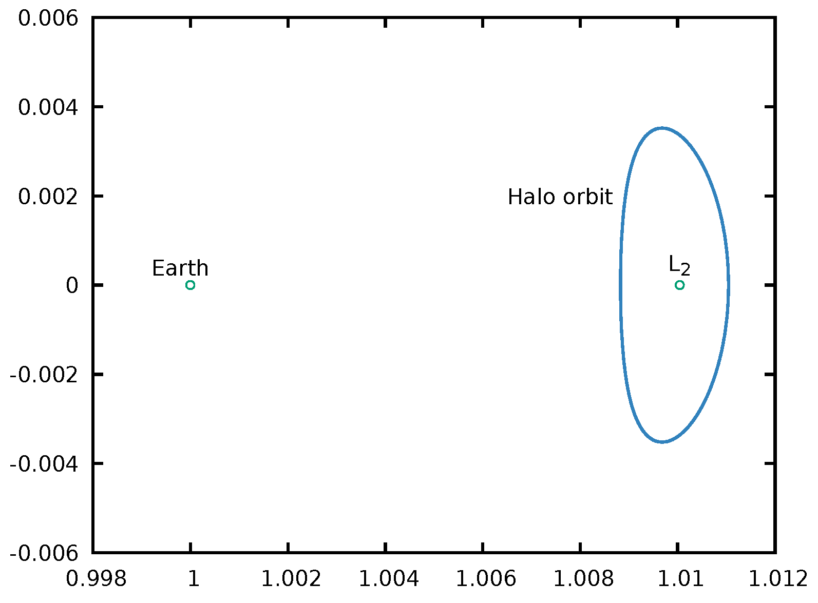
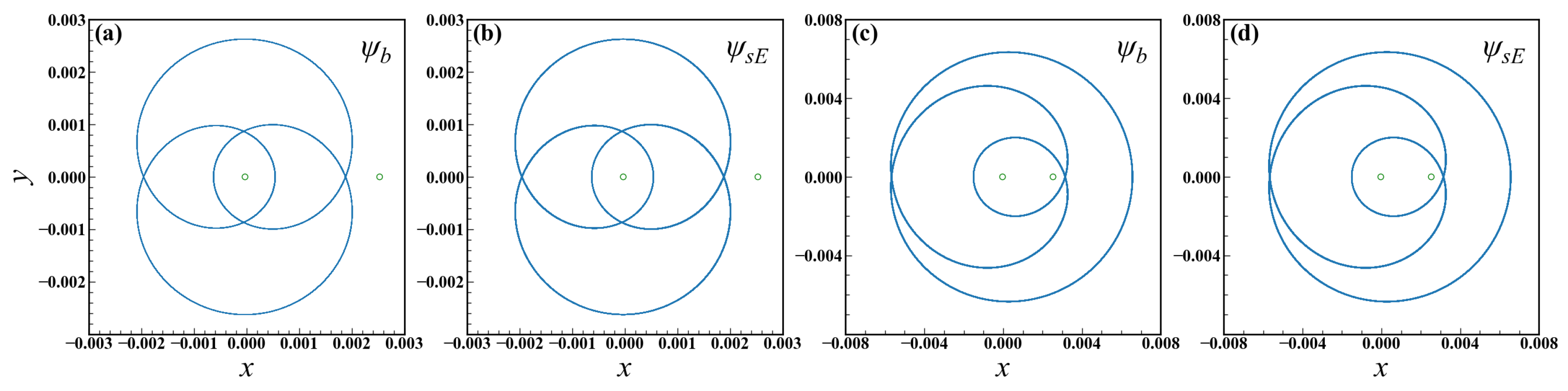
5.2. Earth-Moon System

In the design of a spacecraft’s orbit, the earth and moon’s disturbances should be taken into account, and the spacecraft can be seen as a mass point. In this case, the motions of the earth, moon, and satellite form a circular restricted three-body problem. The circular restricted three-body problem can be written in the form of (3) with potential

$$\begin{array}{cc}\hfill U\left(\mathbf{x}\right)=& -{\displaystyle \frac{G{M}_1}{\sqrt{{(x-x_1)}^2+{(y-y_1)}^2+z^2}}}\hfill \\ \hfill & -{\displaystyle \frac{G{M}_2}{\sqrt{{(x-x_2)}^2+{(y-y_2)}^2+z^2}}},\hfill \end{array}$$

(25)

which has been widely studied [15,16,19,20,21]. We expand into the component form of $(x,y,z)$, as follow

$$\begin{array}{cc}\hfill \frac{d^{2}x}{d{t}^2}-x{\omega }^2-2\omega \frac{dy}{dt}& =-\frac{G{M}_1(x-x_1)}{R_1^3}-\frac{G{M}_2(x-x_2)}{R_2^3},\hfill \\ \hfill \frac{d^{2}y}{d{t}^2}-y{\omega }^2+2\omega \frac{dx}{dt}& =-\frac{G{M}_1(y-y_1)}{R_1^3}-\frac{G{M}_2(y-y_2)}{R_2^3},\hfill \\ \hfill \frac{d^{2}z}{d{t}^2}& =-\frac{G{M}_{1}z}{R_1^3}-\frac{G{M}_{2}z}{R_2^3},\hfill \end{array}$$

where $R_1={({(x-x_1)}^2+{(y-y_1)}^2+z^2)}^{1/2},R_2={({(x-x_2)}^2+{(y-y_2)}^2+z^2)}^{1/2}$ and the coordinate origin is mass center of the system.

In this example of an Earth-Moon system, the unit of distance is an Astronomical Unit (1.4959787 × 10${}^{13}$ cm), the time unit is an earth day (86,400 s), and the mass unit is in kilograms. The corresponding normalized parameters $G{M}_1=$ 0.8997011603631609 × 10${}^{-9}$ (following the parameters in [22]), $G{M}_2=0.0123G{M}_1$, the distance of between earth and moon $R=$ 2.56267 × 10${}^{-3}$, $r_1=-M_{2}R/(M_1+M_2)=$−3.113784550034574 × 10${}^{-5}$, $r_2=M_{1}R/(M_1+M_2)=$ 2.531532154499654 × 10${}^{-3}$ and the rotation speed $\omega =\sqrt{G(M_1+M_2)/R^3}$. The earth position is $(x_1,y_1)=(r_1,0)$ and the moon position is $(x_2,y_2)=(r_2,0)$. We set two groups of initial conditions to check the behaviors of the numerical integrators ${\psi }_b$ and ${\psi }_{sE}$.

Orbit 1: we set initial position of the mass point at $\mathbf{x}=(-r_2/4,0,0)$, velocity $\dot{\mathbf{x}}=$ (0, 1.69561 × 10${}^{-3}$, 0). The orbit of the mass point is numerically integrated over a time interval $[0,4\times {10}^4]$.

Orbit 2: we set initial position of the mass point at $\mathbf{x}=(-3r_2/5,0,0)$, velocity $\dot{\mathbf{x}}=$ (0, 1.35057 × 10${}^{-3}$, 0). The orbit is integrated over a time interval $[0,{10}^5]$.

We integrate the initial value problem with different step-sizes $\Delta t=T/n$. Following the numerical experiment 1, the maximum energy variation is as follows

$${\mathrm{err}}_H(T/n)=\underset{k=1,\dots ,n}{\max }\left|\frac{H\left({\mathbf{z}}^k\right)-H\left({\mathbf{z}}^0\right)}{H\left({\mathbf{z}}^0\right)}\right|.$$

(26)

Figure 4 shows that for different initial values, the numerical integrators ${\psi }_b,{\psi }_{sE}$ both give the accurate orbit over a long time. Figure 5 shows that the work efficiency diagram of maximum energy variation along the trajectory versus the CPU time (in seconds) in double logarithmic scale with the initial values of orbit 1 and orbit 2. We conclude that our integrator ${\psi }_b$ is more efficient than the integrator ${\psi }_{sE}$.

5.3. High Order Composition Method

To show the strength of ${\psi }_b$, we construct the high order integrators ${\psi }_b^{10}$ and ${\psi }_{sE}^{10}$ by composition method, at the same time, we check the work efficiency of ${\psi }_b^{10}$ by comparing with ${\psi }_{sE}^{10}$ and the 10th order Gauss Runge–Kutta method ${\psi }_{grk}$.

At first, we present the one step integrator of ${\psi }_b$ [11] with the form of

$$\left\{\begin{array}{cc}\hfill {\mathbf{x}}_{n+\frac{1}{2}}& ={\mathbf{x}}_n+\frac{\Delta t}{2}{\mathbf{v}}_n\hfill \\ \hfill {\displaystyle \frac{{\mathbf{v}}_{n+1}-{\mathbf{v}}_n}{\Delta t}}& =-2\mathsf{\Omega }\times {\displaystyle \frac{{\mathbf{v}}_{n+1}+{\mathbf{v}}_n}{2}}-\nabla \phi \left({\mathbf{x}}_{n+\frac{1}{2}}\right)\hfill \\ \hfill {\mathbf{x}}_{n+1}& ={\mathbf{x}}_{n+\frac{1}{2}}+\frac{\Delta t}{2}{\mathbf{v}}_{n+1},\hfill \end{array}\right.$$

(27)

and

$$\left\{\begin{array}{cc}\hfill {\mathbf{x}}_{n+\frac{1}{2}}& ={\mathbf{x}}_n+\frac{\Delta t}{2}{\mathbf{v}}_n\hfill \\ \hfill {\mathbf{v}}_{n+1}& =T(D{\mathbf{v}}_n-\Delta t\nabla \phi \left({\mathbf{x}}_{n+\frac{1}{2}}\right))\hfill \\ \hfill {\mathbf{x}}_{n+1}& ={\mathbf{x}}_{n+\frac{1}{2}}+\frac{\Delta t}{2}{\mathbf{v}}_{n+1}.\hfill \end{array}\right.$$

(28)

It is well-known that one can obtain a higher order symmetric integrator by composition of the symmetric integrator. We derive the 10th order explicit, symmetric, symplectic integrator ${\psi }_b^{10}$ (and ${\psi }_{sE}^{10}$) by composition of the explicit, symmetric, symplectic integrator ${\psi }_b$ (and ${\psi }_{sE}$) using the best 35-stage method (Formula (17) in Sofroniou [23]). In addition, one can obtain an arbitrary high order integrator by the composition skills [17].

In our numerical implementation of the implicit Runge–Kutta method ${\psi }_{grk}$, we apply fixed point iteration with starting values computed by extrapolation from the previous step. Figure 6 shows that the work efficiency diagram of maximum energy variation along the trajectory versus the CPU times (in seconds) in double logarithmic scale, which are given by ${\psi }_b^{10}$, ${\psi }_{sE}^{10}$ and ${\psi }_{grk}$, the initial values are the orbit 1 and orbit 2 in the above numerical experiment 2. We conclude that our integrator ${\psi }_b^{10}$ is more efficient than ${\psi }_{sE}^{10}$ and ${\psi }_{grk}$.

6. Conclusions

In this paper, for the circular restricted three-body problem, we investigated the explicit symmetric numerical integrator ${\psi }_b$. In particular, the property of near-conservation of energy for long-term evolution and the symplectic property are derived for the integrator ${\psi }_b$. It is important that our 10th order explicit, symmetric, symplectic integrator ${\psi }_b^{10}$ is more efficient than the 10th order symplectic Euler method ${\psi }_{sE}^{10}$ and the 10th order implicit Gauss Runge–Kutta method ${\psi }_{grk}$ for the circular restricted three-body problem.

Two groups of numerical experiments, rotating quadratic potential and earth-moon system, are carried out to verify our theoretical analysis. In addition, the work efficiency comparison of the high order methods presented in Section 5.3 demonstrates the precision, high efficiency, and advantages of easy generation of high order methods of our method.

References

1. Feng, K. On difference schemes and symplectic geometry. In Proceedings of 1984 Beijing Symposium on Differential Geometry and Differential Equations; Feng, K., Ed.; Science Press: Beijing, China, 1985; pp. 42–58. [Google Scholar]
2. Feng, K. Difference Schemes for Hamiltonian Formalism and Symplectic Geometry. J. Comput. Math. 1986, 4, 279–289. [Google Scholar]
3. Forest, E.; Ruth, R.D. Fourth-order symplectic integration. Phys. D Nonlinear Phenom. 1990, 43, 105–117. [Google Scholar] [CrossRef]
4. Channell, P.J.; Scovel, C. Symplectic integration of Hamiltonian systems. Nonlinearity 1990, 3, 231–259. [Google Scholar] [CrossRef]
5. Candy, J.; Rozmus, W. A symplectic integration algorithm for separable Hamiltonian functions. J. Comput. Phys. 1991, 92, 230–256. [Google Scholar] [CrossRef]
6. Huang, L.Y.; Tian, Z.W.; Cai, Y.X. Compact Local Structure-Preserving Algorithms for the Nonlinear Schrödinger Equation with Wave Operator. Math. Probl. Eng. 2020, 2020, 4345278. [Google Scholar] [CrossRef]
7. Kong, L.H.; Chen, M.; Yin, X.l. A novel kind of efficient symplectic scheme for Klein–Gordon–Schrödinger equation. Appl. Numer. Math. 2019, 135, 481–496. [Google Scholar] [CrossRef]
8. Boris, J. Relativistic plasma simulation-optimization of a hybrid code. In Proceeding of Fourth Conference on Numerical Simulations of Plasmas; Naval Research Laboratory: Washington, DC, USA, 1970; pp. 3–67. [Google Scholar]
9. Qin, H.; Zhang, S.X.; Xiao, J.Y.; Liu, J.; Sun, Y.J.; Tang, W.M. Why is Boris algorithm so good? Phys. Plasmas 2013, 20, 084503. [Google Scholar] [CrossRef]
10. Ellison, C.L.; Burby, J.W.; Qin, H. Comment on “Symplectic integration of magnetic systems”: A proof that the Boris algorithm is not variational. J. Comput. Phys. 2015, 301, 489–493. [Google Scholar] [CrossRef]
11. He, Y.; Sun, Y.J.; Liu, J.; Qin, H. Volume-preserving algorithms for charged particle dynamics. J. Comput. Phys. 2015, 281, 135–147. [Google Scholar] [CrossRef]
12. Zhang, R.L.; Liu, J.; Qin, H.; Wang, Y.L.; He, Y.; Sun, Y.J. Volume-preserving algorithm for secular relativistic dynamics of charged particles. Phys. Plasmas 2015, 22, 044501. [Google Scholar] [CrossRef]
13. He, Y.; Sun, Y.J.; Liu, J.; Qin, H. Higher order volume-preserving schemes for charged particle dynamics. J. Comput. Phys. 2016, 305, 172–184. [Google Scholar] [CrossRef]
14. Hairer, E.; Lubich, C. Energy behaviour of the Boris method for charged-particle dynamics. BIT Numer. Math. 2018, 301, 969–979. [Google Scholar] [CrossRef]
15. Broucke, R.A. Periodic Orbits in the Restricted Three Body Problem with Earth-Moon Masses; Technical Report; Jet Propulsion Laboratory: Pasadena, CA, USA, 1968. [Google Scholar]
16. Murray, C.D.; Dermott, S.F. Solar System Dynamics; Cambridge University Press: Cambridge, UK, 1999. [Google Scholar]
17. Hairer, E.; Lubich, C.; Wanner, G. Geometric Numerical Integration: Structure-Preserving Algorithms for Ordinary Differential Equations, 2nd ed.; Springer: Berlin, Germany, 2006. [Google Scholar]
18. Tang, Y.F. Formal energy of a symplectic scheme for hamiltonian systems and its applications (I). Comput. Math. Appl. 1994, 27, 31–39. [Google Scholar]
19. Gao, F.B.; Zhang, W. A Study on Periodic Solutions for the Circular Restricted Three-body Problem. Astron. J. 2014, 148, 116. [Google Scholar] [CrossRef]
20. Perdomo, O. On the period of the periodic orbits of the restricted three body problem. Celest. Mech. Dyn. Astron. 2017, 129, 89–104. [Google Scholar] [CrossRef]
21. Abouelmagd, E.I.; Guirao, J.L.G.; Pal, A.K. Periodic solution of the nonlinear Sitnikov restricted three-body problem. New Astron. 2020, 75, 101319. [Google Scholar] [CrossRef]
22. Tu, X.B.; Murua, A.; Tang, Y.F. New high order symplectic integrators via generating functions with its application in many-body problem. BIT Numer. Math. 2020, 129, 509–535. [Google Scholar] [CrossRef]
23. Sofroniou, M.; Spaletta, G. Derivation of symmetric composition constants for symmetric integrators. Optim. Methods Softw. 2005, 20, 597–613. [Google Scholar] [CrossRef]
Figure 1. Halo orbit nearby the collinear libration point L 2 of Sun-Earth system. The James Webb Space Telescope is located in this Halo orbit.
Symmetry 14 01769 g001
Figure 2. The orbits are given by ψ b and ψ s E in the first rotation period (a,c) and the 1000th rotation period (b,d).
Symmetry 14 01769 g002
Figure 3. Maximum energy variation err H ( Δ t ) versus the CPU time in double logarithmic scale, which are given by ψ b and ψ s E over the time interval [ 0 , T ] .
Symmetry 14 01769 g003
Figure 4. Numerical orbits are given by ψ b , ψ s E with the initial values of orbit 1 (a,b) and orbit 2 (c,d), respectively.
Symmetry 14 01769 g004
Figure 5. Maximum energy variation err H ( Δ t ) versus the CPU time in double logarithmic scale, which are given by ψ b and ψ s E with the initial values of orbit 1 (left) and orbit 2 (right).
Symmetry 14 01769 g005
Figure 6. Maximum energy variation err H ( Δ t ) versus the CPU time in double logarithmic scale, which are given by ψ b 10 , ψ s E 10 and ψ g r k , the initial values are orbit 1 (left) and orbit 2 (right) in above numerical experiment 2.
Symmetry 14 01769 g006
Publisher’s Note: MDPI stays neutral with regard to jurisdictional claims in published maps and institutional affiliations.