Article

Long-Short Term Memory Technique for Monthly Rainfall Prediction in Thale Sap Songkhla River Basin, Thailand

1
Center of Excellence in Sustainable Disaster Management, School of Engineering and Technology, Walailak University, Nakhon Si Thammarat 80161, Thailand
2
Civil Engineering Department, College of Engineering, King Khalid University, Abha 61421, Saudi Arabia
3
Department of Physical Geography and Ecosystem Science, Lund University, Sölvegatan 12, SE-223 62 Lund, Sweden
4
Institute of Applied Technology, Thu Dau Mot University, Thu Dau Mot 75000, Vietnam
*
Authors to whom correspondence should be addressed.
Symmetry 2022, 14(8), 1599; https://doi.org/10.3390/sym14081599
Submission received: 21 June 2022 / Revised: 25 July 2022 / Accepted: 1 August 2022 / Published: 3 August 2022
(This article belongs to the Special Issue Time Series Forecasting in Physical Geography)

Abstract

:
Rainfall is a primary factor for agricultural production, especially in a rainfed agricultural region. Its accurate prediction is therefore vital for planning and managing farmers’ plantations. Rainfall plays an important role in the symmetry of the water cycle, and many hydrological models use rainfall as one of their components. This paper aimed to investigate the applicability of six machine learning (ML) techniques (i.e., M5 model tree: (M5), random forest: (RF), support vector regression with polynomial (SVR-poly) and RBF kernels (SVR- RBF), multilayer perceptron (MLP), and long-short-term memory (LSTM) in predicting for multiple-month ahead of monthly rainfall. The experiment was set up for two weather gauged stations located in the Thale Sap Songkhla basin. The model development was carried out by (1) selecting input variables, (2) tuning hyperparameters, (3) investigating the influence of climate variables on monthly rainfall prediction, and (4) predicting monthly rainfall with multi-step-ahead prediction. Four statistical indicators including correlation coefficient (r), mean absolute error (MAE), root mean square error (RMSE), and overall index (OI) were used to assess the model’s effectiveness. The results revealed that large-scale climate variables, particularly sea surface temperature, were significant influence variables for rainfall prediction in the tropical climate region. For projections of the Thale Sap Songkhla basin as a whole, the LSTM model provided the highest performance for both gauged stations. The developed predictive rainfall model for two rain gauged stations provided an acceptable performance: r (0.74), MAE (86.31 mm), RMSE (129.11 mm), and OI (0.70) for 1 month ahead, r (0.72), MAE (91.39 mm), RMSE (133.66 mm), and OI (0.68) for 2 months ahead, and r (0.70), MAE (94.17 mm), RMSE (137.22 mm), and OI (0.66) for 3 months ahead.

1. Introduction

Rainfall is one of the essential components in the hydrological cycle [1,2], playing a vital role in planning and managing water supply for symmetry with water demand from various activities, i.e., domestic household water consumption, industry, agriculture, etc. Rainfall variability is a natural factor affecting agriculture positively and negatively and creating risks and uncertainties in agricultural production. The Songkhla Sap basin is one of four main Southern River Basins of Thailand, mainly covering agricultural land of approximately 62.18 percent of the basin’s total area. The principal economic crops of this basin, i.e., rice, rubber, oil palm, fruit crops, etc., need water. Therefore, it is imperative to predict long-term rainfall for agricultural water management, including preventing and mitigating hazards posed by natural disasters such as floods and droughts. These issues create significant harm and danger to human life and property and agricultural products, leading to obstructing the area’s economic development.
However, rainfall prediction is complicated due to the nonlinear relationships between rainfall and climate variables. Wind, humidity, heat, earth rotation, and other significant factors impact rainfall [3]. In addition to the factors mentioned, climate change implications affect rainfall, especially in the coastal regions [4] and climate-sensitive areas such as the Southeast Asia region. This is because the region is located near the epicenter of variability caused by the interactions between the oceans, atmosphere, and land in the equatorial region between the Indian and Pacific Oceans [5]. It has been influenced by the southwest monsoon and northeast monsoon winds that blow through most of the year. In addition, the Indian Ocean Dipole (IOD) and El Niño-Southern Oscillation (ENSO) phenomena [6,7] results in rainfall variability in this region.
Previous studies have shown correlations between rainfall and climate variability in areas around the world. For example, Haq et al. [8] found that El-Nino 3.4 and IOD were strong enough to predict rainfall in Indonesia. Maass et al. [9] stated that the influence of ENSO is clearly dominant in the southern Pacific Coast of Jalisco, Mexico, with lower annual rainfall during hot periods called “La Nino” and higher annual rainfall during cold weather called the “Niña condition”. Islam and Imteaz [10] found that more than one climate index influenced rainfall in the southwest of Western Australia. A study by Chu et al. [11] suggested that the performance of predictive models with multiple climate factors was generally better than predictive models without climate factors, and several studies indicated that using climate indices could improve predicting efficiency, such as [4,12], etc. A number of studies have shown a correlation between rainfall estimates and ENSO/IOD in Thailand, such as [7,13,14,15,16]. The study’s findings all trend in the same direction. According to their research, ENSO is a factor impacting the variability in Thailand’s rainfall.
The rainfall prediction model can generally be classified into three main groups: conceptual models, physical models, and empirical models [17,18,19]. The conceptual model describes hydrological components. It requires large amounts of hydrological and meteorological data [20], and the conceptual models are usually lumped in nature and ignore the basin characteristics spatial variability and use the same parameters for the whole basin [21,22], with most model parameters having no direct physical meaning [23]. The physical model attempts to describe the physical processes which require variables or parameters about the initial state of the model and morphology of the basin [20]. The hydrological processes of water movement are represented by finite difference approaches such as partial differential equations [20,24]. Although such models produce satisfactory results, adjusting the parameters is time consuming [25]. The availability of data, the unpredictability of basins, and the complexity of such models may be unready and challenging to implement [26,27,28]. On the other hand, the empirical model is a data-driven model regardless of the basin’s hydrological component. As a result, they do not necessitate many parameters or data, resulting in a less complex and computationally efficient model [29].
In recent years, machine learning (ML) techniques capable of long-term analysis and big data have become increasingly popular in hydrology and water resources among researchers and engineers [30] because of their efficient tools in the estimation of rainfall and runoff [31]. It is a self-learning data-driven model. It is a branch of artificial intelligence that can find nonlinear relationships between input and output without the need for the knowledge of the fundamental physical processes of the basin [32,33]. For example, ML technologies were successfully applied in rainfall prediction [34], runoff simulation [35], pan evaporation prediction [36], solar radiation modeling [37], drought forecasting [38], and ground water level prediction [39]. Various ML models have been successfully applied for rainfall-runoff modeling [40], such as artificial neural network (ANN), multilayer perceptron (MLP), support vector regression (SVR), random forest (RF), M5 model tree (M5), and genetic programming (GP). Furthermore, recent technological advancements have led to a growing interest in deep learning (DL) methods—computer software that mimics the functions of the neural network in the human brain as a subset of ML. Through DL, one can automatically extract attributes from data that are strongly related to the dependent variable through hidden layers, whereas traditional ML methods must extract attributes from data that are strongly related to the dependent variable [18]. Modeling sequential data using recurring neural networks (RNNs) is one of the most active areas of DL research [41]. The long-short-term memory (LSTM) technique was created specifically for learning long-term dependencies by designing the functional part of the memory cell state in order to solve and overcome the vanishing gradient problem of traditional RNNs [18]. However, to our knowledge, not many studies have used DL in hydrology, especially for predicting rainfall. ML is a simple, low cost, and quick way of carrying out analysis and assessment, but it offers high efficiency and less complexity than commonly used models [33]. Consequently, many studies have attempted to use ML methods for predicting rainfall to reduce time and increase prediction efficiency.
For example, Hung, Babel, Weesakul, and Tripathi [40] used the ANN model to predict rainfall 1 to 6 h in advance for Bangkok. They found that the next 1 to 3 h were very satisfactory. While in the next 4 to 6 h, the prediction was not as accurate as it could be. Yu et al. [42] predicted rainfall in Taiwan and found that for 1 h ahead, both the RF and SVM models were satisfactory, but for 2 and 3 h ahead, the RF models underestimated the rainfall. Mekanik et al. [43] compared the ANN and MR (multiple regression) analysis, finding that ANN outperforms the MR analysis for predicting rainfall in Victoria, Australia. Ridwan et al. [44] developed and compared different ML methods for predicting rainfall in Tasik Kenyir, Terengganu. It was found that the different ML models could predict rainfall with an acceptable level of accuracy. The study results by Mislan et al. [45] showed that the ANN model could provide accurate rainfall predictions. While Zhang et al. [46] discovered that the SVR technique outperforms the MLP method for predicting yearly rainfall, both the SVR and MLP methods give accuracy at different intervals for non-monsoon rainfall. Choubin et al. [47] used large-scale climate as the model input to compare MLR (multiple linear regression), MLP, and ANFIS (adaptive neuro-fuzzy inference system) models for rainfall forecasting in the southwest of Iran. The results showed that large-scale climate had a significant effect on rainfall over the different lag times, with MLP outperforming other models. According to Aswin et al. [48], they used DL architecture models consisting of LSTM and ConvNet (convolutional neural network) to forecast global average monthly rainfall. The results showed that the model developed by DL provides accuracy and precision. Chen et al. [49] compared the ability of the LSTM and RF to forecast monthly rainfall at two Turkish meteorological stations using rainfall as the model’s input. The results showed that the LSTM model was more effective than the RF model. Kumar et al. [50] has used new deep learning models, namely, RNN and LSTM, for monthly rainfall forecasts in homogeneous rainfall regions of India. The outcomes demonstrate that deep learning networks can be successfully applied to hydrology time series analysis. The ML algorithm has been applied to other hydrology and water resource problems, for example, supporting runoff estimation models [51], water demand [52], simulation streamflow [53], predicting reservoir inflow [12], groundwater level prediction [54], and water quality evaluation [55], etc.
In a literature review, we found that all previous research applied LSTM for predicting rainfall with large data sets. This is because small data sets disrupt the ML training process. When training data sets become smaller, the model has fewer samples to learn from, increasing the risk of overfitting [56]. However, it is an inevitable problem, especially in developing countries with unavailable long recorded data. Most research used large data sets for predicting monthly rainfall of more than 40 years, such as [49,50,57,58]. One of the key issues with using ML to predict rainfall is its multi-step forecasting capability, which is vital for reliable hydrological forecasts to mitigate potential future risks [59,60]. Additionally, no previous publications have been found that LSTM was applied to predict multi-month-ahead of monthly rainfall with small data sets and studies that rely on large-scale climate data as variables for predicting rainfall using LSTM are still limited. To fill this research gap, especially in the tropical climate region, this research is the first attempt to investigate LSTM’s performance for multi-step-ahead prediction of monthly rainfall with small data sets and large-scale climate data.
The main aim of this paper is to (1) investigate the influence of climate variables on monthly rainfall, (2) investigate the applicability of LSTM with small data for monthly rainfall data set in tropical weather, and then compare traditional ML (i.e., M5, RF, SVR with polynomial and RBF kernels, and MLP), and (3) apply LSTM for multi-month-ahead rainfall prediction. This study chose two rain gauged stations in the Thale Sap Songkhla basin and nearby river basins. The rest of this article is organized as follows: Section 2 “Materials and Methods” includes the details of the study area and data analysis, and briefly describes the theories of machine learning algorithms, model development, and model performance evaluation. Section 3 presents the results and discussion of the findings. Section 4 provides the conclusions of this research.

2. Materials and Methods

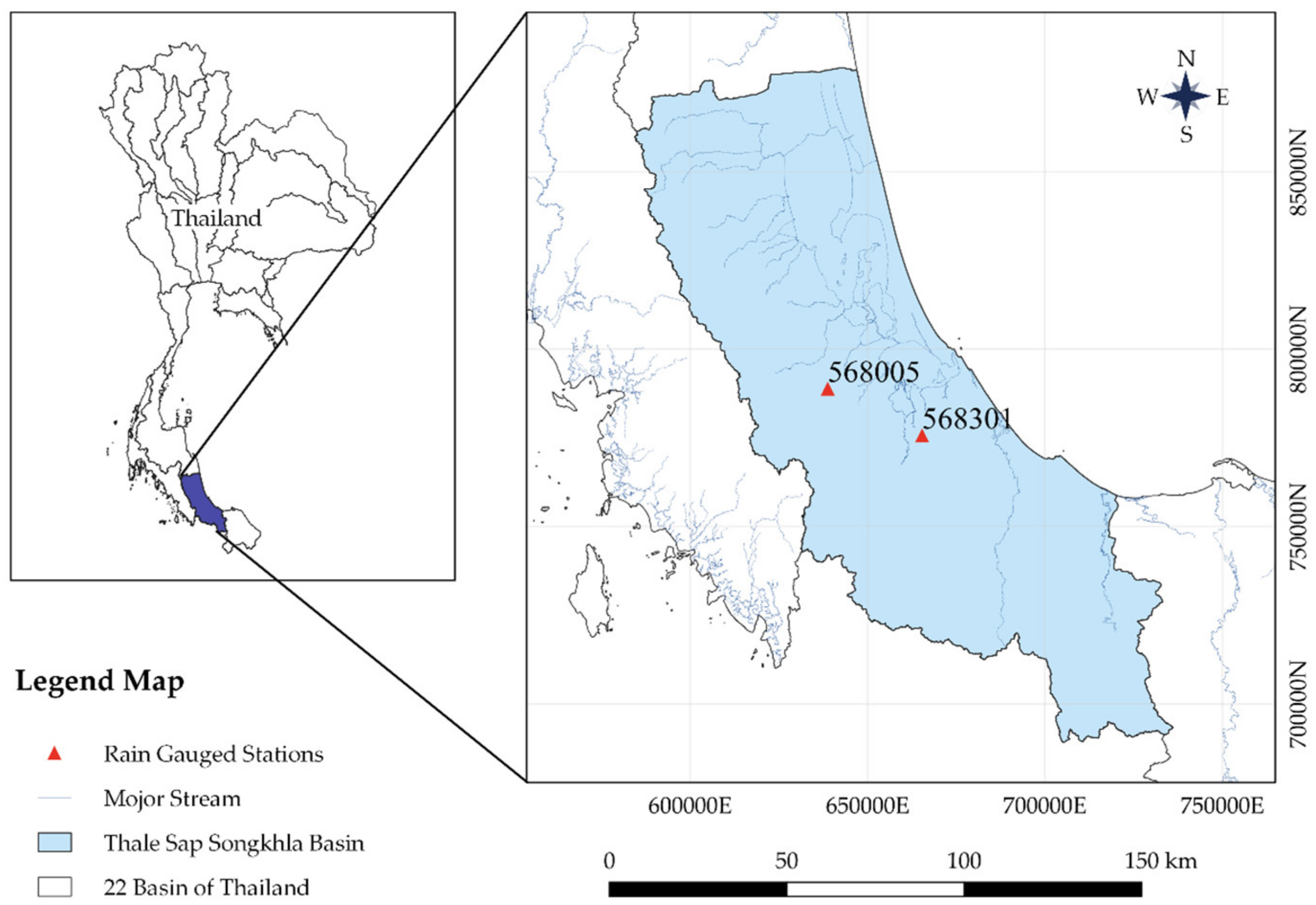
2.1. Study Area and Data Analysis

This study focused on the Thale Sap Songkhla River basin (TSSRB) in the southern region of Thailand (see Figure 1), situated at latitude 6°45′ and 8°00′ north and longitude 99°30′ and 100°45′ east. This river basin covers three provinces of Songkhla, Pattalung, and some parts of Nakhon Si Thammarat, with a total area of approximately 11,991.36 km2. The TSSRB is Thailand’s only watershed with a large lagoon-style lake system. The topography of the TSSRB consists of high mountainous areas in the west and south of the basin. The Bantad Mountain Range extends in the north and south directions in the west. On the south side is the San Kala Khiri Mountain Range, partially covered by fertile forest, thus being the source of watersheds that flow into Songkhla Lake. The northern and eastern parts of the TSSRB are coastal plains. The TSSRB is under the influence of the northeast monsoon and southeast monsoons. Therefore, there are two seasons of climate: summer and rainy seasons. The summer lasts from February to mid-July. The rainy season lasts from July to January, with the heaviest rainfall in November. The average annual rainfall in this area is approximately 2069.10 mm.
We collected meteorological data from the Thai Meteorological Department (TMD)’s weather stations located in the Thale Sap Songkhla basin: including monthly rainfall (two gauged stations), monthly air temperature, relative humidity, and wind speed (six gauged stations). In addition, we utilized three large-scale monthly data sets of oceanographic indices from the years 2004 to 2018, i.e., Southern Oscillation Index (SOI), Sea Surface Temperature (SST), and Indian Ocean Dipole Mode Index (DMI). SOI measures the differences in the atmospheric pressure above sea surface between Darwin and Tahiti in the Pacific Ocean. SST in the central Pacific Ocean notes as NINO1 + 2 (0–10S, 90W–80W), NINO3 (5S–5N, 150–90W), NINO3.4 (5S–5N, 170–120W), and NINO4 (5S–5N, 160–150W) from the National Oceanic and Atmospheric Administration (NOAA) website. DMI provides the difference in SST between the west and east coasts of the Indian Ocean from the Japan Agency for Marine-Earth Science and Technology (JMASTEC). In this study, the Thiessen method was deployed to determine basin areal rainfall using the QGIS program. It was introduced by Thiessen [61] for constructing polygons and calculating the weighted average. The summary statistical values of meteorological data and large-scale climate variables are presented in Table 1.

2.2. Machine Learning Models

2.2.1. M5 Model Tree

The M5 model tree is a method developed by Quinlan [62] based on the concept of the binary decision tree model and leaf regression function generation. The representation of knowledge in a tree structure makes it easy to understand, clear, and regression functions with few variables involved [63]. The M5 model tree is a model with non-linear functions. The model breaks a function into subsets and builds a linear regression model to determine the relationship of the data set in each subset.
The total data set (T) is divided into several subsets ( T i ) by splitting the criterion as shown in Figure 2, which depends on the standard deviation of the class obtained in T to measure the error at that instance and calculate the standard deviation reduction (SDR) as Equation (1) in each attribute at a sub-instance to select the best attribute, which gives the most SDR value. This process is repeated until the data set is divided into several subsets, until the attribute’s class value is very small or when the standard deviation ( T i ) is less than the standard deviation (T) of the original instance set.
SDR = sd T T i T sd T i

2.2.2. Random Forest

Random forest (RF) is an ensemble learning machine introduced by Breiman [64] that produces excellent results even without hyperparameter tuning. This model is not affected by overfitting. It can capture nonlinearity and has few model parameters. The RF is one of the most used models because its simplicity and diversity can be applied to both classification and regression problems. RF is used to create a decision tree with a large number of trees, where each tree is generated from training data at bootstrap and randomly selects a subset of data attributes, with each node receiving a unique data set. The model determines the output by using the average of the output from the tree clusters through the decision tree to predict the outcome. Increasing the number of trees increases the accuracy of the results. Figure 3 shows architecture of a random forest model.

2.2.3. Support Vector Regression

Support vector regression (SVR) is a supervised learning model that uses the support vector machine (SVM) methodology. It is one of the powerful models that can be used in the problem of classification when data cannot be linearly separated. Support vector regression relies on the same basic principles as the support vector machine but applies it to regression-type problems. The normal principle of regression is based on a single line, but this method draws the best boundary line to the regression, meaning it covers the most observations using the loss function “Epsilon Intensive Loss Function” (see Figure 4), which is the acceptable error value in absolute terms. The observation point outside the ε-tube region is the model’s error value, while the observation points inside the ε-tube region are zero error. The purpose of SVR is to try to provide all the observation data inside the boundaries (minimal error). The SVR model is adapted from the SVM model, so the SVR regression equation is similar to SVM’s hyperplane equation, with the goal of finding a linear relationship between the input vector and the output variable. The SVR regression function by Vapnik [66] can be described using Equations (2) and (3).
f x = wx + b = i = 1 l α i α i K x i x + b
subject   to i = 1 l α i α i = 0 0 α i C , 0 α i C
where w is a weight vector, x is the nonlinear transfer function, b is the bias, α i , α i is a Lagrange multiplier, and K x i x is a linear kernel function used to handle high-dimensional feature space. Since the data set is actually non-linear, having a kernel function can change data with lower dimensions to higher dimensions to allow for linear model division [67], the proper selection of kernel functions can produce more results or accuracy. Popular kernel functions such as:
  • Linear kernel
    K x i , x = x i , x
  • Polynomial kernel
    K x i , x = 1 + x i · x d
  • RBF kernel
    K x i , x = exp γ x i x 2
Figure 4. Nonlinear and linear SVR with Vapnik ε-insensitive loss function (Source: Adapted from Yu et al. [68]).
Symmetry 14 01599 g004

2.2.4. Multilayer Perceptron

The original idea of the artificial neuron network (ANN) was developed by McCulloch and Pitts [69], which proposed a concept based on the behavior of the human brain and neuronal relationships, requiring computers to be capable of learning to know, analyze, and make decisions similar to human beings. A multilayer perceptron (MLP) neural network is a form of a multilayer-structured feed-forward neural network trained using a backpropagation learning algorithm. Figure 5 presents a multi-layer perceptron with two hidden layers. The main strength of MLP is its non-linearity. Usually, MLP is organized into a set of interconnected layers of neuron cells consisting of an input layer, hidden layer, and output layer. The input layer receives the data and the hidden layer processes them, and finally, the output layer displays the resulting model output. The structure of the MLP neural network is a simple neural network structure, thus being a simple and complex structure. The mathematical equation can be expressed as follows.
y = φ i = 1 n w i x i + b
where w is the vector of weights, x is the vector of inputs, b is the bias, φ is the non-linear activation function, and y is the output. There are many activation functions to choose from. The one of popular activation function in the past was the logistic activation function (Sigmoid: σ), which is a function that takes whatever data are entered and changes them to a value between 0 and 1. The equation is as follows:
f x = 1 1 + e x

2.2.5. Long-Short Term Memory

Long-short-term memory (LSTM) was proposed by Hochreiter and Schmidhuber [71] as a type of network developed from RNNs. However, RNN can only view historical data for a short time. Therefore, it is not powerful enough to learn patterns from long-term dependencies. This will cause issues with backpropagation because it will need to go back many steps and nodes. As a result, the vanishing gradient problem occurs. Therefore, the LSTM technique was explicitly created for learning long-term dependencies by designing the functional part of the memory cell state to solve and overcome the weaknesses of traditional RNNs. In the LSTM memory cells, a “gate” unit controls the information that will be entered into each node, consisting of the forget gate, input gate, and output gate. The forget gate is a gate that has to determine whether the information that comes in the cell state should be stored or should be left. The input gate is a gate that has to receive new information and then record or write data in each node, which will decide whether to update the value or not update it with any value. Then, send that value to the output gate to decide whether to show that information or return it. Therefore, LSTM can learn from the data that are sequential and can collect or delete data if the data are not necessary. Figure 6 depicts the structure of the LSTM, and the formulas are as follows:
  • Forget gate
    f t = σ W f · x t , h t 1 + b f
  • Input gate
    i t = σ W i · X t , h t 1 + b i
  • Cell state candidate
    C ¯ t = tan h W c · x t , h t 1 + b c
  • Cell state
    C t = f t     C t 1 + i t     C ¯ t
  • Output gate
    o t = W o · X t , h t 1 + b o
  • Hidden state
h t = o t tan h C t
where W and b are the weight matrices and bias, x t is the input to the memory cell, h t 1 is the hidden state at time t − 1, C t 1 and C t are the cell states at time t − 1 and t, σ and tanh are the activation functions of the logistic sigmoid function and σ and tanh are the hyperbolic functions (tanh) with values between [0, 1] and [−1, 1], respectively. The format of the internal operating system of the LSTM may be modified as appropriate for each task.
Figure 6. The structure of the long-short-term memory (LSTM) neural network (Source: Adapted from Van Houdt et al. [72]).
Symmetry 14 01599 g006
As previously mentioned, there are many activation functions to choose from; however, the most used activation functions in ANN and deep learning are sigmoid, tanh, and Relu. Sigmoid is an S-curve function. The output of the sigmoid function is between 0 and 1. It is suitable for use in applications that require a probability output. However, it suffers from vanishing gradient problems [73] where neurons tend to stop learning to some extent. Then, Tanh activation function was proposed. The Tanh function, or hyperbolic tangent activation function, is a function that solves many of the disadvantages of sigmoid but has the same S shape. The output value of tanh is between −1 and 1. For this reason, the hyperbolic tangent curve is steeper than the sigmoid curve. Hence, the derivatives are durable, which, when compared to sigmoids, lessens the gradient lost [74]. However, the missing gradient issue still occurs in the tanh function when moving to a deeper network. Relu, short for rectified linear unit, is a linear function that is not S-shaped, such as the two previous functions. The Relu function expands the range from 0 to ∞, meaning that if the input is greater than zero, the output is positive. Additionally, if the input is zero or negative, then the output is zero, which is somewhat higher than the sigmoid and tanh functions. ReLU is a simpler function than all previous activation functions. This is because if the input is positive, the slope is always one. This reduces the vanishing gradient problem [73], allowing us to train the model faster. However, it cannot update the negative weight, but the advantage is that that gradient does not disappear, which overcomes everything and allows the drawbacks to be overlooked.

2.3. Model Development

In this study, six ML methods were selected and compared, M5, RF, SVR-poly, SVR-rbf, MLP, and LSTM, as alternative techniques for predicting monthly rainfall at two weather stations located in the Thale Sap Songkhla. Weka (Waikato Environment for Knowledge Analysis), free and open-source software, and ANNdotNET, a NET-based solution consisting of a set of tools for running deep learning models, were utilized. The total data set of 165 data sets, or 165 months, is the data obtained after pre-processing, which was partitioned into a training set and testing set. A training set is a data set used to teach a machine learning model to learn the appropriate parameters, while a testing set is used to evaluate the model’s performance. The study used a ratio of 70:30, i.e., 70% (115 data sets) for the training set and 30% (50 data sets) for the testing set. Additionally, the rainfall predicting procedures are summarized as follows:
Step 1: Input selection. Selecting input data is one of the most important issues in predictive model development and significantly affects model performance [75]. The data obtained may contain many attributes or variables, which may or may not be related to the dependent variable. Therefore, for the most accurate analysis of dependent variables, only attributes related to dependent variables should be selected as input models. In many studies, mostly for simplicity, rainfall was the only input [3,45,76]. This study used climate variable data for the rainfall prediction based on Pearson’s correlation
Step 2: Tuning hyperparameters. Another improvement in model performance is to adjust parameters, also known as hyperparameters. This is a parameter adjustment to select the most suitable set of parameters [77] using a trial-and-error process until the best prediction score is obtained. Consistent with the study by Ridwan, Sapitang, Aziz, Kushiar, Ahmed, and El-Shafie [44], they found that without tuning, the model (boosted decision tree regression) performed poorly, but when tuned, the accuracy of the model was noticeably increased
Step 3: Influence of climate and meteorological variables on monthly rainfall. Three scenarios of input patterns were examined to study the influence of climate and meteorological variables on one-month-ahead monthly rainfall predictions. The most straightforward and most efficient model would propose for the model’s applicability.
  • Scenario1: ML models with large-scale climate and meteorological variables as inputs.
  • Scenario2: ML models with only meteorological variables as inputs.
  • Scenario3: ML models with only rainfall variables as an input.
Step 4: Multi-month-ahead rainfall prediction. We selected the best scenario of input pattern from these three scenarios for each gauged station to predict multi-month-ahead rainfall. Additionally, the projected rainfall of the current time step was used as input data for the next step, as shown in Figure 7.

2.4. Model Performance Evaluation

In this study, statistical indicators were used as criteria for assessing the effectiveness of the model, namely, correlation coefficient (r), mean absolute error (MAE), root mean square error (RMSE), and overall index (OI).
The r measures the strength and direction of the linear relationship between two variables. Its values range between −1 and 1. If r is close to 1, the two variables are highly correlated and have the same direction [79].
r = i = 1 n R obs   R ¯ obs R sim   R ¯ sim i = 1 n ( R obs   R ¯ obs ) 2 · i = 1 n ( R sim   R ¯ sim ) 2
MAE and RMSE are measurements of the average magnitude of the error. It shows up in the form of an error between the simulated values produced by the model and the observed values. MAE and RMSE range from 0 to . Lower values are better because MAE and RMSE are negatively oriented scores.
MAE = i = 1 n R obs R sim n
RMSE = i = 1 n R obs R sim 2 n
The OI indicator is a criterion that indicates the overall performance of a model, with values ranging between −∞ and 1 [80] r, MAE, RMSE, and OI are defined by the following equations.
OI = 1 2 2 RMSE R obs , max R obs , min i = 1 n R obs R sim 2 i = 1 n R obs   R ¯ obs 2
where R obs denotes the observed rainfall, R cal denotes the calculated rainfall, R ¯ obs denotes the average observed rainfall, R ¯ cal denotes the average calculated rainfall, R obs , max denotes the maximum observed rainfall, R obs , min denotes the minimum observed rainfall, and n denotes the number of rainfall data.

3. Results and Discussion

3.1. Input Selection

A set of inputs at lags of 1, 2, 3, …, 12 months were used to predict the rainfall. Using analysis, attributes with a correlation coefficient (r) value higher than 0.25 were selected as the model’s nominated input variables. Figure 8a–c show the two stations’ correlation between rainfall and the climate variables of lead time at t + 1, t + 2, and t + 3 months, respectively. We found that the delay was appropriate for correlation analysis, with each climate variable showing different maximum relevant results.
While the deep learning model’s selection of features and classifiers is automated, the neural network learns which feature to choose. In contrast, traditional machine learning models require scientists or users to extract data and create features to make learning algorithms work by reducing the complexity of the data and making patterns more visible. This is an advantage of deep learning over the traditional machine learning models.
For large-scale climate variables, correlations between rainfall and SOI were positively and negatively weak (r = −0.06 to 0.17). Rainfall and SOI have a direct relationship since a negative SOI value results in higher temperatures, lower rainfall or drought conditions (El Niño) and periods of high rainfall (La Niña), and positive SOI values result in low temperatures and increased rainfall [81] as seen from Figure 9a. In addition, the correlation between rainfall and DMI was the weakest (r = −0.08 to 0.11). There were no stations with a DMI greater than 0.25, implying that DMI was not chosen as an input variable for all stations. Similarly, we found that the climate indices having the greatest influence on two weather gauged stations in the Songkhla Lake basin were SST: NINO1 + 2 (r = −0.5 to 0.5), NINO3 (r = −0.43 to 0.43), NINO3.4 (r = −0.29 to 0.26), and NINO4 (r = −0.28 to 0.10). The relationship between rainfall and DMI/SST is inverse, where positive DMI and SST result in reduced rainfall or drought (El Niño). In contrast, negative SST results in high rainfall (La Niña) [14], demonstrated in Figure 9b,c. Our study is consistent with a study by Sein et al. Sein et al. [82] that found that SOI had a greater influence on rainfall in neighboring Myanmar than IOD (DMI).
Meteorological variables (i.e., air temperature: T; relative humidity: RH; wind speed: WS; and rainfall: R) were significantly related to rainfall. T and WS (r = −0.43 to 0.47) were inversely related to the present rainfall, as shown in Figure 9d,f, while RH (r = −0.38 to 0.44) and R (r = −0.22 to 0.50) had a direct relationship with the present rainfall. As shown in Figure 9e, the relationship between RH and R shows that as the relative humidity increases, precipitation also increases. RH is the main factor in cloud formation resulting in rainfall. Rainfall chances are lower as the wind speed increases. The northeast monsoon blowing between October and February influences the rain in the Gulf of Thailand. However, during January and February, there is considerably less rainfall. This clearly shows the variability in rainfall. However, such factors depend on the geographical features of each area as well. In addition, the increase in air temperature results in a decrease in the amount of rainfall. The high air temperature favors very hot and dry conditions.

3.2. Tuning Hyperparameters for Machine Learning Methods

This study used the Weka Experiment Environment for trial and error. The lowest root relative squared error value (RRSE) was used to select the best parameter. However, for ANNdotNet (LSTM), we used a trial-and-error method and observed the best parameters from an efficiency standpoint since there is no tool for tuning parameters. Table 2 shows the optimal model parameters, which can be explained as follows.

3.2.1. M5 Model Tree

In the M5 model, three parameters were investigated: batchSize, minNumInstances, and numDecimalPLaces. The batchSize option specifies the recommended number of instances to handle if the batch prediction is used. It is possible to offer more or fewer instances. However, this allows the implementation of a preferred batch size. The minimum number of instances to allow at a leaf node is minNumInstances. Bae et al. [83] explained that minNumInstances is implemented to prevent overfitting in a regression function. numDecimalPLaces is the number of decimal places to be used for the output of numbers in the model. Overall, batchSize of 100, minNumInstances ranging from 4 to 30 and numDecimalPLaces of 4 are appropriate hyperparameters for an M5 model tree with a testing data set. All two gauged stations gave RRSE values in the range of 85.15–99.46. We found that minNumInstances is a sensitive parameter. Due to the increase in the value of minNumInstances, the model is overfitting, and decreasing the minNumInstances value allows the model to reduce excessive complexity, which corresponds to Bae, Han, Lee, Yang, Kim, Lim, Neff, and Jang’s [83] statement that the parameter minNumInstances prevents overfitting in the regression function, while batchSize and numDecimalPLaces were not sensitive.

3.2.2. Random Forrest

RF have several default parameters in WEKA software; however, three parameters (i.e., bathSize, numIteration, and numExecutionSlots) were selected in this study. The bathSize is as described in section M5. The numIteration is the number of trees in the random forest, while numExecutionSlots is the number of execution slots (threads) to construct the ensemble. Findings revealed that a batchSize of 100, numIteration ranging from 100 to 100 and numExecutionSlots of 1 are appropriate hyperparameters for an RF with a testing data set. Both stations gave RRSE values in the range of 78.93–96.02. The numIteration was a sensitive parameter. Having a number of trees means that it takes a long time to run the model. Their larger numbers improve model performance until a certain point, after which the number of trees no longer affects model performance. The batchSize and numExecutionSlots were not sensitive.

3.2.3. Support Vector Regression

The performance of the SVR model is dependent on the kernel function and model parameters selected. This study examines two kernel functions: a polynomial kernel function and a radial basis function (RBF). The SVR’s parameterization involves the adjustment of the regularization parameter, namely, complexity parameter (C) and epsilon parameter (ε). It also concerns parameters in two kernel functions: i.e., the exponent parameter (n) of the polynomial kernel function and the gamma parameter (γ) of the radial basis function. The C defines the extent to which the data set or margin can be placed and the ε parameter of the epsilon insensitive loss function. The value of ε can affect the number of supporting vectors used to construct the regression function. A larger ε value results in fewer support vectors, whereas a smaller ε value makes the model more flexible [84].
We found that the optimal hyperparameters for SVR with polynomial kernel functions (SVR-poly), C ranging from 0.1 to 50, ε ranging from 0.0001 to 0.1, and n of 1.0 were appropriate. Moreover, it gave RRSE values ranging from 80.57 to 94.16. The SVR with the radial kernel function (SVR-rbf) provided the parameter C in the range of 0.1 to 100 and ε in the range of 0.0001 to 0.1, and γ; ranging from 0.01 to 0.5. It gave RRSE values ranging from 74.72 to 94.70. Additionally, we find that the γ parameter is very sensitive. It can be seen that in both cases there is a small value of parameter C, indicating that it is possible to find outliers in the general decision boundary. In contrast, large C values limit the possibility of outliers and determine more precise decision boundaries. Maximizing the C value for the decision region shows good results [83]. If C is large, the model may be overfitting, whereas if C is small, the model may be underfitting. However, it depends on the data set.

3.2.4. Multilayer Perceptron

For MLP, we focused on parameter tuning related to network structure (hidden layer) and hyperparameters related to the training algorithm (i.e., momentum, learning rate, and training time). The hidden layer defines the hidden layers of the neural network. To adjust the hidden layer, we specify a wildcard value consisting of “a” ((attributes + classes)/2), “I” (attributes), “o” (classes), “t” (attributes + classes)). As previously stated, MLP is linked to weight and bias, so the learning rate is applied to weight and bias updates, momentum is applied to weight updates, and the training time is the number of epochs to train through. We found that the optimal number of hidden layers was two, and in terms of the learning rate, momentum, and training time, the ranges were from 0.1 to 0.5, 0.1 to 0.5, and 100 to 1000, respectively, with RRSE values ranging from 84.87 to 115.76. The learning rate and training time are pretty sensitive to our data set. When both are large, the model is overfitting.

3.2.5. Long Short-Term Memory

For LSTM, we have adjusted two parameters consisting of (1) visual network designer, which allows the visual creation of different types of deep network architecture (i.e., normalization layer, LSTM layer, dense layer, output layer), and (2) the learning and training parameters (i.e., learning rate, momentum, number of epochs, and progress frequency). The normalization layer takes the numerical features and normalizes their values at the beginning of the network. The dense layer is a classic neural network layer with an activation function. The LSTM is a special version of the recurrent network layer with an option for peephole and self-stabilization. We found that the optimal number of the normalization layer was one layer, the LSTM layer was one layer, the dense layer was two layers, and the output layer was one layer. The ideal values for the LSTM were layer and cell dimensions in the range of 70 and 80 and dense layer dimensions ranging from 10 to 50. The output was only one, and the layer dimension was 1. The learning rate ranging from 0.1 to 0.9, momentum 1, the number of epochs of 1000, and progress frequency of 10 were optimal hyperparameters for this model. The findings revealed that the suitable activation functions with good performance for the LSTM layer, dense layer 1, dense layer 2, and output layer were tanh, tanh, Relu, and Relu, respectively.

3.3. Influence of Climate Variables on Monthly Rainfall and Model Performance Comparison

Figure 10 shows a bar graph comparing three scenarios with different input variables. It shows the influence of climate variables on rainfall prediction performance at 1 month lead time. OI is the performance indicator used to choose the best scenarios. For the training period, we discovered that most methods for the 568005 and 568301 stations gave higher OI values in scenario 1 than in scenarios 2 and 3, except for the MLP method on the 568005 station and the RF and SVR-poly on the 568301 gauged station. When considering the average, scenario 1 had a higher OI average than scenario 2, indicating better performance. In comparison, scenario 3 has a lower average than scenarios 1 and 2. For the testing period, we discovered that the OI value of the situation where scenario 1 is lower than other at the 568005 station and one method at the 568301 gauged station. However, when considering the average value, scenario 1 still has a slightly higher OI average than scenario 2. Scenario 3 had a lower average than scenarios 1 and 2. It indicated that large-scale climate variables were clearly a factor influencing monthly rainfall predictions. However, rainfall alone is not enough to predict rainfall in this basin, resulting in the complex model being more suitable for our study. In conclusion, scenario 1 was the most suitable model input variable.
Table 3 shows a comparison of the model performance criteria matrix, including r, MAE, RMSE, and OI, for two rainfall stations. As mentioned previously, the ML model type, giving the highest performance for 1-month lead time, was selected to develop a model for predicting monthly rainfall at 2- and 3-month lead times. The model training period performed better than the testing period, specifically the RF model. This evidently might show the overfitted model. The LSTM model was the most popular among both stations when considering the testing period. The efficiency values r, MAE, RMSE, and OI for the 568005 gauged station were 0.74, 88.63 mm, 128.11 mm, and 0.70, respectively. Additionally, those values for the 568301 gauged station were 0.75, 83.99 mm, 130.09 mm, and 0.70, respectively. While MLP provides the lowest performance for both stations, the methods of SVR-rbf, SVR-poly, RF, and M5 for the 568005 gauged station and SVR-poly, SVR-rbf, M5, RF for the 568301 gauged station provided an inferior performance compared to LSTM, respectively.

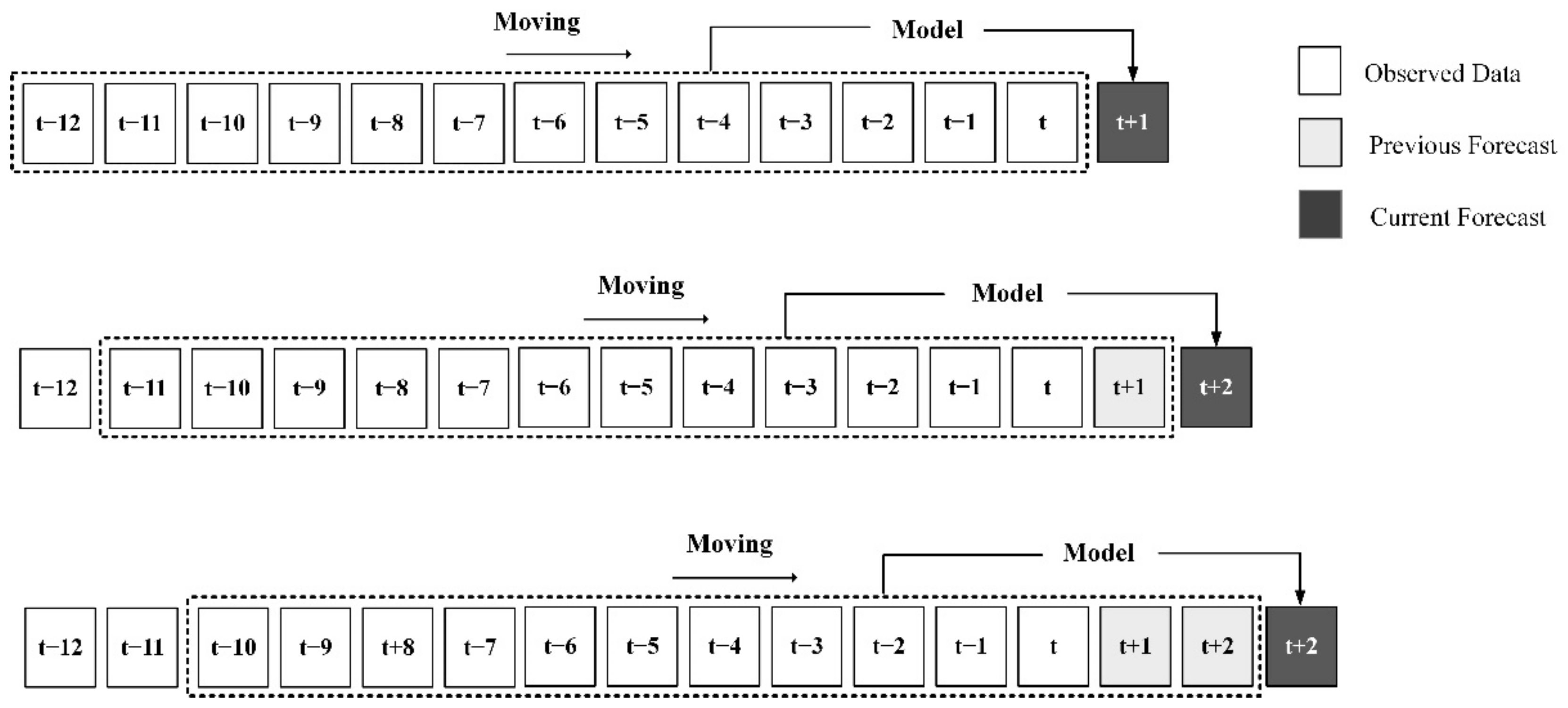
3.4. Multi-Month-Ahead Rainfall Predicting

The LSTM model was identified as the best among the six ML models, according to the preliminary testing. Therefore, it was further applied in the multi-month rainfall prediction (lead time = 1, 2, and 3 months) at two weather gauge stations. Table 4 shows the performance criteria matrix of the different multi-month models: r, MAE, RMSE, and OI. The LSTM model provided a little difference in the rainfall predictions for the lead times of 1, 2, and 3 months. Evidently, as the prediction time increases, the efficiency gradually decreases.
At a lead time of 1 month, when considering the testing period, r, MAE, RMSE, and OI for the 568005 gauged station were 0.74, 88.63, 128.11, and 0.70, respectively, and for the 568301 gauged station they were 0.75, 83.99, 130.09, and 0.70, respectively. This reflects satisfactory results. Predicting performance at a lead time of 2 months was a little less satisfactory with r, MAE, RMSE, and OI values of 0.73, 89.03, 134.23, and 0.68 for the 568005 gauged station, and 0.72, 93.75, 133.09, and 0.69 for the 568301 gauged station, respectively. Finally, for a lead time of 3 months, efficiency values were a little lower than those at the lead times of 1 and 2 months, with r, MAE, RMSE, and OI being 0.71, 96.48, 134.74, and 0.67 for the 568005 gauged station and 0.69, 91.87, 139.71, and 0.66 for the 568301 gauged station, respectively. RMSE is sensitive to outlier data [85]. If the data set has an outlier increase, the RMSE tends to increase because the RMSE is a square of the error value. This may be due to the nonstationary nature of the observed monthly rainfall. The average OI value greater than 0.6 provides acceptable overall performance for both the training and testing periods.
Figure 11 shows the relationship between predicted and observed rainfall at lead times of 1, 2, and 3 months. In addition, Figure 12 presents the scatter plot between predicted and observed rainfall. Although they could simulate monthly rainfall quite well, the errors could be observed at high flows. The model’s peak rainfall range was underestimated. It indicated that the developed model could not accurately foresee and predict such events. Outlier data, repeated data, and the magnitude and number of data points bias are factors that affect model performance [86]. However, according to Liyew and Melese [87], when interpreting the correlation coefficient range, r values greater than 0.6 and less than 0.8 correlate strongly. Overall, the LSTM model provided an acceptable model performance for monthly predictions for both stations. The model’s performance for predicting a 3-month lead time of rainfall was slightly lower than that for a predicting lead time of 1 and 2 months. This is because the latest monthly rainfall was more related to the expected rainfall than monthly rainfall in the more extended period. The longer the prediction period, the more uncertain and worse predictions are obtained. This is because using the past predicted values accumulates errors into future predictions. Thus, multi-step predictions are susceptible to error accumulation problems [88]. This is consistent with a study by Hung, Babel, Hung, Babel, Weesakul, and Tripathi [40], which predicted rainfall in Bangkok, the central region of Thailand. They found that the ANN model’s performance declined when the lead time was increased from 4 to 6 h. However, the influence of weather variables on the predicted rainfall at each lead time for each station is different [89].

4. Conclusions

Accuracy of rainfall prediction is essential for water resources planning and management, requiring the symmetry of water supply and demand. This paper analyzed various machine learning algorithms (i.e., M5, RF, SVR-poly, SVR-RBF, MLP, and LSTM) for predicting monthly rainfall at two gauged stations in the Thale Sap Songkhla basin, Thailand. We discovered four significant issues, which are as follows:
(1)
The most relevant input variables for monthly rainfall prediction in the Thale Sap Songkhla basin, Thailand, were large-scale climate variables (i.e., SOI, DMI, and SST) and meteorological variables (i.e., air temperature: T; relative humidity: RH; and wind speed: WS).
(2)
Among large-scale climate variables (i.e., SOI, DMI, and SST), SST had the most influence on monthly rainfall prediction in the Thale Sap Songkhla basin, Thailand, followed by SOI and DMI, respectively. In addition, the developed models with SST as input variables provided the best model performance in most models.
(3)
The investigated results of the applicability of six ML techniques (i.e., M5, RF, SVR with polynomial and RBF kernels, MLP, and LSTM) in the multiple-month-ahead prediction of rainfall using small data sets revealed that the LSTM model provided the best performance for both gauged stations. In addition, it provided the predictive rainfall models for two rain gauged stations with the acceptable average performance: r (0.74), MAE (86.31 mm), RMSE (129.11 mm), and OI (0.70) for 1 month ahead, r (0.72), MAE (91.39 mm), RMSE (133.66 mm), and OI (0.68) for 2 months ahead, and r (0.70), MAE (94.17 mm), RMSE (137.22 mm), and OI (0.66) for 3 months ahead.
(4)
This research benefits farmer’s plantation plans and water-related agencies for irrigated water allocation plans and long-term flood forecasting. The proposed approach could be used for monthly rainfall prediction at all rainfall stations in this river basin.

Author Contributions

Conceptualization: P.D. and B.M.; Data curation: N.S. and S.P.; Formal analysis: N.S. and S.P.; Funding acquisition: M.A.H. and S.I.; Investigation: N.S. and S.P.; Methodology: P.D.; Supervision: P.D.; Writing—original draft: N.S. and S.P.; Writing—review and editing: P.D., M.A.H., S.I., B.M. and N.T.T.L. All authors have read and agreed to the published version of the manuscript.

Funding

This research received no external funding.

Data Availability Statement

The data sets used and/or analyzed during the current study are available from the corresponding author upon reasonable request.

Acknowledgments

The authors extend their appreciation to the Scientific Research at King Khalid University, Abha, Kingdom of Saudi Arabia for funding this work through Large Groups RGP.2/43/43. This work has also been supported by Walailak University Master Degree Excellence Scholarships (Contract No. ME03/2021).

Conflicts of Interest

The authors declare no conflict of interest regarding the publication of this paper.

References

  1. Babel, M.; Sirisena, T.; Singhrattna, N. Incorporating large-scale atmospheric variables in long-term seasonal rainfall forecasting using artificial neural networks: An application to the Ping Basin in Thailand. Hydrol. Res. 2017, 48, 867–882. [Google Scholar] [CrossRef]
  2. Sharma, A.; Goyal, M.K. Bayesian network model for monthly rainfall forecast. In Proceedings of the 2015 IEEE International Conference on Research in Computational Intelligence and Communication Networks (ICRCICN), Kolkata, India, 20–22 November 2015; pp. 241–246. [Google Scholar]
  3. Hasan, N.; Nath, N.C.; Rasel, R.I. A support vector regression model for forecasting rainfall. In Proceedings of the 2015 2nd international conference on electrical information and communication technologies (EICT), Khulna, Bangladesh, 10–12 December 2015; pp. 554–559. [Google Scholar]
  4. Rasouli, K.; Hsieh, W.W.; Cannon, A.J. Daily streamflow forecasting by machine learning methods with weather and climate inputs. J. Hydrol. 2012, 414-415, 284–293. [Google Scholar] [CrossRef]
  5. Taweesin, K.; Seeboonruang, U.; Saraphirom, P. The influence of climate variability effects on groundwater time series in the lower central plains of Thailand. Water 2018, 10, 290. [Google Scholar] [CrossRef]
  6. Räsänen, T.A.; Kummu, M. Spatiotemporal influences of ENSO on precipitation and flood pulse in the Mekong River Basin. J. Hydrol. 2013, 476, 154–168. [Google Scholar] [CrossRef]
  7. Singhrattna, N.; Rajagopalan, B.; Kumar, K.K.; Clark, M. Interannual and interdecadal variability of Thailand summer monsoon season. J. Clim. 2005, 18, 1697–1708. [Google Scholar] [CrossRef]
  8. Haq, D.Z.; Novitasari, D.C.R.; Hamid, A.; Ulinnuha, N.; Farida, Y.; Nugraheni, R.D.; Nariswari, R.; Rohayani, H.; Pramulya, R.; Widjayanto, A. Long short-term memory algorithm for rainfall prediction based on El-Nino and IOD data. Procedia Comput. Sci. 2021, 179, 829–837. [Google Scholar] [CrossRef]
  9. Maass, M.; Ahedo-Hernández, R.l.; Araiza, S.; Verduzco, A.; Martínez-Yrízar, A.; Jaramillo, V.c.J.; Parker, G.; Pascual, F.n.; García-Méndez, G.; Sarukhán, J. Long-term (33 years) rainfall and runoff dynamics in a tropical dry forest ecosystem in western Mexico: Management implications under extreme hydrometeorological events. For. Ecol. Manag. 2018, 426, 7–17. [Google Scholar] [CrossRef]
  10. Islam, F.; Imteaz, M.A. Development of prediction model for forecasting rainfall in Western Australia using lagged climate indices. Int. J. Water 2019, 13, 248–268. [Google Scholar] [CrossRef]
  11. Chu, H.; Wei, J.; Li, J.; Qiao, Z.; Cao, J. Improved Medium- and Long-Term Runoff Forecasting Using a Multimodel Approach in the Yellow River Headwaters Region Based on Large-Scale and Local-Scale Climate Information. Water 2017, 9, 608. [Google Scholar] [CrossRef]
  12. Weekaew, J.; Ditthakit, P.; Kittiphattanabawon, N. Reservoir Inflow Time Series Forecasting Using Regression Model with Climate Indices; Springer: Cham, Switzerland, 2021; pp. 127–136. [Google Scholar] [CrossRef]
  13. Limsakul, A. Impacts of El Niño-Southern Oscillation (ENSO) on rice production in Thailand during 1961–2016. Environ. Nat. Resour. J. 2019, 17, 30–42. [Google Scholar] [CrossRef]
  14. Kirtphaiboon, S.; Wongwises, P.; Limsakul, A.; Sooktawee, S.; Humphries, U. Rainfall variability over Thailand related to the El Nino-Southern Oscillation (ENSO). Sustain. Energy Environ. 2014, 5, 37–42. [Google Scholar]
  15. Bridhikitti, A. Connections of ENSO/IOD and aerosols with Thai rainfall anomalies and associated implications for local rainfall forecasts. Int. J. Climatol. 2013, 33, 2836–2845. [Google Scholar] [CrossRef]
  16. Wikarmpapraharn, C.; Kositsakulchai, E. Relationship between ENSO and rainfall in the Central Plain of Thailand. Agric. Nat. Resour. 2010, 44, 744–755. [Google Scholar]
  17. Chang, T.; Talei, A.; Chua, L.; Alaghmand, S. The Impact of Training Data Sequence on the Performance of Neuro-Fuzzy Rainfall-Runoff Models with Online Learning. Water 2018, 11, 52. [Google Scholar] [CrossRef]
  18. Hu, C.; Wu, Q.; Li, H.; Jian, S.; Li, N.; Lou, Z. Deep Learning with a Long Short-Term Memory Networks Approach for Rainfall-Runoff Simulation. Water 2018, 10, 1543. [Google Scholar] [CrossRef]
  19. Venkatesan, E.; Mahindrakar, A.B. Forecasting floods using extreme gradient boosting-a new approach. Int. J. Civ. Eng. 2019, 10, 1336–1346. [Google Scholar]
  20. Devia, G.K.; Ganasri, B.P.; Dwarakish, G.S. A Review on Hydrological Models. Aquat. Procedia 2015, 4, 1001–1007. [Google Scholar] [CrossRef]
  21. Jaiswal, R.; Ali, S.; Bharti, B. Comparative evaluation of conceptual and physical rainfall–runoff models. Appl. Water Sci. 2020, 10, 48. [Google Scholar] [CrossRef]
  22. Chen, Y.; Ren, Q.; Huang, F.; Xu, H.; Cluckie, I. Liuxihe Model and its modeling to river basin flood. J. Hydrol. Eng. 2011, 16, 33–50. [Google Scholar] [CrossRef]
  23. Lee, H.; McIntyre, N.; Wheater, H.; Young, A. Selection of conceptual models for regionalisation of the rainfall-runoff relationship. J. Hydrol. 2005, 312, 125–147. [Google Scholar] [CrossRef]
  24. Yaseen, Z.M.; Sulaiman, S.O.; Deo, R.C.; Chau, K.-W. An enhanced extreme learning machine model for river flow forecasting: State-of-the-art, practical applications in water resource engineering area and future research direction. J. Hydrol. 2019, 569, 387–408. [Google Scholar] [CrossRef]
  25. Pandhiani, S.M.; Sihag, P.; Shabri, A.B.; Singh, B.; Pham, Q.B. Time-Series Prediction of Streamflows of Malaysian Rivers Using Data-Driven Techniques. J. Irrig. Drain. Eng. 2020, 146, 04020013. [Google Scholar] [CrossRef]
  26. Okkan, U.; Serbes, Z.A. Rainfall-runoff modeling using least squares support vector machines. Environmetrics 2012, 23, 549–564. [Google Scholar] [CrossRef]
  27. Zhang, D.; Lin, J.; Peng, Q.; Wang, D.; Yang, T.; Sorooshian, S.; Liu, X.; Zhuang, J. Modeling and simulating of reservoir operation using the artificial neural network, support vector regression, deep learning algorithm. J. Hydrol. 2018, 565, 720–736. [Google Scholar] [CrossRef]
  28. Cirilo, J.A.; Verçosa, L.F.d.M.; Gomes, M.M.d.A.; Feitoza, M.A.B.; Ferraz, G.d.F.; Silva, B.d.M. Development and application of a rainfall-runoff model for semi-arid regions. Rbrh 2020, 25, e15. [Google Scholar] [CrossRef]
  29. Sitterson, J.; Knightes, C.; Parmar, R.; Wolfe, K.; Avant, B.; Muche, M. An Overview of Rainfall-Runoff Model Types; EPA/600/R-17/482; U.S. Environmental Protection Agency: Washington, DC, USA, 2017; pp. 1–29.
  30. Wang, W.-C.; Chau, K.-W.; Cheng, C.-T.; Qiu, L. A comparison of performance of several artificial intelligence methods for forecasting monthly discharge time series. J. Hydrol. 2009, 374, 294–306. [Google Scholar] [CrossRef]
  31. Alizadeh, A.; Rajabi, A.; Shabanlou, S.; Yaghoubi, B.; Yosefvand, F. Modeling long-term rainfall-runoff time series through wavelet-weighted regularization extreme learning machine. Earth Sci. Inform. 2021, 14, 1047–1063. [Google Scholar] [CrossRef]
  32. Nayak, P.C.; Sudheer, K.P.; Rangan, D.M.; Ramasastri, K.S. Short-term flood forecasting with a neurofuzzy model. Water Resour. Res. 2005, 41, W04004. [Google Scholar] [CrossRef]
  33. Mosavi, A.; Ozturk, P.; Chau, K.-W. Flood Prediction Using Machine Learning Models: Literature Review. Water 2018, 10, 1536. [Google Scholar] [CrossRef]
  34. Mohamadi, S.; Sheikh Khozani, Z.; Ehteram, M.; Ahmed, A.N.; El-Shafie, A. Rainfall prediction using multiple inclusive models and large climate indices. Environ. Sci. Pollut. Res. 2022, 29, 1–38. [Google Scholar] [CrossRef]
  35. Mohammadi, B.; Moazenzadeh, R.; Christian, K.; Duan, Z. Improving streamflow simulation by combining hydrological process-driven and artificial intelligence-based models. Environ. Sci. Pollut. Res. 2021, 28, 65752–65768. [Google Scholar] [CrossRef] [PubMed]
  36. Guan, Y.; Mohammadi, B.; Pham, Q.B.; Adarsh, S.; Balkhair, K.S.; Rahman, K.U.; Linh, N.T.T.; Tri, D.Q. A novel approach for predicting daily pan evaporation in the coastal regions of Iran using support vector regression coupled with krill herd algorithm model. Theor. Appl. Climatol. 2020, 142, 349–367. [Google Scholar] [CrossRef]
  37. Heng, S.Y.; Ridwan, W.M.; Kumar, P.; Ahmed, A.N.; Fai, C.M.; Birima, A.H.; El-Shafie, A. Artificial neural network model with different backpropagation algorithms and meteorological data for solar radiation prediction. Sci. Rep. 2022, 12, 10457. [Google Scholar] [CrossRef] [PubMed]
  38. Achite, M.; Banadkooki, F.B.; Ehteram, M.; Bouharira, A.; Ahmed, A.N.; Elshafie, A. Exploring Bayesian model averaging with multiple ANNs for meteorological drought forecasts. Stoch. Environ. Res. Risk Assess. 2022, 36, 1835–1860. [Google Scholar] [CrossRef]
  39. Khozani, Z.S.; Banadkooki, F.B.; Ehteram, M.; Ahmed, A.N.; El-Shafie, A. Combining autoregressive integrated moving average with Long Short-Term Memory neural network and optimisation algorithms for predicting ground water level. J. Clean. Prod. 2022, 348, 131224. [Google Scholar] [CrossRef]
  40. Hung, N.Q.; Babel, M.S.; Weesakul, S.; Tripathi, N. An artificial neural network model for rainfall forecasting in Bangkok, Thailand. Hydrol. Earth Syst. Sci. 2009, 13, 1413–1425. [Google Scholar] [CrossRef]
  41. Xu, Y.; Hu, C.; Wu, Q.; Jian, S.; Li, Z.; Chen, Y.; Zhang, G.; Zhang, Z.; Wang, S. Research on particle swarm optimization in LSTM neural networks for rainfall-runoff simulation. J. Hydrol. 2022, 608, 127553. [Google Scholar] [CrossRef]
  42. Yu, P.-S.; Yang, T.-C.; Chen, S.-Y.; Kuo, C.-M.; Tseng, H.-W. Comparison of random forests and support vector machine for real-time radar-derived rainfall forecasting. J. Hydrol. 2017, 552, 92–104. [Google Scholar] [CrossRef]
  43. Mekanik, F.; Imteaz, M.; Gato-Trinidad, S.; Elmahdi, A. Multiple regression and Artificial Neural Network for long-term rainfall forecasting using large scale climate modes. J. Hydrol. 2013, 503, 11–21. [Google Scholar] [CrossRef]
  44. Ridwan, W.M.; Sapitang, M.; Aziz, A.; Kushiar, K.F.; Ahmed, A.N.; El-Shafie, A. Rainfall forecasting model using machine learning methods: Case study Terengganu, Malaysia. Ain Shams Eng. J. 2021, 12, 1651–1663. [Google Scholar] [CrossRef]
  45. Mislan, M.; Haviluddin, H.; Hardwinarto, S.; Sumaryono, S.; Aipassa, M. Rainfall monthly prediction based on artificial neural network: A case study in Tenggarong Station, East Kalimantan-Indonesia. Procedia Comput. Sci. 2015, 59, 142–151. [Google Scholar] [CrossRef]
  46. Zhang, X.; Mohanty, S.N.; Parida, A.K.; Pani, S.K.; Dong, B.; Cheng, X. Annual and non-monsoon rainfall prediction modelling using SVR-MLP: An empirical study from Odisha. IEEE Access 2020, 8, 30223–30233. [Google Scholar] [CrossRef]
  47. Choubin, B.; Khalighi-Sigaroodi, S.; Malekian, A.; Kişi, Ö. Multiple linear regression, multi-layer perceptron network and adaptive neuro-fuzzy inference system for forecasting precipitation based on large-scale climate signals. Hydrol. Sci. J. 2016, 61, 1001–1009. [Google Scholar] [CrossRef]
  48. Aswin, S.; Geetha, P.; Vinayakumar, R. Deep learning models for the prediction of rainfall. In Proceedings of the 2018 International Conference on Communication and Signal Processing (ICCSP), Melmaruvathur, India, 3–5 April 2018; pp. 657–661. [Google Scholar]
  49. Chen, C.; Zhang, Q.; Kashani, M.H.; Jun, C.; Bateni, S.M.; Band, S.S.; Dash, S.S.; Chau, K.-W. Forecast of rainfall distribution based on fixed sliding window long short-term memory. Eng. Appl. Comput. Fluid Mech. 2022, 16, 248–261. [Google Scholar] [CrossRef]
  50. Kumar, D.; Singh, A.; Samui, P.; Jha, R.K. Forecasting monthly precipitation using sequential modelling. Hydrol. Sci. J. 2019, 64, 690–700. [Google Scholar] [CrossRef]
  51. Ditthakit, P.; Pinthong, S.; Salaeh, N.; Binnui, F.; Khwanchum, L.; Pham, Q.B. Using machine learning methods for supporting GR2M model in runoff estimation in an ungauged basin. Sci. Rep. 2021, 11, 19955. [Google Scholar] [CrossRef]
  52. Perea, R.G.; Ballesteros, R.; Ortega, J.F.; Moreno, M.Á. Water and energy demand forecasting in large-scale water distribution networks for irrigation using open data and machine learning algorithms. Comput. Electron. Agric. 2021, 188, 106327. [Google Scholar] [CrossRef]
  53. Vilanova, R.S.; Zanetti, S.S.; Cecílio, R.A. Assessing combinations of artificial neural networks input/output parameters to better simulate daily streamflow: Case of Brazilian Atlantic Rainforest watersheds. Comput. Electron. Agric. 2019, 167, 105080. [Google Scholar] [CrossRef]
  54. Osman, A.I.A.; Ahmed, A.N.; Chow, M.F.; Huang, Y.F.; El-Shafie, A. Extreme gradient boosting (Xgboost) model to predict the groundwater levels in Selangor Malaysia. Ain Shams Eng. J. 2021, 12, 1545–1556. [Google Scholar] [CrossRef]
  55. Khadr, M.; Elshemy, M. Data-driven modeling for water quality prediction case study: The drains system associated with Manzala Lake, Egypt. Ain Shams Eng. J. 2017, 8, 549–557. [Google Scholar] [CrossRef]
  56. Ying, X. An overview of overfitting and its solutions. J. Phys. Conf. Ser. 2018, 1168, 022022. [Google Scholar] [CrossRef]
  57. Kanchan, P.; Shardoor, N.K. Rainfall Analysis and Forecasting Using Deep Learning Technique. J. Inform. Electr. Electron. Eng. 2021, 2, 142–151. [Google Scholar] [CrossRef]
  58. Tao, L.; He, X.; Li, J.; Yang, D. A multiscale long short-term memory model with attention mechanism for improving monthly precipitation prediction. J. Hydrol. 2021, 602, 126815. [Google Scholar] [CrossRef]
  59. Tongal, H.; Berndtsson, R. Impact of complexity on daily and multi-step forecasting of streamflow with chaotic, stochastic, and black-box models. Stoch. Environ. Res. Risk Assess. 2017, 31, 661–682. [Google Scholar] [CrossRef]
  60. Nourani, V.; Baghanam, A.H.; Adamowski, J.; Gebremichael, M. Using self-organizing maps and wavelet transforms for space–time pre-processing of satellite precipitation and runoff data in neural network based rainfall–runoff modeling. J. Hydrol. 2013, 476, 228–243. [Google Scholar] [CrossRef]
  61. Thiessen, A.H. Precipitation averages for large areas. Mon. Weather Rev. 1911, 39, 1082–1089. [Google Scholar] [CrossRef]
  62. Quinlan, J.R. Learning with continuous classes. In Proceedings of the 5th Australian Joint Conference on Artificial Intelligence, Hobart, Tasmania, 16–18 November 1992; pp. 343–348. [Google Scholar]
  63. Solomatine, D.P.; Xue, Y. M5 model trees and neural networks: Application to flood forecasting in the upper reach of the Huai River in China. J. Hydrol. Eng. 2004, 9, 491–501. [Google Scholar] [CrossRef]
  64. Breiman, L. Random forests. Mach. Learn. 2001, 45, 5–32. [Google Scholar] [CrossRef]
  65. Park, M.; Jung, D.; Lee, S.; Park, S. Heatwave Damage Prediction Using Random Forest Model in Korea. Appl. Sci. 2020, 10, 8237. [Google Scholar] [CrossRef]
  66. Vapnik, V.N. The Nature of Statistical Learning Theory; Springer Science & Business Media: Berlin, Germany, 1995. [Google Scholar]
  67. Caraka, R.E.; Bakar, S.A.; Tahmid, M. Rainfall forecasting multi kernel support vector regression seasonal autoregressive integrated moving average (MKSVR-SARIMA). In Proceedings of the AIP Conference Proceedings, Selangor, Malaysia, 4–6 April 2018; p. 020014. [Google Scholar]
  68. Yu, P.-S.; Chen, S.-T.; Chang, I.-F. Support vector regression for real-time flood stage forecasting. J. Hydrol. 2006, 328, 704–716. [Google Scholar] [CrossRef]
  69. McCulloch, W.S.; Pitts, W. A logical calculus of the ideas immanent in nervous activity. Bull. Math. Biophys. 1943, 5, 115–133. [Google Scholar] [CrossRef]
  70. Chandra, A.; Suaib, M.; Beg, D. Web spam classification using supervised artificial neural network algorithms. Adv. Comput. Intell. Int. J. ACII 2015, 2, 21–30. [Google Scholar]
  71. Hochreiter, S.; Schmidhuber, J. Long short-term memory. Neural Comput. 1997, 9, 1735–1780. [Google Scholar] [CrossRef] [PubMed]
  72. Van Houdt, G.; Mosquera, C.; Nápoles, G. A review on the long short-term memory model. Artif. Intell. Rev. 2020, 53, 5929–5955. [Google Scholar] [CrossRef]
  73. Zhu, H.; Zeng, H.; Liu, J.; Zhang, X. Logish: A new nonlinear nonmonotonic activation function for convolutional neural network. Neurocomputing 2021, 458, 490–499. [Google Scholar] [CrossRef]
  74. Poornima, S.; Pushpalatha, M. Prediction of rainfall using intensified LSTM based recurrent neural network with weighted linear units. Atmosphere 2019, 10, 668. [Google Scholar] [CrossRef]
  75. Ghorbani, M.A.; Zadeh, H.A.; Isazadeh, M.; Terzi, O. A comparative study of artificial neural network (MLP, RBF) and support vector machine models for river flow prediction. Environ. Earth Sci. 2016, 75, 476. [Google Scholar] [CrossRef]
  76. Mandal, T.; Jothiprakash, V. Short-term rainfall prediction using ANN and MT techniques. ISH J. Hydraul. Eng. 2012, 18, 20–26. [Google Scholar] [CrossRef]
  77. Wu, J.; Chen, X.-Y.; Zhang, H.; Xiong, L.-D.; Lei, H.; Deng, S.-H. Hyperparameter optimization for machine learning models based on Bayesian optimization. J. Electron. Sci. Technol. 2019, 17, 26–40. [Google Scholar]
  78. Pei, S.; Qin, H.; Yao, L.; Liu, Y.; Wang, C.; Zhou, J. Multi-step ahead short-term load forecasting using hybrid feature selection and improved long short-term memory network. Energies 2020, 13, 4121. [Google Scholar] [CrossRef]
  79. Ratner, B. The correlation coefficient: Its values range between +1/−1, or do they? J. Target. Meas. Anal. Mark. 2009, 17, 139–142. [Google Scholar] [CrossRef]
  80. Sarzaeim, P.; Bozorg-Haddad, O.; Bozorgi, A.; Loáiciga, H.A. Runoff Projection under Climate Change Conditions with Data-Mining Methods. J. Irrig. Drain. Eng. 2017, 143, 04017026. [Google Scholar] [CrossRef]
  81. Dehghani, M.; Salehi, S.; Mosavi, A.; Nabipour, N.; Shamshirband, S.; Ghamisi, P. Spatial analysis of seasonal precipitation over Iran: Co-variation with climate indices. ISPRS Int. J. Geo-Inf. 2020, 9, 73. [Google Scholar] [CrossRef]
  82. Sein, Z.M.M.; Ogwang, B.; Ongoma, V.; Ogou, F.K.; Batebana, K. Inter-annual variability of May-October rainfall over Myanmar in relation to IOD and ENSO. J. Environ. Agric. Sci. 2015, 4, 28–36. [Google Scholar]
  83. Bae, J.H.; Han, J.; Lee, D.; Yang, J.E.; Kim, J.; Lim, K.J.; Neff, J.C.; Jang, W.S. Evaluation of sediment trapping efficiency of vegetative filter strips using machine learning models. Sustainability 2019, 11, 7212. [Google Scholar] [CrossRef]
  84. Parashar, N.; Khan, J.; Aslfattahi, N.; Saidur, R.; Yahya, S.M. Prediction of the Dynamic Viscosity of MXene/Palm Oil Nanofluid Using Support Vector Regression. In Recent Trends in Thermal Engineering; Springer: Singapore, 2022; pp. 49–55. [Google Scholar]
  85. Armstrong, J.S. Evaluating forecasting methods. In Principles of Forecasting; Springer: Boston, MA, USA, 2001; pp. 443–472. [Google Scholar]
  86. Ritter, A.; Munoz-Carpena, R. Performance evaluation of hydrological models: Statistical significance for reducing subjectivity in goodness-of-fit assessments. J. Hydrol. 2013, 480, 33–45. [Google Scholar] [CrossRef]
  87. Liyew, C.M.; Melese, H.A. Machine learning techniques to predict daily rainfall amount. J. Big Data 2021, 8, 153. [Google Scholar] [CrossRef]
  88. Cheng, H.; Tan, P.-N.; Gao, J.; Scripps, J. Multistep-ahead time series prediction. In Proceedings of the Pacific-Asia Conference on Knowledge Discovery and Data Mining, Singapore, 9–12 April 2006; pp. 765–774. [Google Scholar]
  89. Ghamariadyan, M.; Imteaz, M.A. Monthly rainfall forecasting using temperature and climate indices through a hybrid method in Queensland, Australia. J. Hydrometeorol. 2021, 22, 1259–1273. [Google Scholar] [CrossRef]
Figure 1. Location of the Thale Sap Songkhla basin in the south of Thailand.
Symmetry 14 01599 g001
Figure 2. An example of selecting an attribute from the M5 model tree (Source: Adapted from Solomatine and Xue [63]).
Symmetry 14 01599 g002
Figure 3. Architecture of a random forest model (Source: Adapted from Park et al. [65]).
Symmetry 14 01599 g003
Figure 5. A multi-layer perceptron with two hidden layers (Source: Adapted from Chandra et al. [70]).
Symmetry 14 01599 g005
Figure 7. Multi-step-ahead time series prediction (Source: Adapted from Pei et al. [78]).
Symmetry 14 01599 g007
Figure 8. Average correlation between climate variables and rainfall at lead times of t + 1 (a), t + 2 (b), and t + 3 (c) months.
Symmetry 14 01599 g008
Figure 9. Trend and direction relationship between climate variables and rainfall between 2004 and 2018; (a) The correlation between Southern Oscillation Index and Rainfall (SOI-R), (b) The correlation between Dipole Mode Index and rainfall (DMI-R), (c) The correlation between Sea Surface Temperature and Rainfall (SST-R), (d) The correlation between Temperature and Rainfall (T-R), (e) The correlation between Relative Humidity and Rainfall (RH-R), and (f) The correlation between Wind Speed and Rainfall (WS-R).
Symmetry 14 01599 g009
Figure 10. The bar graphs for the comparison of three scenarios with different input variables (lead time at 1 month); (a) training period and (b) testing period.
Symmetry 14 01599 g010
Figure 11. The relationship between predicted and observed rainfall at a 3-month lead time.
Symmetry 14 01599 g011aSymmetry 14 01599 g011b
Figure 12. The scatter plot between predicted and observed rainfall at a 3-month lead time.
Symmetry 14 01599 g012
Table 1. Summary statistical values of meteorological data and large-scale climate variables.
DataStatistical Value
MaxMinAvgSDKurtSkew
Meteorological
Rainfall (mm)977.600.00179.03179.895.512.16
Air temperature (C)30.0025.400.660.810.210.16
Relative humidity (%)89.7570.0079.623.97−0.300.24
Wind speed (Knot)4.500.401.880.780.060.59
Large-scale climate variables
SOI2.90−3.100.240.970.620.09
DMI0.84−0.660.120.28−0.140.07
SST
−NINO1 + 228.1019.5023.222.16−1.090.11
−NINO328.7423.4825.961.24−0.78−0.07
−NINO3.429.4224.8627.030.99−0.37−0.06
−NINO430.1326.6228.650.74−0.40−0.48
Remark: Max is maximum, Min is minimum, Avg is average, SD is standard deviation, Kurt is kurtosis, and Skew is skewness.
Table 2. Summary of the acceptable hyperparameters for soft computing models.
ModelsHyperparametersSensitiveStartEndRang of RRSE
M5batchSizeNo100100085.15–99.46
minNumInstancesYes4.0030.00
numDecimalPlacesNo4.004.00
RFbatchSizeNo100100078.93–96.02
numIterationYes1001000
numExecutionSlotsNo1.001.00
SVR-polycYes0.15080.57–94.16
epsilonParameterYes0.00010.1
exponentYes1.001.00
SVR-rbfcYes0.110074.72–94.70
epsilonParameterYes0.00010.1
grammaYes0.010.5
MLPhiddenLayersYes**84.87–115.76
learningRateYes0.10.5
momentumYes0.10.5
trainingTimeYes1001000
LSTMRateYes0.10.9N/A
MomentumNo0.10.9
EpochYes5001000
Progress FrequencyYes10100
Normalization LayerYesN/AN/A
LSTM Layer Activation (tanH)Yes4080
Dense Layer1 Activation (tanH)Yes1050
Dense Layer2 Activation (Relu)Yes1050
Output Layer Activation (Relu)Yes11
Remark: * is structure of a hidden layer as explained by the hypertuning parameter of MLP models and N/A is not applicable.
Table 3. Performance comparison for the six models applied at the two rain gauged stations.
StationsMethodsPerformance Criteria
TrainingTesting
rMAE (mm)RMSE (mm)OIrMAE (mm)RMSE (mm)OI
568005M50.7975.47111.800.750.49127.27172.380.49
RF0.9833.1751.240.930.53124.70164.500.53
SVR-poly0.7471.01130.190.670.56114.67164.490.53
SVR-rbf0.7876.04116.970.730.55116.95161.660.55
MLP0.7677.38118.390.720.57128.97172.720.49
LSTM *0.8364.91102.370.780.7488.63128.110.70
568301M50.8082.69111.440.750.53119.46165.800.54
RF0.9836.3050.840.930.52126.14169.740.52
SVR-poly0.7189.10133.200.660.60102.96155.410.59
SVR-rbf0.7489.77126.900.690.53112.78163.120.55
MLP0.7394.93128.890.680.46144.55188.160.42
LSTM *0.8359.97108.130.770.7583.99130.090.70
Remark: * The results in bold show the selected model.
Table 4. Summary of the statistical efficiency of predicting monthly rainfall at the lead times of 1, 2, and 3 months.
StationsLead-Time (Month)Performance Criteria
TrainingTesting
rMAE (mm)RMSE (mm)OIrMAE (mm)RMSE (mm)OI
56800510.8364.91102.370.780.7488.63128.110.70
20.8158.26110.270.750.7389.03134.230.68
30.7978.79112.180.750.7196.48134.740.67
56830110.8359.97108.130.770.7583.99130.090.70
20.7585.02122.210.710.7293.75133.090.69
30.6993.20132.260.670.6991.87139.710.66
Publisher’s Note: MDPI stays neutral with regard to jurisdictional claims in published maps and institutional affiliations.

