Article

Application of Feature Selection Based on Multilayer GA in Stock Prediction

1
School of Computer Science and Engineering, North Minzu University, Yinchuan 750021, China
2
The Key Laboratory of Images and Graphics Intelligent Processing of State Ethnic Affairs Commission, North Minzu University, Yinchuan 750021, China
*
Author to whom correspondence should be addressed.
Symmetry 2022, 14(7), 1415; https://doi.org/10.3390/sym14071415
Submission received: 20 June 2022 / Revised: 2 July 2022 / Accepted: 5 July 2022 / Published: 10 July 2022
(This article belongs to the Special Issue Machine Learning and Data Analysis)

Abstract

:
This paper proposes a feature selection model based on a multilayer genetic algorithm (GA) to select the features of a high stock dividend (HSD) and eliminate the relatively redundant features in the optimal solution by using layer-by-layer information transfer and two-dimensionality reduction methods. Combining the ensemble model and time-series split cross-validation (TSCV) indicator as the fitness function solves the problem of selecting the fitness function for each layer. The symmetry character of the model is fully utilized in the two-dimensionality reduction processes, according to the change in data dimensions and the unbalanced characteristics of the HSD, setting the corresponding TSCV indicators. We built seven ensemble prediction models for actual stock trading data for comparison experiments. The results show that the feature selection model based on multilayer GA can effectively eliminate the relatively redundant features after dimensionality reduction and significantly improve the balancing accuracy, precision and AUC performance of the seven ensemble learning models. Finally, adversarial validation is used to analyze the differences in the balanced accuracy of the training and test sets caused by the inconsistent distribution of the data sets.

1. Introduction

An HSD is a common way to attract investors to buy stocks [1]. After implementing an HSD, the stock price will fluctuate greatly [2]. Therefore, it is essential to predict the HSD for quantitative trading [3]. With the development of big data and artificial intelligence technology, the method based on machine learning for HSD prediction has gradually replaced the original method based on experience and market economic theory in the financial industry.
Stock trading data contain rich features, and feature redundancy dramatically impacts the accurate prediction of HSDs. The existing dimensionality reduction methods cannot consider the global features or solve the problem that there are still relatively redundant features after filtering. GA can be adaptively used for feature selection based on randomized, global search and has been widely used for feature engineering.
Different fitness functions affect the calculation time, search speed and convergence speed of the fitness value of the GA. The excellent performance of the ensemble learning model can be used to train the data corresponding to each chromosome in the GA. Therefore, combining ensemble learning and GA cannot make the fitness value converge quickly with fewer iterations and select the optimal feature.
An HSD dataset has the characteristics of time series, and traditional cross-validation cannot meet this requirement. It is necessary to divide the time series according to the time-series characteristics in the data set. With the iteration of genetics, selection, crossover and mutation operations, the population is constantly updated and the chromosomes are constantly changing. Evaluating these models based on the corresponding chromosome data and considering the time-series characteristics of the HSD dataset is necessary. TSCV has the characteristics of evaluating the model and reducing overfitting, so it is very suitable for solving the above problems.
In summary, this paper proposes a feature selection model based on multilayers to achieve feature selection by passing information layer by layer. A four-layer GA reduces the dimensionality in the HSD feature twice. Finally, seven ensemble learning prediction models are built based on the feature data after the genetic feature selection model and the original dimensional feature data, respectively, for comparison experiments.
The main contributions of this paper include the following five aspects.
(1)
A multilayer GA-based feature selection model is proposed to eliminate features that are still relatively redundant after dimensionality reduction;
(2)
Improving the GA fitness function based on an ensemble learning model with TSCV;
(3)
To cope with the change in data dimensionality during the two-dimensionality reduction processes and the HSD dataset’s imbalance, set corresponding adaptation functions in each layer;
(4)
Introduce TSCV for the HSD dataset;
(5)
Use adversarial validation to analyze the impact of the inconsistent distribution of the HSD dataset.

2. Related Work

2.1. The High-Stock Dividend Forecast

Some researchers start from the traditional HSD policy theory to explore the feature affecting HSDs and test the market HSD effect accordingly. As early as 1998, Chen, X. et al. [4] tested the market’s HSD payoffs hypothesis based on dividend signaling theory. With the development of artificial intelligence, many scholars began validating their theories by establishing regression models. In 2010, Gong, H.Y.et al. [5] used logistic models to explore the role of dividend catering theory in HSDs. In 2017, Yan, J.X. et al. [6] analyzed the feature affecting HSDs based on the theory of incentive doctrine as the number of current asset turnover, undistributed earnings per share, earnings per share, capital surplus per share and return on net assets. Net assets per share are an important feature influencing HSDs and are verified by multiple linear regression models. In the same year, Ling, S.Q. et al. [7] proposed that companies with high capital reserves or undistributed earnings likely have an HSD. The company’s willingness must be considered to establish a logit model to predict an HSD.
Recently, other scholars, based on data mining, have studied the essential features of HSDs and used machine learning models to predict HSDs. Yan, M.C. et al. [8] proposed, in 2017, alone through descriptive statistics, that capital stock per share, undistributed profit per share, total equity, latest closing price and listing time are the main features affecting the implementation of HSDs, and used Logistic regression to construct an HSD prediction model. In the last two years, Jiang, C. et al. [9] selected 93 characteristic features influencing HSDs by Lasso regression and then used PCA to reduce the dimensionality to 50 dimensions. Finally, three logistic regression models, a support vector machine and XGBoost were used for prediction evaluation, and their prediction accuracy was 80.91%. Mai, J.F. et al. [10] selected eight features influencing HSDs based on the Lasso variable selection method. They introduced the logistic regression model and support vector regression model, respectively, combined with the grey prediction model to establish an HSD prediction model, and its accuracy could reach 94.52%. Zhang, T.H. et al. [11] used the mRMR feature selection algorithm to select 10 features, such as assets per share, earnings per share, gearing ratio, provident fund per share and the performance of rrp and run on the XGBoost prediction model was 84.96% and 92.14%. Yu, Q.D. et al. [12] extracted 43 features using the random forest algorithm and constructed prediction models based on logistic regression and decision tree methods, respectively, with an optimal prediction accuracy of 76.59%.

2.2. Genetic Algorithm for Feature Selection

The application of GA in feature selection is carried out in two main directions. One is to optimize the GA’s population combination strategy, fitness metrics, crossover, mutation and other operations. Cao, L. et al. [13] proposed a GA-based feature population combination selection method, making classification hierarchical clustering better than other clustering methods. Saibene, A. et al. [14] proposed a new GA feature selection based on a fitness function for supervised or unsupervised learning. The experimental results showed that it outperformed the benchmark test when juxtaposed with two data sets. Li, X.H. et al. [15] implemented a GA for node selection by optimizing crossover and mutation probability through evaluation metrics and experimentally proved that it can effectively extract stock features.
The second is using other techniques and GA to perform feature selection. Elsawy, A. et al. [16] in 2019 proposed a feature selection method combining the chicken flock optimization (CSO) algorithm with the GA, which is superior in achieving a minimum classification error rate compared to different molecular classification feature selection algorithms. After 2021, Omidvar, M. et al. [17] proposed a neural network feature selection strategy based on GA, using trained neural networks to provide fitness values for each chromosome. Mandal, R. et al. [18] introduced a binary class learner based on a binary class learner to learn features optimized by GA. Empirical analysis showed that this method is essential in improving accuracy and producing stable predictions. Zhang, Y. et al. [19] proposed a text feature selection method for text classification based on Word2Vec word embedding and a high-level biogenetic selection GA, which effectively reduced the feature dimension and improved the classification effect. Chen, Q.R. et al. [20] proposed a WKNN feature selection method based on a self-tuning adaptive GA and proved that the method is effective and has high classification performance. Xie, L.R. et al. [21] combined feature selection based on a GA and Elman neural network to accurately identify bearing faults.

3. Methods and Data

3.1. Multilayer GA Feature Selection Model

As shown in Figure 1, the whole genetic feature selection model exhibits symmetry and is divided into four layers. The first layer determines the fitness function, the second layer solves for the optimal solution, the third layer determines the convergence range of the optimal solution and, finally, the fourth layer solves for the reduced dimensional optimal solution.
  • Layer 1: Determining the fitness function
Encoding the training set and initializing the population. In the selection of the TSCV index, because the common intuition of evaluation index accuracy and AUC are stable in coping with the problem of unbalanced data set classes, AUC especially can cope with the problem that the distribution of positive and negative samples in the time-series division in the HSD data set is constantly changing with the year, so in the setting of the fitness function, TSCV_AUC, TSCV_ACC of six ensemble learning models are selected as the fitness functions. TSCV_ACC indicates the ACC performance when the model applies TSCV, which is defined as shown in Equation (1). TSCV_AUC indicates the AUC performance when the model applies TSCV, which is defined as shown in Equation (2).
T S C V _ A C C ( y , y ^ ) = 1 m j = 1 m ( 1 n i = 1 n 1 ( y ^ i = y i ) )
where, y represents true value, y ^ represents predicted value, m represents TSCV times and n represents sample number,
Indicator function: 1 ( x ) = { 1 , x = t r u e 0 , x = f a l s e
T S C V _ A U C = 1 m j = 1 m i n s i p o s i t i v e c l a s s r a n k i n s i M × ( M + 1 ) 2 M × N
where r a n k i n s i represents the serial number of the first sample, m represents TSCV times, M represents the number of positive samples, N represents the number of negative samples and i n s i p o s i t i v e c l a s s represents only the serial number of positive samples added up.
By comparing the optimal adaptation performance of TSCV_AUC and TSCV_ACC of each model in this layer of the GA, the optimal combination of the model and TSCV_AUC or TSCV_ACC is selected and passed to the second layer as the adaptation function, passing the selected model to the remaining layers. To enhance searchability, setting the crossover and variable rates is more significant. The excellent performance of the ensemble learning model allows the GA fitness to complete convergence in only a small number of iterations. Because of the large dimensionality in the training set, we set a small number of iterations in this layer. The algorithm in this layer is shown in Algorithm 1.
Algorithm 1 is divided into three modules in total. The first module performs the initialization of the genetic algorithm, mainly initializing the population and genetically encoding the features contained in the training set. The number of genetic iterations T (lines 1 of [Algorithm 1]), the number of populations P, the crossover rate c and the mutation rate a are set. Six models, RF, GBDT, XGB, AdaB, CatB and LGBM, are numbered {M1, M2, M3, M4, M5, M6} and placed in the set M. Put TSCV_AUC and TSCV_ACC into the set TSCV_X.
The second module sets the fitness function and performs the iterative process of the GA. First, the models in set M are selected for traversal (lines 2–3 of [Algorithm 1]). Then, the fitness function is set. The set of TSCV_X is traversed with the current model Mi (lines 4 of [Algorithm 1]), and the TSCV_X of the current model Mi is selected as the fitness function F. If F = TSCV_ACC, Equation (1) is used as the fitness function to calculate the fitness value of each chromosome in the current population; if F = TSCV_AUC, Equation (2) is used as the fitness function to calculate the fitness value of each chromosome in the current population (lines 5 of [Algorithm 1]). Afterwards, the chromosomes in the population were sampled with random probability, crossover operations were performed with crossover rate c and mutation operations were performed with mutation rate a. The fitness value of each chromosome in the current population was calculated (lines 7 of [Algorithm 1]). Finally, if the number of iterations T is satisfied, the current optimal fitness value obtained with the fitness function F of the model Mi is recorded (lines 9 of [Algorithm 1]).
The third module selects the fitness function, picks its corresponding models Mi and F from the records based on the top-ranked optimal fitness value, outputs Mi:F (lines 11–12 of [Algorithm 1]).
Algorithm 1: GA determines the fitness function combination form at the first layer
Input: training set, population number P, current iteration numbert, maximum iteration
       number T, crossover rate c, mutation rate a, fitness function F, model set M{M1, M2,
       M3, M4, M5, M6}, fitness function set TSCV_X{ TSCV_AUC, TSCV_ACC }
Output: fitness function combination: Mi:F
1  Initialize the population and encode the features of the training set
2  for Mi in M do
3    while tT do
4      for F in TSCV_X do
5        if F = TSCV_ACC, the fitness value of each chromosome in the
                    current population is calculated using the fitness function shown
                    in Equation (1).
                    else if F = TSCV_AUC, the fitness function as shown in Equation (2) is
                    used to calculate the fitness value of each chromosome in the current population.
6      end for
7      Random probability sampling of chromosomes in the population, crossover
                 operation with crossover rate c, and mutation operation with mutation rate
                 a, generate a new population and calculate the fitness value of each
                 chromosome in the current population.
8    end while
9    Record the current model name Mi, fitness function F, and optimal fitness value
10 end for
11 From the records, the model Mi and F corresponding to the optimal fitness value is
       selected according to the ranking of the optimal fitness value
12 Print Mi:F and return
  • Layer 2: solving the optimal solution
Based on the information passed in the first layer, we used the training set again, encoding the features, initializing the population and recording the optimal combination of the model and TSCV indicators passed in the first layer as {Model: TSCV_X} as the fitness function. In order to enhance the search capability, increasing the number of populations and the number of iterations and setting a small crossover rate and variable rate for the benefit of fine tuning the optimal solution, the optimal solution is solved using the second layer of GA. We then decoded the optimal solution, extracting the feature data in the training set corresponding to the decoding, i.e., recording the feature data after the first dimensionality reduction as {DR1-DATA}.
  • Layer 3: determine the optimal solution convergence range
The third layer passes DR1-DATA based on the second layer of the model passed in the first layer, encodes the features of DR1-DATA and initializes the population, setting the cycle: the number of chromosomes ≤ feature dimension and sequentially uses the feature dimension of DR1-DATA as the number of chromosomes in the population from 1 to the number of full dimensions progressively. Because of the imbalance problem in the HSD data set, to further find the features that make the model fitting effect more accurate and dimensionality more streamlined, the balanced accuracy is an excellent indicator for unbalanced data, and TSCV_balanced accuracy indicates the balanced accuracy performance of the model when applying TSCV, which is defined as shown in Equation (3). TSCV_balanced accuracy and model combination are introduced as the fitness function.
T S C V _ b a l a n c e d a c c u r a c y ( y . y ^ ) = 1 m h = 1 k ( 1 k i = 1 k ( j = 1 n i 1 ( y ^ i , j = y i , j ) ) )
where m represents TSCV times, k represents the number of categories and n represents the number of samples in each category.
According to the convergence range in the optimal solution, the number of chromosomes contained in the solution is 1 when the value of the fitness function converges, i.e., the number of corresponding features, and the algorithm of this layer is shown in Algorithm 2.
Algorithm 2 is divided into three modules. The first module performs the initialization of the GA, first initializing the population and encodes the features contained in DR1-DATA, setting the number of populations P, the number of iterations T, the crossover rate c and the mutation rate a. The DR1-DATA feature dimension is N and the number of chromosomes Ci (1 ≤ iN) (lines 1 of [Algorithm 1]).
The second module traverses N according to Ci starting from 1. The iterative process of the genetic algorithm is performed according to the current Ci (lines 2–3 of [Algorithm 1]). First, the fitness value of each chromosome of the current population is calculated based on the fitness function F (lines 4 of [Algorithm 1]). Furthermore, the chromosomes in the population are sampled with random probability, crossover operation is performed with crossover rate c and mutation operation is performed with mutation rate a to generate a new population, and the fitness value of each chromosome in the new population is calculated (lines 5 of [Algorithm 1]). Subsequently, the current number of chromosomes Ci and their corresponding optimal fitness values (lines 7 of [Algorithm 1]) are recorded. Finally, the Ci at the time of convergence of the final fitness value is determined from the records and output (lines 9–10 of [Algorithm 1]).
Algorithm 2: GA third layer to determine the convergence range of the optimal solution
Input: DR1-DATA, DR1-DATA feature dimension N, chromosome number Ci (1 ≤ iN),
        population number P, current iteration times t, maximum iteration times T,
        crossover rate c, mutation rate a, fitness function F
Output: convergence range of optimal solution: Ci
1  Initialize the population and encode the DR1-DATA features
2  while CiN do
3    while tT do
4      F is used as fitness function as shown in Equation (3) to calculate the fitness
                value of each chromosome in the current population.
5      The chromosomes in the population are sampled with random probability, the
                crossover rate is c, and the mutation operation is performed with the
                mutation rate a to generate a new population, and the fitness value of each
                chromosome in the current population is calculated.
6    end while
7    Record the current chromosome number Ci of the current chromosome number
          and its corresponding optimal fitness value
8  end while
9  From the records, the Ci of the convergence of the optimal fitness value is determined
10 Output Ci and return
  • Layer 4: Dimensionality reduction of the optimal solution
Based on the model passed in the first layer and Ci passed in the third layer, the features of DR1-DATA are encoded, the number of chromosomes is set to Ci when initializing the population and the fitness function is F, in order to carry out fine tuning of the solution to continue to reduce the crossover rate and mutation rate, followed by genetic iteration. Finally, we decode the optimal solution when the solved fitness value converges. The features in the DR1-DATA corresponding to the decoding are then extracted, i.e., the features after the second dimensionality reduction.

3.2. Data

3.2.1. Data Sources

The data from the 8th “Teddy Cup” data mining challenges (https://www.tipdm.org:10010/#/competition/1352509783172898816/question, accessed on 19 June 2022) included information on 3466 stocks of listed companies. Table 1 shows the specific information on the HSD data set. The basic data describe the basic information of each stock, including the year of listing, the industry and the concept sector of each stock. The daily and annual data reflect the daily and annual operating conditions and stock surplus in the company for eight years, respectively. The annual data record the implementation of high dividends for each stock.

3.2.2. Data Pre-Processing

  • Basic data processing:
Since the industries to which each stock belongs are mainly concentrated in real estate, manufacturing, wholesale and retail, and the concept boards to which they belong involve various industries, and since the concept boards to which each stock belongs are cross-linked, the two columns of the industry to which they belong and concept boards to which they belong are deleted and the number of concept boards to which they belong is counted as a new quantity attribute added to the essential data.
2.
Annual data processing:
Since the annual data are filled with redundant attributes that are meaningless for HSD (e.g., announcement date of HSD proposal, the registration date of HSD equity, accounting quasi-measurement, currency code, etc.), these features are directly deleted.
3.
Daily data processing:
As the daily data are too subtle to outline the HSD, firstly, the daily data will be averaged and ensemble into the annual data (such as using the group to group “stock number” by “year” and then averaged), then the “month”, “day” feature attribute column is deleted. Secondly, the feature attribute columns with missing values greater than 50% in the daily data are deleted. The feature with the same years in the daily data is not deleted because there are two time dimensions of year and day, so they are kept. The feature with duplicate names in the daily data is renamed based on the previous averaging of the daily data. Hence, the renaming format features a daily average (e.g., basic earnings per share; daily average).
4.
Missing values handling:
Too many missing values cause the feature to have little impact on the meaning of the results, discard the features with missing values greater than 50% in the annual data and conduct missing value filling for the rest of the missing data. Since the non-numerical accounting quasi-measurement and currency code feature attributes have been removed before, the filling is mainly divided into two parts; one is to fill with the plural for discrete plastic values and the other is to fill with the mean for floating-point continuous numerical values. The daily data processing is the same as above.
5.
Data merging:
Since the daily and annual data have different characteristic attributes, the processed daily and annual data are merged with the base data. In addition, the training set and the test set are combined and new labels created (1 for the training set and 0 for the test set) to be used as the adversarial validation data set.

3.3. Division of Time-Series Data Set

The data set used in this paper features the data of listed companies for eight consecutive years, with time series, for HSDs of TSCV, shown in Figure 2.
The data for the first seven years are used as the training set and the eighth year as the test set; the first-year data for training and the second-year data for validation; the first two years’ data for training and the third year for validation, and so on for a total of six sets of cross-validation.

3.4. Parameter Setting

3.4.1. Parameter Setting of Multilayer GA Feature Selection Model

The pre-processed training set is seven consecutive years of data for A-share listed companies, containing 295 columns of data, including 236 columns of annual data, 2 columns of base data, 56 columns of daily data, and 1 column of labels, which are used in the model for genetic feature selecting. The setting of genetic parameters is shown in Table 2.

3.4.2. Parameter Setting of HSD Prediction Experiment

The preprocessed data set is used for comparison experiments, with the first seven years of data as the training set and the eighth year of data as the test set. Extracted feature data after genetic feature selection are used for comparison experiments with the data without feature selection in RandomForest (RF), AdaBoost (AdaB), XGBoost (XGB), CatBoost (CatB), Gradient Boosting Decision Tree (GBDT), LightGBM (LGBM) and DeepForest21 (DF21) [22] on a total of seven ensemble learning models. TSCV evaluated the model effects. The parameter settings for each model are shown in Table 3.

4. Results

4.1. HSD after Multi-Layer GA Feature Selection Results

The results of the first-layer model solution are shown in Figure 3 and Figure 4. The six ensemble learning models combine well with TSCV_AUC and TSCV_ACC, among which the Lightgbm Model performs stably and significantly better on TSCV_AUC than the other models, so Lightgbm is selected as the model used in each layer, and its combination with TSCV_AUC is passed to the second layer as the fitness function.
The results of the second-layer model solution are shown in Figure 5. Decoding this solution, in total, 153 features are selected, of which 125 belonging to annual data features contain dividend per share, capital surplus per share (yuan/share), tangible net assets, tangible net assets, net working capital, gross profit, total owner’s equity attributable to the parent company, minority interest, total owner’s equity (or shareholders’ equity), total liabilities and owner’s equity (or shareholders’ equity), etc. The one belonging to basic data features is the year of listing and 27 belonging to daily data features contain the highest price, closing price, turnover amount, P/N ratio, P/E ratio, net assets per share, etc.
The third layer of the model solves for the number of features contained in the optimal solution when the fitness value converges. Figure 6 shows the results of the third level of the model, from which it can be seen that the fitness value starts to converge when the number of features selected in the solution reaches 30.
Figure 7 shows the results of the fourth layer after dimensionality reduction in the optimal solution. In total, 31 feature factors were filtered out and decoded to contain 24 features for annual data and 7 for daily data. Table 4 shows the categorization of these features.

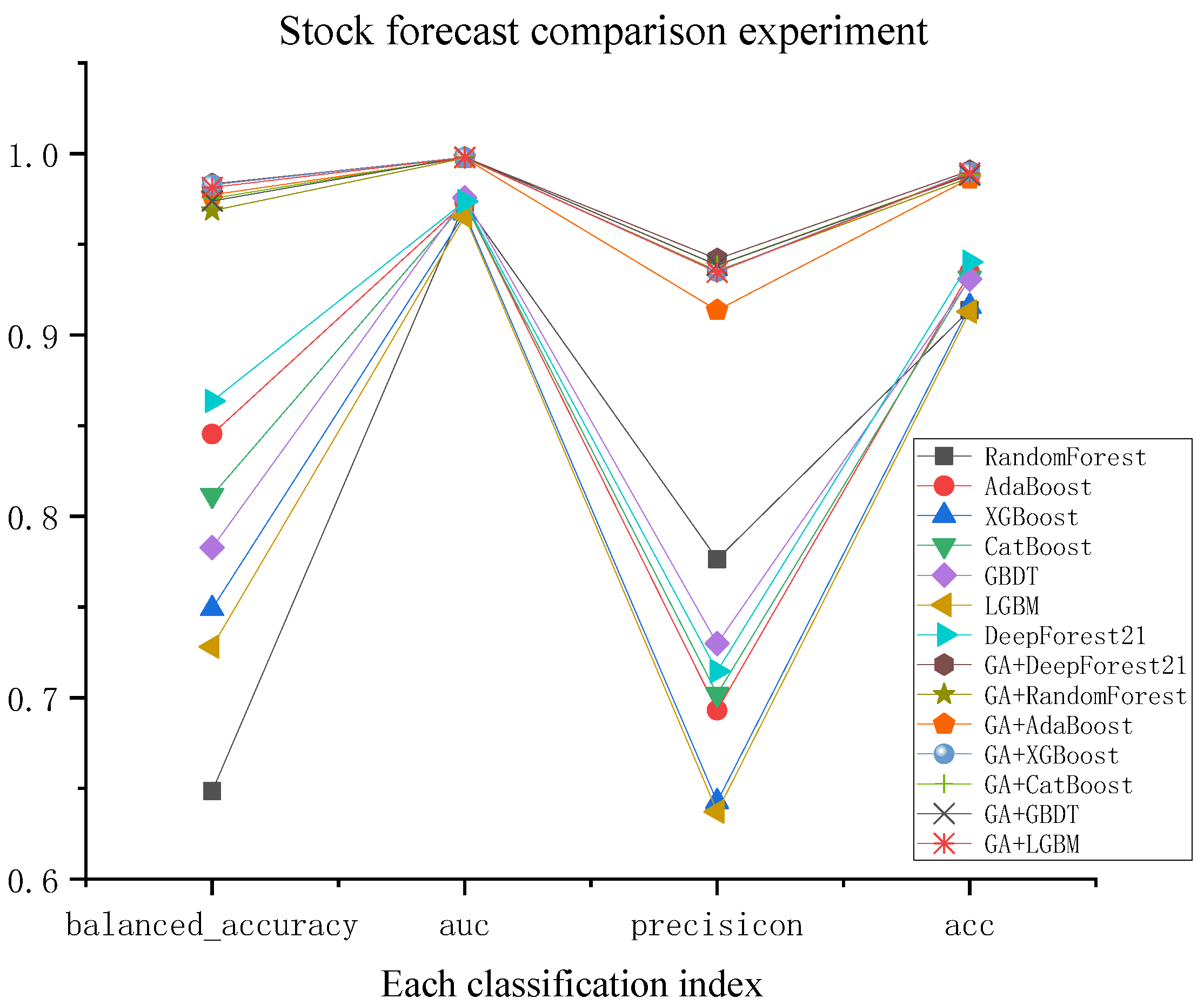
4.2. HSD Forecast Results

As shown in Table 5, under the same experimental environment settings, there is a considerable improvement in the experimental results after multi-layer GA feature selection model screening compared with featureless selection. The featureless selection data are filled with many features that affect the model decision, and the performance of each model also affects its fitting performance to the data. The mean values of all the compared models on the balanced accuracy, AUC, precision, recall, f1_score and acc metrics are 0.7756, 0.9715, 0.6994, 0.5830, 0.6234 and 0.9256. After the multi-layer GA feature selection, the mean values of evaluation metrics on each model were 0.9775, 0.9978, 0.9339, 0.9635, 0.9484 and 0.9883, and the fitting ability of each model to the data was significantly improved.
As shown in Figure 8, after multilayer GA feature selection, the important feature data outperformed the full-dimensional feature data on each model. For the data without multilayer GA feature selection, the imbalance problem and the influence of redundant features in the HSD data set make each model’s balanced accuracy and precision performance poorer. The performance of the model itself and its ability to fit the data directly responds to the performance of each index, such as RF, XGB and LGBM, and cannot fit these data well compared with other models. The RF with the Bagging method performs much lower than the other models with the Boosting method in terms of balanced accuracy, which may be due to the fact that the parallel, put-back sampling method of Bagging does not cope well with a large number of redundant features and extreme imbalance problems present in the HSD data set. In contrast, the model by the Boosting method performs better on each metric because it adjusts the sample weights according to the training results, giving higher weights to the samples with wrong decisions [23]. However, RF can cope well with high-latitude data sets [24], making its performance in precision better than other models.
However, after two-dimensionality reductions by multilayer GA feature selection, the performance of each model is significantly improved and stable due to further elimination of relatively redundant features; the balancing accuracy and precision especially have greatly improved. In summary, this proves that the model proposed in this paper can effectively reduce the dimensionality of the HSD features and significantly improve the model’s prediction performance by eliminating the features that are still relatively redundant after dimensionality reduction. The significant increase and stabilization in the precision index in the figure further prove that the feature selection model of this paper is effective in redundant denoising features.

5. Discussion

Figure 9 shows the distribution of the samples in the HSD data set, with positive samples indicating that the company implemented an HSD in the current year and negative samples indicating that the company did not implement an HSD in the current year. The distribution of positive and negative samples in the training and test sets is different, and each company implemented 3, 161 stock dividends in the training set in seven years. However, the number of non-implemented dividends far exceeds that of implemented dividends, with a ratio of about 6.7:1. In the test set, 383 companies implemented stock dividends in the eighth year, and the remaining 3083 companies did not implement high dividends, with a ratio of about 8:1. Therefore, the ratio of positive and negative samples in the training set is different from that in the test set. Therefore, the ratio of positive and negative samples in the training set differs significantly from those of positive and negative samples in the test set.
Figure 10 shows the balanced accuracy performance of the models on the training set and test sets, which have noticeable differences. Five models show good performance on the test set after training, among which LGBM, AdaB, XGB and RF have a significant difference in performance between the training and test sets, and the difference between the performance of RF on the training and test sets reaches 0.02. GBDT has a minor improvement after training, and the difference between the performance of balanced accuracy on the test and training sets is less than 0.005. CatB is different from other models in that its performance in the test set does not improve after training compared to the training set. Therefore, the LGBM classification model is constructed by adversarial validation to check whether the training and test set distributions are consistent, creating a new label column with test set samples labelled with 1 and training set samples labelled with 0, and predicting the probability that the sample is in the training or test set. Suppose the model performs well enough on the AUC. In that case, it can indicate that the classifier can excel in classifying samples from either the training set or the test set, i.e., it indicates a significant difference in the distribution of the training and test sets.
Figure 11 shows the experimental results of the adversarial validation. The AUC is 0.96, which indicates that the model can more clearly identify whether the samples come from the training set or the test set, further proving that there is a significant difference between the training set and the test set, i.e., the distribution is unbalanced. Therefore, the inconsistent distribution of samples brings about a balanced accuracy gap between the training set and the test set.

6. Conclusions and Prospects

In order to carry out HSD prediction, starting from the features affecting HSD, a feature selection model based on multilayer GA is proposed to eliminate the still relatively redundant feature based on dimensionality reduction and the comparison before and after feature selection is verified on seven ensemble models. The experiments show that this model can effectively reduce the dimensionality of the HSD feature, can eliminate the still relatively redundant feature after the dimensionality reduction and can improve the performance of the six evaluation indicators on the seven prediction models and predict the HSD more accurately. Finally, the impact of the inconsistent distribution of the HSD data set on the model balance accuracy was analyzed through confrontation validation. The main ideas of this model are as follows.
(1)
When using the ensemble learning model and TSCV metrics as the fitness function, the ensemble model’s excellent performance enables the genetic algorithm’s fitness value to reach convergence with a small number of iterations. For data sets with large data dimensions, this approach can save time by setting a smaller number of iterations to reach convergence quickly, but how to determine the exact number of iterations is something worth exploring further.
(2)
For the two-dimensionality reduction processes of the model, corresponding adaptation functions are set in each layer according to the changes in data dimensionality and the unbalanced characteristics of the HSD data set.
(3)
According to the HSD data set’s time-series characteristics, the HSD’s TSCV is introduced.
(4)
The TSCV indicator in the ensemble model is used as the fitness function, which not only takes into account the time-series characteristics of the HSD data set but also avoids overfitting while evaluating the model effect of the data in the feature contained in the selected populations in GA.
Future extensions will focus on the following three aspects:
(1)
Given the excellent performance of the ensemble learning model, when combined with the GA, only a small number of iterations are required for the fitness to reach convergence, and how to determine the appropriate number of iterations is worth exploring further.
(2)
The genetic algorithm’s crossover rate and mutation rate can be set too large to enhance the searchability of the algorithm, making the chromosomes in the population more diverse. The combination of features is more abundant but leads to an optimal solution in the combination of features that cannot be fixed. Too low a crossover and mutation rate can easily make the genetic algorithm fall into local optimum and reduce the searchability of the algorithm. The focus of the subsequent research is how to set the appropriate crossover and mutation rate.
(3)
There is a serious imbalance problem in the HSD data set. However, it also has very distinctive time-series characteristics, and the eight-year data limit further study of the HSD phenomenon, so the traditional methods of dealing with imbalance, such as SMOTE, cannot cope with this problem well. The focus of the subsequent work is on how to better solve the imbalance problem of data sets with time-series characteristics or collect more data on HSDs.

Author Contributions

Conceptualization, X.L.; methodology, X.L.; validation, X.L. and Q.Y.; formal analysis, X.L.; investigation, Q.Y.; resources, Q.Y.; data curation, X.L.; writing—original draft preparation, X.L.; writing—review and editing, X.L.; visualization, X.L.; supervision, C.T., Z.L. and Y.Y.; project administration, X.L.; funding acquisition, Q.Y. All authors have read and agreed to the published version of the manuscript.

Funding

This research was funded by the National Natural Science Foundation of China (Grant Nos.62062001), the Ningxia first-class discipline and scientific research projects (electronic science and technology, NXYLXK2017A07), the Provincial Natural Science Foundation of NingXia (NZ17111.2020AAC03219), and the Research Platform of North Minzu University(Digital Agriculture Enabling Ningxia Rural Revitalization Innovation Team).

Institutional Review Board Statement

Not applicable.

Informed Consent Statement

Not applicable.

Data Availability Statement

Some or all data, models or code generated or used during the study are available from the corresponding author on request.

Acknowledgments

This article would not have been possible without the valuable reference materials that I received from my supervisor, whose insightful guidance and enthusiastic encouragement in the course of my shaping this article definitely gain my deepest gratitude.

Conflicts of Interest

The authors declare no conflict of interest.

References

  1. Li, X.D.; Yu, H.H.; Lu, R.; Xu, L.B. Research on the Phenomenon of “highly dividend” in Chinese Stock Market. Manag. World 2014, 11, 133–145. [Google Scholar]
  2. Wang, Y. Analysis on the influencing factors of highly dividend of listed companies. Chin. Foreign Entrep. 2019, 29, 1. [Google Scholar]
  3. Feng, X.X. Listed companies “highly dividend” is high return or interest delivery? J. Financ. Account. 2018, 17, 74–78. [Google Scholar]
  4. Chen, X.; Chen, X.Y.; Ni, F. An empirical study on the signaling effect of initial dividends of listed companies in China. Econ. Sci. 1998, 5, 34–44. [Google Scholar] [CrossRef]
  5. Gong, H.Y. A study on the behavior of dividend conversions of listed companies in China based on dividend catering theory. Shanghai Financ. 2010, 11, 67–72. [Google Scholar]
  6. Yan, J.X. Research on “Highly Dividend” Excess Returns of Gem Listed Companies and Its Influencing Factors. Master’s Thesis, Soochow University, Jiangsu, China, 2017. [Google Scholar]
  7. Ling, S.Q.; Xie, C. High dividend to an investment strategy based on the Logit model. J. Time Financ. 2017, 20, 277–281. [Google Scholar]
  8. Yan, M.C. Investment Strategy Analysis Based on the Effect of “Highly Dividend and Transfer” Announcement. Master’s Thesis, Nanjing Agricultural University, Nanjing, China, 2017. [Google Scholar]
  9. Jiang, C.; Xia, X.L.; Wu, W.; Cui, H.B.; Ma, C.X. Research on highly dividend prediction of listed companies based on Data Mining. J. Hubei Univ. 2021, 43, 698–705. [Google Scholar]
  10. Mai, J.F.; Zhao, H.Q. Research on the prediction of “highly dividend” of Chinese listed companies: Based on the mixed analysis of Grey Prediction and Support Vector Regression Model. J. Shaoguan Univ. 2001, 42, 5–10. [Google Scholar]
  11. Zhang, T.H.; Luo, K.X. An empirical study on highly dividend prediction of listed companies based on ensemble learning. J. Comput. Eng. Appl. 2022, 58, 255–262. [Google Scholar]
  12. Yu, Q.D.; Dai, J.J. Prediction of highly dividend of listed companies based on Combination Model. Math. Theory Appl. 2020, 40, 101. [Google Scholar]
  13. Cao, L.; Li, J.; Zhou, Y.; Liu, Y.; Liu, H. Automatic feature group combination selection method based on GA for the functional regions clustering in DBS. Comput. Methods Programs Biomed. 2020, 183, 105091. [Google Scholar] [CrossRef] [PubMed]
  14. Saibene, A.; Gasparini, F. GA for feature selection of EEG heterogeneous data. arXiv 2021, arXiv:2103.07117, 2021. [Google Scholar]
  15. Li, X.H.; Jia, H.D.; Cheng, X.; Li, T. Prediction of Stock market volatility based on Improved Genetic Algorithm and Graph Neural Network. J. Comput. Appl. 2022, 42, 1624–1633. [Google Scholar]
  16. Elsawy, A.; Selim, M.M.; Sobhy, M. A hybridised feature selection approach in molecular classification using CSO and GA. Int. J. Comput. Appl. Technol. 2019, 59, 165–174. [Google Scholar] [CrossRef]
  17. Omidvar, M.; Zahedi, A.; Bakhshi, H. EEG signal processing for epilepsy seizure detection using 5-level Db4 discrete wavelet transform, GA-based feature selection and ANN/SVM classifiers. J. Ambient. Intell. Humaniz. Comput. 2021, 12, 10395–10403. [Google Scholar] [CrossRef]
  18. Mandal, R.; Azam, B.; Verma, B.; Zhang, M. Deep Learning Model with GA-based Visual Feature Selection and Context Integration. In Proceedings of the 2021 IEEE Congress on Evolutionary Computation (CEC), Kraków, Poland, 28 June–1 July 2021; pp. 288–295. [Google Scholar]
  19. Zhang, Y.; Wang, X.N. Text Feature Selection Method based on Word2Vec Word Embedding and Genetic Algorithm for High-dimensional Biological Gene Selection. Comput. Appl. 2021, 41, 3151–3155. [Google Scholar]
  20. Chen, Q.R.; Li, Y.L.; Xu, K.Q.; Liu, X.L.; Wang, S.Q. WKNN Feature Selection Method based on Self-tuning adaptive Genetic Algorithm. Comput. Eng. Appl. 2021, 57, 164–171. [Google Scholar]
  21. Xie, L.R.; Yang, H.; Li, J.W. Bearing Fault Diagnosis of Doubly-Fed Wind Turbine Based on Ga-ENN Feature Selection and Parameter Optimization. J. Sol. Energy 2021, 42, 149–156. [Google Scholar]
  22. Zhou, Z.H.; Feng, J. Deep forest. Natl. Sci. Rev. 2019, 6, 74–86. [Google Scholar] [CrossRef] [PubMed]
  23. Bühlmann, P. Bagging, boosting and ensemble methods. In Handbook of Computational Statistics; Springer: Berlin/Heidelberg, Germany, 2012; pp. 985–1022. [Google Scholar]
  24. Breiman, L. Random forests. Mach. Learn. 2001, 45, 5–32. [Google Scholar] [CrossRef] [Green Version]
Figure 1. Multilayer GA feature selection model.
Symmetry 14 01415 g001
Figure 2. TSCV for HSD setting.
Symmetry 14 01415 g002
Figure 3. GA combined with TSCV_AUC of each model.
Symmetry 14 01415 g003
Figure 4. GA combined with TSCV_ACC of each model.
Symmetry 14 01415 g004
Figure 5. The optimal solution encoding.
Symmetry 14 01415 g005
Figure 6. Convergence of fitness of optimal solution.
Symmetry 14 01415 g006
Figure 7. Coding of optimal solution after dimensionality reduction.
Symmetry 14 01415 g007
Figure 8. Comparison of model effects.
Symmetry 14 01415 g008
Figure 9. HSD data set distribution.
Symmetry 14 01415 g009
Figure 10. Balanced accuracy difference between training and test set.
Symmetry 14 01415 g010
Figure 11. AUC against validation experiments.
Symmetry 14 01415 g011
Table 1. Data set Overview.
Data CategoriesNumber of FeaturesNumber of RowsNotes
Basic Data43466
Training set Yearly data36224,262First seven years of data
Test set Yearly data36234668th year data
Training set Daily data615,899,132First seven years of data
Test set Daily data61842,2388th year data
Table 2. GA parameter setting.
ModelData SetFitness FunctionNumber of PopulationsNumber of IterationsCrossover RateMutation Rate
First layerTraining setsModel: TSCV_ACC, AUC20050.70.5
Second layerTraining setsModel: TSCV_AUC500200.30.1
Third layerOptimal solution data setModel: TSCV_balanced accuracy20050.30.1
Fourth layerOptimal solution data setModel: TSCV_balanced accuracy500200.30.1
Table 3. Parameter setting of each ensemble learning model.
ModelParameter Setting
RandomForestn_estimators = 400, max_depth = 13, min_samples_leaf = 10, min_samples_split = 30
AdaBoostn_estimators = 800, learning_rate = 0.1
XGBoostn_estimators = 400, learning_rate = 0.07, max_depth = 7, min_child_weight = 1
CatBoostlearning_rate = 0.1, iterations = 400, max_depth = 5
GBDTlearning_rate = 0.01, max_depth = 11, n_estimators = 850, subsample = 0.8, random_state = 5, min_samples_split = 100, min_samples_leaf = 20
LGBMn_estimators = 800, learning_rate = 0.03, max_depth = 13, num_leaves = 50, max_min = 225, min_data_in_leaf = 31
DF21n_bins = 255, n_trees = 100, max_layers = 20
Table 4. The optimal solution after dimensionality reduction.
CategoriesFeatures
Basic features (12 in total)Net interest expense, total equity attributable to owners of the parent company, highest price, lowest price, transaction amount, earnings before interest, taxes, depreciation and amortization, undistributed earnings, cash received from sales of goods and services, various taxes and fees paid, cash paid for investments, effect of exchange rate changes on cash and cash equivalents, ending balance of cash and cash equivalents
Statistical features
(12 in total)
Return on net assets (diluted, %), Tangible net assets/total assets (%), Capital fixation rate (%), 120-day Sharpe ratio, Same necessary growth in total operating (%), Same necessary growth in return on net assets (diluted) (%), Total fixed assets turnover (times) Operating profit/total liabilities Money capital/Interest-bearing current liabilities Net non-financing cash flow/current liabilities Long-term amortization expense/total assets (%) P/E ratio
Individual stock features (7 in total)Operating income per share (RMB/share), capital surplus per share (RMB/share), total operating income per share, net cash flow per share, basic earnings per share, and net cash flow from operating activities per share increased by the same amount (%), and net cash flow from operating activities per share increased by the same amount (%) Transfers per share
Table 5. Comparison of experimental model effects.
EvaluationModels
RFGA-
RF
AdaBoostGA-AdaBXGBoostGA-
XGB
CatBoostGA-
CatB
GBDTGA-
GBDT
LGBMGA-
LGBM
DF21GA-
DF21
balanced_acc0.64850.96850.84540.97740.74910.98270.81160.97520.78270.97390.72810.98140.86350.9832
auc0.97280.99760.97290.99740.96710.99790.97280.99810.97570.99810.96550.99780.97360.9980
precisicon0.77630.93540.69310.91360.64260.93480.70200.93860.72990.93850.63720.93470.71450.9419
recall0.30810.94520.73120.96610.53530.97390.65800.95820.59270.95560.49090.97130.76500.9739
f1_score0.44110.94030.71160.93910.58410.95400.67920.94830.65420.94700.55450.95260.73900.9576
acc0.91370.98670.93450.98520.91580.98960.93130.98850.93080.98820.91290.98930.94030.9905
Publisher’s Note: MDPI stays neutral with regard to jurisdictional claims in published maps and institutional affiliations.

