Harmonic Balance Method to Analyze the Steady-State Response of a Controlled Mass-Damper-Spring Model

Abstract

This research is concerned with extracting the approximate solutions of a controlled mass-damper-spring model via the harmonic balance method. The stability of these solutions was checked with the aid of Floquet theory. A nonlinear saturation controller (NSC), a linear variable differential transformer (LVDT) and a servo-controlled linear actuator (SCLA), were applied to suppress the undesired oscillations of the harmonically-excited car. 2D and 3D graphical plots are included based upon the equations resulting from the harmonic balance method. Moreover, a numerical simulation was established using the fourth order Rung–Kutta technique in order to confirm the overall controlled behavior of the studied model.

1. Introduction

Mass-damper-spring models are considered basic representations for many industrial applications. They usually represent vehicle suspension mechanisms that are very important to control in order to provide comfort and safety to passengers. They can also represent the mechanisms of robotic arms to be controlled for specific tasks. They are often modelled by second-order linear or nonlinear differential equations. With the use of linear differential equations, the exact solution can be extracted via theorems based on calculus. However, in cases of nonlinear differential equations the exact solution cannot be reached, leading researchers to seek approximate solutions. There are several methods that give the asymptotic approximate solution, with some assumptions in order to maintain the validity of the method. One important method among these is the harmonic balance method. Hamdan and Burton [1] investigated the steady-state periodic response and stability of a softening Duffing oscillator. They showed that the qualitative nature of the harmonic balance solution could change if two harmonics were used instead of one in the approximate solution. Hassan [2] determined firstly the approximate solution for the steady-state periodic response of a nonlinear oscillator, and then the local stability of the solution by checking the linearization around the predicted solution. Hamdan and Shabaneh [3] compared approximate solutions achieved by the one-term harmonic balance method, the two-term harmonic balance method, and the two-term time transformation method for the large amplitude free vibration of a strongly nonlinear oscillator. Maccari [4] balanced the harmonic terms in order to analyze the response of a periodically-excited mass point moving along a parabola. Al-Qaisia and Hamdan [5] studied the local stability and response of a harmonically-excited slender cantilever beam that was partially immersed in a fluid. Dunne [6] utilized a split frequency in the harmonic balance method in order to analyze the sub-harmonic responses of a periodically-excited oscillator, and included many solution harmonics to generate high-accuracy periodic solutions. Malatkar and Nayfeh [7] studied a harmonically-excited combination of a linear sub-system coupled to a nonlinear oscillator where cyclic-fold, Hopf, symmetry-breaking, and period-doubling bifurcations were present. Zhang et al. [8] suppressed the resonant vibrations of a nonlinear dynamical system by applying a transmissibility system with a nonlinear damping element. Carrella et al. [9] focused on the transmissibility force of a quasi-zero-stiffness isolator which consisted of vertical and oblique springs whose stiffness exhibited linear, pre-stress linear, or pre-stress nonlinear softening. Gatti et al. [10] modelled a single-degree-of-freedom shaker which drove a nonlinear-hardening dynamical system and analyzed the overall dynamic behavior of the combination. Nayfeh and Nayfeh [11] examined the dynamics and stability (local and global) of a cutting tool on a lathe via the methods of multiple sales, harmonic balance, and Floquet theory. Luo and O’Connor [12] utilized the harmonic balance method in order to study the stable and unstable periodic motions in the Mathieu–Duffing equation. Le and Ahn [13] isolated vibrations with a negative stiffness structure for driver seats in a vehicle with low-frequency vibration conditions. Ji and Zhang [14,15,16,17] studied the primary, super-harmonic, sub-harmonic, and additive resonances of a hardly-excited time-delayed nonlinear oscillator, using the center manifold and multiple scales methods. They also found that changing the initial conditions could create bi-stable periodic solutions, and the primary resonance vibrations could be suppressed by about 88%. Kamel et al. [18,19] extracted multiple-scale approximate solutions of a nonlinear differential equation governing the motion of a magnetically-suspended mass controlled by a saturation controller in case of absent and present time delay. Hao and Cao [20] isolated the vibrations of a nonlinear oscillator with quasi-zero-stiffness modelled by three springs (two horizontal and one vertical). El-Sayed and Bauomy [21] focused on controlling the vibrational motion of a 2DOF dynamical system excited by multi-parametric forces via a nonlinear absorber at severe subharmonic and internal resonances. Motallebi et al. [22] used the harmonic balance method in order to investigate the nonlinear phenomena (jump and bifurcation) of a cantilever beam with geometric nonlinearity. Perez-Molina et al. [23] studied the actuation of a closed cylinder with a mobile piston, using a spring-damper combination which generated a control force in order to compensate the effect of high pressure nitrogen. Zhou et al. [24] modelled a periodically-excited quarter-car including a nonlinear damper-spring, where its dynamical behavior was analyzed via the Newmark and incremental harmonic balance methods. Kandil and Eissa [25,26] proposed an improved positive position feedback controller, with a pair of saturation controllers coupled at each peak of the conventional controller. They investigated the dynamical response in cases of zero-time delay, or significant time delay. Silveira et al. [27] studied the effect of non-symmetrical damping on the suspension process of transport vehicles and how this affected passenger comfort. Kandil et al. [28,29] tried to couple a saturation controller to a rotating blade that operated in a super-sonic gas flow. They examined the time delay effects on the control process and determined a measure for the safe ranges of the applied time delays. Zhou et al. [30] utilized the incremental harmonic balance method for analyzing a vehicle’s dynamic system behavior by quadratic and cubic nonlinearities. Kandil et al. [31,32] discussed adapting the performance of positive position feedback and nonlinear saturation controllers by acquiring the rotor speed in an active magnetic bearings model. Uemori et al. [33] measured stiffness and fluctuations in a cantilever beam by exploring the shifts in its Eigen frequency and coupling a secondary resonator to the primary system, i.e., the beam. With 2D and 3D plots, Kandil et al. [34] analyzed the dynamical behavior of a mass-damper-spring model under the control of a servo-controlled linear actuator. They adopted the Krylov–Bogoliubov averaging method in order to extract the amplitude-phase equations of the controlled model.

This current research deals with a controlled mass-damper-spring model, equations of which were solved via the harmonic balance method. The resulting solutions were tested for stability with the aid of Floquet theory. Then, 2D and 3D graphical plots were included based upon the equations resulted from the harmonic balance method. Moreover, a numerical simulation was carried out using the fourth order Rung–Kutta technique to confirm the overall controlled behavior of the studied model.

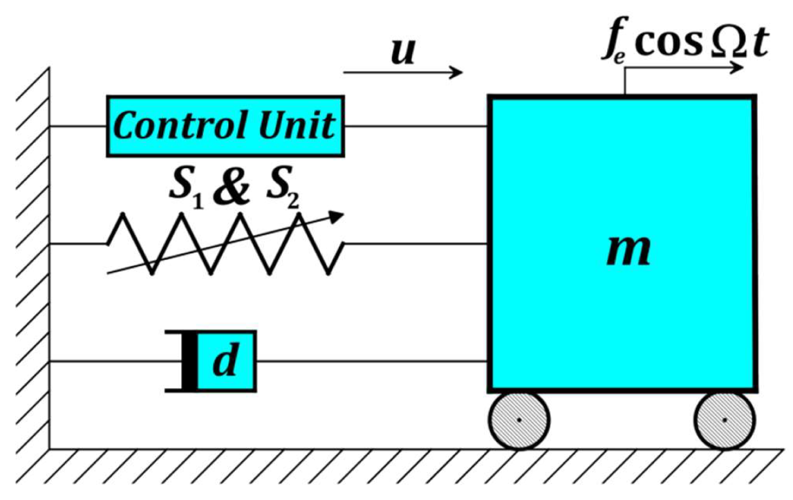
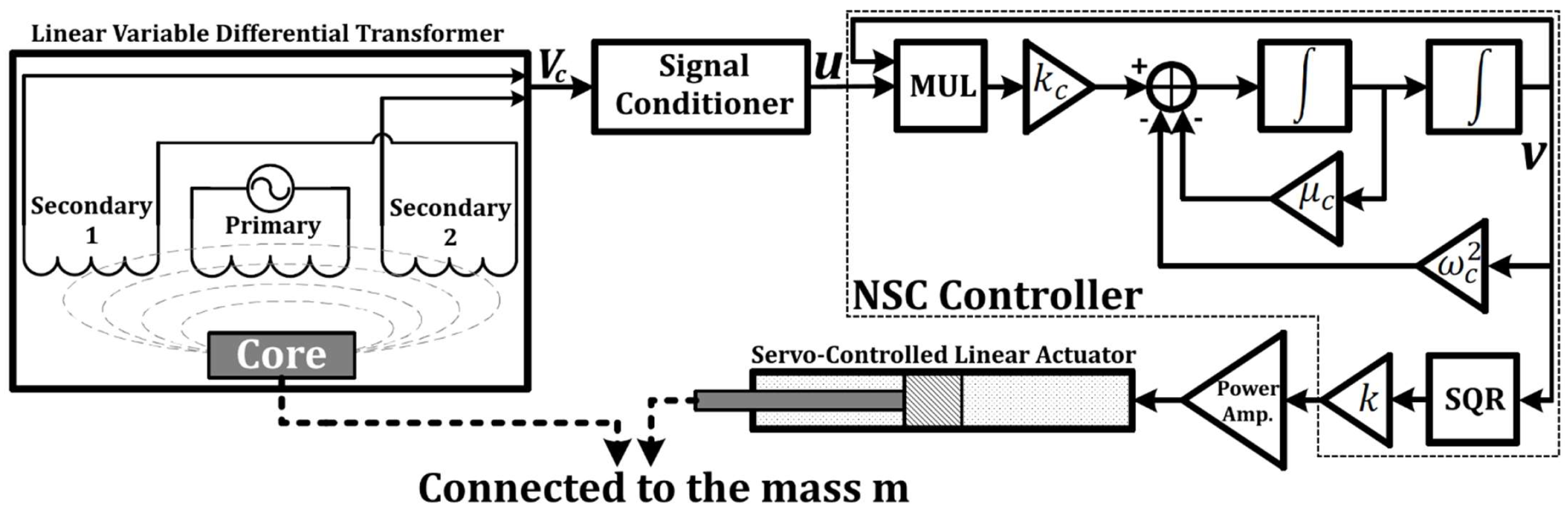
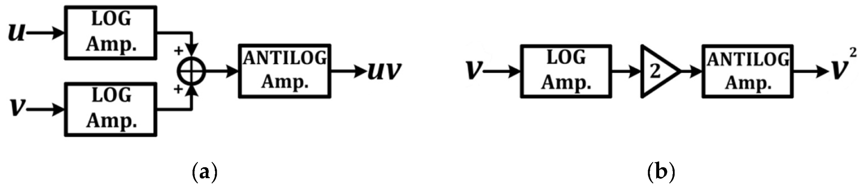
2. System Modelling and Harmonic Balance Method

A proto-type car of mass $m$ was connected to a stationary surface by a dashpot (of viscosity $d$), a nonlinear spring (of stiffness $S_1\&S_2$), and a control unit as shown in Figure 1. The car’s motion was excited by a harmonic force $f_e\cos \left(\mathsf{\Omega }t\right)$. Applying Newton’s second law of motion ($ma=\mathsf{\Sigma }F$) can give us the dynamical equation of the car’s displacement $u$ as follows

$$m\ddot{u}=-d\dot{u}-S_{1}u-S_2{u}^3+f_e\cos \left(\mathsf{\Omega }t\right)+F_c\Rightarrow m\ddot{u}+d\dot{u}+S_{1}u+S_2{u}^3=f_e\cos \left(\mathsf{\Omega }t\right)+F_c$$

(1)

where $F_c$ is a control force generated by the control unit shown in the figure above. The implementation of this control unit is shown in Figure 2, with the car’s position sensed by an LVDT (linear variable differential transformer). Its output voltage $V_c$ is proportional to the car’s displacement $u$. Then, a signal conditioner is utilized for adjusting a suitable signal to be provided to the NSC controller whose model equation is known to be:

$$\ddot{v}+{\mu }_c\dot{v}+{\omega }_c^{2}v=k_{c}uv$$

(2)

where $v$ is the output control signal, ${\mu }_c$ is the NSC’s damping factor, ${\omega }_c$ is its natural frequency, and $k_c$ is its gain of feedback. The control signal $v$ is computed based on Equation (2) as shown in Figure 2, then be amplified by $k$ (the control gain) to produce the control force $F_c=k{v}^2$. The power amplifier’s role is to supply the SCLA (servo-controlled linear actuator) with a drive current proportional to $F_c$. This SCLA can modify the car’s position in order to mitigate unwanted oscillations. A brief description of both multiplier (MUL) and squarer (SQR) units is given in Figure 3. As seen in Figure 3a, the MUL unit can be implemented by inserting both $u$ and $v$ signals into LOG amplifiers whose outputs are $\log u$ and $\log v$, respectively. Through summing point, its output is $\log u+\log v=\log uv$. Then, the result is inserted into an ANTILOG amplifier whose output is ${\log }^{-1}\left[\log uv\right]=uv$. In Figure 3b, the SQR unit can be designed by inserting the $v$ signal into a LOG amplifier to produce $\log v$. The result can be amplified by a gain of $2$ to become $2\log v=\log v^2$. Then, the LOG can be eliminated via an ANTILOG amplifier which generates ${\log }^{-1}\left[\log v^2\right]=v^2$. The LOG and ANTILOG amplifiers circuits can be designed using operational amplifiers, resistors and diodes with the help of any industrial electronics textbook.

Collecting and simplifying Equations (1) and (2) gives

$$\ddot{u}+\mu \dot{u}+{\omega }^{2}u+\alpha u^3=f\cos \left(\mathsf{\Omega }t\right)+k{v}^2$$

(3a)

$$\ddot{v}+{\mu }_c\dot{v}+{\omega }_c^{2}v=k_{c}uv$$

(3b)

where $\mu =d/m$, ${\omega }^2=S_1/m$, $\alpha =S_2/m$, $f=f_e/m$, $k^{*}=k/m$, while we have eliminated the asterisk in $k^{*}$ for simplicity. The method of harmonic balance can be adopted for solving the above system of nonlinear differential equations. Thus, we substitute harmonic steady-state solutions in a Fourier series form [35,36]:

$$u=u_0={\displaystyle \sum }_{n=1}^{\infty }\left[A_n\cos \left(n\mathsf{\Omega }t\right)+B_n\sin \left(n\mathsf{\Omega }t\right)\right]\cong A_1\cos \left(\mathsf{\Omega }t\right)+B_1\sin \left(\mathsf{\Omega }t\right)$$

(4a)

$$v=v_0={\displaystyle \sum }_{n=1}^{\infty }\left[P_n\cos \left(\frac{n\mathsf{\Omega }t}{2}\right)+Q_n\sin \left(\frac{n\mathsf{\Omega }t}{2}\right)\right]\cong P_1\cos \left(\frac{\mathsf{\Omega }t}{2}\right)+Q_1\sin \left(\frac{\mathsf{\Omega }t}{2}\right)$$

(4b)

into Equation (3) and obtain

$$\begin{gathered} \left[\left({\omega }^2-{\mathsf{\Omega }}^2\right)A_1+\frac{3\alpha }{4}\left(A_1^3+A_1{B}_1^2\right)+\mu \mathsf{\Omega }{B}_1\right]\cos \left(\mathsf{\Omega }t\right)+\left[\left({\omega }^2-{\mathsf{\Omega }}^2\right)B_1+\frac{3\alpha }{4}\left(B_1^3+A_1^2{B}_1\right)-\mu \mathsf{\Omega }{A}_1\right]\sin \left(\mathsf{\Omega }t\right) \\ =\frac{k}{2}\left(P_1^2+Q_1^2\right)+\left[f+\frac{k}{2}\left(P_1^2-Q_1^2\right)\right]\cos \left(\mathsf{\Omega }t\right)+k{P}_1{Q}_1\sin \left(\mathsf{\Omega }t\right)+HOH \end{gathered}$$

(5a)

$$\begin{gathered} \left[\left({\omega }_c^2-\frac{{\mathsf{\Omega }}^2}{4}\right)P_1+\frac{{\mu }_c\mathsf{\Omega }}{2}{Q}_1\right]\cos \left(\frac{\mathsf{\Omega }t}{2}\right)+\left[\left({\omega }_c^2-\frac{{\mathsf{\Omega }}^2}{4}\right)Q_1-\frac{{\mu }_c\mathsf{\Omega }}{2}{P}_1\right]\sin \left(\frac{\mathsf{\Omega }t}{2}\right) \\ =\left[\frac{k_c}{2}\left(A_1{P}_1+B_1{Q}_1\right)\right]\cos \left(\frac{\mathsf{\Omega }t}{2}\right)+\left[\frac{k_c}{2}\left(B_1{P}_1-A_1{Q}_1\right)\right]\sin \left(\frac{\mathsf{\Omega }t}{2}\right)+HOH \end{gathered}$$

(5b)

where the $HOH$ stands for the higher-order harmonics that are not necessary in this analysis. We require the first-order harmonic, in order to obtain the first-order approximate solution which is sufficient for analyzing the system dynamics. In future work, we can deal with higher-order harmonics to get higher-order approximate solutions. Express $A_1$, $B_1$, $P_1$, and $Q_1$ in the polar form as follows:

$$A_1+i{B}_1=a{e}^{i\theta }=a\left(\cos \theta +i\sin \theta \right)$$

(6a)

$$P_1+i{Q}_1=b{e}^{i\varphi }=b\left(\cos \varphi +i\sin \varphi \right)$$

(6b)

where {$a$, $b$} and {$\theta$, $\varphi$} are the amplitudes and phases of the mass and the controller, respectively. Substituting Equation (6) into Equation (5), then equalizing the coefficients of $\cos \left(\mathsf{\Omega }t\right)$, $\sin \left(\mathsf{\Omega }t\right)$, $\cos \left(\frac{\mathsf{\Omega }t}{2}\right)$, $\sin \left(\frac{\mathsf{\Omega }t}{2}\right)$ on both sides of Equation (5) can lead to the following:

$$\left({\omega }^2-{\mathsf{\Omega }}^2\right)a\cos \theta +\frac{3\alpha }{4}{a}^3\cos \theta +\mu \mathsf{\Omega }a\sin \theta -\frac{k}{2}{b}^2\cos \left(2\varphi \right)-f=0$$

(7a)

$$\left({\omega }^2-{\mathsf{\Omega }}^2\right)a\sin \theta +\frac{3\alpha }{4}{a}^3\sin \theta -\mu \mathsf{\Omega }a\cos \theta -\frac{k}{2}{b}^2\sin \left(2\varphi \right)=0$$

(7b)

$$\left({\omega }_c^2-\frac{{\mathsf{\Omega }}^2}{4}\right)b\cos \varphi +\frac{{\mu }_c\mathsf{\Omega }}{2}b\sin \varphi -\frac{k_c}{2}ab\cos \left(\theta -\varphi \right)=0$$

(7c)

$$\left({\omega }_c^2-\frac{{\mathsf{\Omega }}^2}{4}\right)b\sin \varphi -\frac{{\mu }_c\mathsf{\Omega }}{2}b\cos \varphi -\frac{k_c}{2}ab\sin \left(\theta -\varphi \right)=0$$

(7d)

Manipulating Equation (7) algebraically and simplifying:

$$\mu \mathsf{\Omega }a-\frac{k}{2}{b}^2\sin \left(\theta -2\varphi \right)-f\sin \theta =0$$

(8a)

$$\left({\omega }^2-{\mathsf{\Omega }}^2\right)a+\frac{3\alpha }{4}{a}^3-\frac{k}{2}{b}^2\cos \left(\theta -2\varphi \right)-f\cos \theta =0$$

(8b)

$$\frac{{\mu }_c\mathsf{\Omega }}{2}b+\frac{k_c}{2}ab\sin \left(\theta -2\varphi \right)=0$$

(8c)

$$\left({\omega }_c^2-\frac{{\mathsf{\Omega }}^2}{4}\right)b-\frac{k_c}{2}ab\cos \left(\theta -2\varphi \right)=0$$

(8d)

In case the controller is active such that $b\ne 0$, Equation (8c,d) can be solved to give us the steady-state amplitude $a$ of the mass in terms of the frequency $\mathsf{\Omega }$

$$a=\frac{1}{k_c}\sqrt{{\mu }_c^2{\mathsf{\Omega }}^2+4{\left({\omega }_c^2-\frac{{\mathsf{\Omega }}^2}{4}\right)}^2}=\psi$$

(9)

where $\psi$ is a function of $\mathsf{\Omega }$. Eliminating $\sin \left(\theta -2\varphi \right)$ from Equation (8a,c) and the same for $\cos \left(\theta -2\varphi \right)$ from Equation (8b,d) leads to the following:

$$\mu \mathsf{\Omega }{a}^2+\frac{k{\mu }_c\mathsf{\Omega }}{2k_c}{b}^2=fa\sin \theta$$

(10a)

$$\left({\omega }^2-{\mathsf{\Omega }}^2\right)a^2+\frac{3\alpha }{4}{a}^4-\frac{k}{k_c}\left({\omega }_c^2-\frac{{\mathsf{\Omega }}^2}{4}\right)b^2=fa\cos \theta$$

(10b)

To get rid of $\theta$, Equation (10) can be solved simultaneously which gives us a quartic equation in $b$:

$${\delta }_1{b}^4+{\delta }_2{b}^2+{\delta }_3=0$$

(11)

where

$$\begin{gathered} {\delta }_1=\frac{k^2}{4}{\psi }^2 \\ {\delta }_2=\frac{k}{k_c}\left[{\mu }_c\mu {\mathsf{\Omega }}^2{\psi }^2-2\left({\omega }_c^2-\frac{{\mathsf{\Omega }}^2}{4}\right)\left(\left({\omega }^2-{\mathsf{\Omega }}^2\right){\psi }^2+\frac{3\alpha }{4}{\psi }^4\right)\right] \\ {\delta }_3={\mu }^2{\mathsf{\Omega }}^2{\psi }^4+{\left[\left({\omega }^2-{\mathsf{\Omega }}^2\right){\psi }^2+\frac{3\alpha }{4}{\psi }^4\right]}^2-f^2{\psi }^2 \end{gathered}$$

Equation (11) can be solved as a quadratic equation in $b^2$ using the discriminant, and then the square root should be applied with a positive sign for gaining the real positive controller amplitude $b$ as

$$b=\sqrt{\frac{-{\delta }_2\pm \sqrt{{\delta }_2^2-4{\delta }_1{\delta }_3}}{2{\delta }_1}}$$

(12)

Once the steady-state amplitudes ($a$ and $b$) are calculated, their local stability are usually investigated by superposing small perturbations on both $u$ and $v$ steady-state solutions as

$$u=u_0+u_1$$

(13a)

$$v=v_0+v_1$$

(13b)

Substituting Equation (13) into Equation (3), with the fact that $u_0$ and $v_0$ satisfy Equation (3), and linearizing the resulting equation in $u_1$ and $v_1$, we can get

$${\ddot{u}}_1+\mu {\dot{u}}_1+{\omega }^2{u}_1+3\alpha u_0^2{u}_1=2k{v}_0{v}_1$$

(14a)

$${\ddot{v}}_1+{\mu }_c{\dot{v}}_1+{\omega }_c^2{v}_1=k_c\left[u_0{v}_1+v_0{u}_1\right]$$

(14b)

which is a system of equations with variable coefficients whose stability corresponds to the stability of the steady-state solutions $u_0=a\cos \left(\mathsf{\Omega }t-\theta \right)$ and $v_0=b\cos \left(\frac{\mathsf{\Omega }t}{2}-\varphi \right)$. Depending on Floquet theory [7,37], Equation (14) has solutions in the form

$$u_1\left(t\right)=e^{\gamma t}{\rho }_1\left(t\right)$$

(15a)

$$v_1\left(t\right)=e^{\gamma t}{\rho }_2\left(t\right)$$

(15b)

where $\gamma$ is the Floquet characteristic exponent, ${\rho }_1$ and ${\rho }_2$ are periodic functions whose periods are $T_1=2\pi /\mathsf{\Omega }$ and $T_2=4\pi /\mathsf{\Omega }$, respectively. Inserting Equation (15) into Equation (14) yields

$${\ddot{\rho }}_1+\left(2\gamma +\mu \right){\dot{\rho }}_1+\left({\gamma }^2+\mu \gamma +{\omega }^2+3\alpha u_0^2\right){\rho }_1=2k{v}_0{\rho }_2$$

(16a)

$${\ddot{\rho }}_2+\left(2\gamma +{\mu }_c\right){\dot{\rho }}_2+\left({\gamma }^2+{\mu }_c\gamma +{\omega }_c^2\right){\rho }_2=k_c\left[u_0{\rho }_2+v_0{\rho }_1\right]$$

(16b)

Equation (16) can be solved by expanding ${\rho }_i\left(t\right)$ into a Fourier series form like the way done in Equation (4). Thus, we suppose

$${\rho }_1={\displaystyle \sum }_{n=1}^{\infty }\left[G_n\cos \left(n\mathsf{\Omega }t\right)+H_n\sin \left(n\mathsf{\Omega }t\right)\right]\cong G_1\cos \left(\mathsf{\Omega }t\right)+H_1\sin \left(\mathsf{\Omega }t\right)$$

(17a)

$${\rho }_2={\displaystyle \sum }_{n=1}^{\infty }\left[M_n\cos \left(\frac{n\mathsf{\Omega }t}{2}\right)+N_n\sin \left(\frac{n\mathsf{\Omega }t}{2}\right)\right]\cong M_1\cos \left(\frac{\mathsf{\Omega }t}{2}\right)+N_1\sin \left(\frac{\mathsf{\Omega }t}{2}\right)$$

(17b)

Substituting Equation (17) into Equation (16), and then comparing the coefficients of $\cos \left(\mathsf{\Omega }t\right)$, $\sin \left(\mathsf{\Omega }t\right)$, $\cos \left(\frac{\mathsf{\Omega }t}{2}\right)$, $\sin \left(\frac{\mathsf{\Omega }t}{2}\right)$ on both sides can give us the following matrix equation:

$$\left[\begin{array}{cccc}{D}_{11}& D_{12}& D_{13}& D_{14}\\ D_{21}& D_{22}& D_{23}& D_{24}\\ D_{31}& D_{32}& D_{33}& D_{34}\\ D_{41}& D_{42}& D_{43}& D_{44}\end{array}\right]\left[\begin{array}{c}{G}_1\\ H_1\\ M_1\\ N_1\end{array}\right]=\left[\begin{array}{c}0\\ 0\\ 0\\ 0\end{array}\right]$$

(18)

where

$$\begin{array}{cc}{D}_{11}={\gamma }^2+{\omega }^2-{\mathsf{\Omega }}^2+\gamma \mu +\frac{3\alpha }{4}{a}^2\left[\cos \left(2\theta \right)+2\right]& D_{12}=2\gamma \mathsf{\Omega }+\mu \mathsf{\Omega }+\frac{3\alpha }{4}{a}^2\sin \left(2\theta \right)\\ D_{13}=-kb\cos \varphi & D_{14}=kb\sin \varphi \\ D_{21}=-D_{12}+\frac{3\alpha }{2}{a}^2\sin \left(2\theta \right)& D_{22}=D_{11}-\frac{3\alpha }{2}{a}^2\cos \left(2\theta \right)\\ D_{23}=-D_{14}& D_{24}=D_{13}\\ D_{31}=-\frac{k_c}{2}b\cos \varphi & D_{32}=-\frac{k_c}{2}b\sin \varphi \\ D_{33}={\gamma }^2+{\omega }_c^2-\frac{{\mathsf{\Omega }}^2}{4}+\gamma {\mu }_c-\frac{k_c}{2}a\cos \theta & D_{34}=\gamma \mathsf{\Omega }+\frac{{\mu }_c\mathsf{\Omega }}{2}-\frac{k_c}{2}a\sin \theta \\ D_{41}=-D_{32}& D_{42}=D_{31}\\ D_{43}=-D_{34}-k_{c}a\sin \theta & D_{44}=D_{33}+k_{c}a\cos \theta \end{array}$$

To obtain a characteristic equation governing $\gamma$, we can set the coefficient matrix determinant of Equation (18) equal to zero. If all $\gamma$ lie in the left half of Argand diagram, then the periodic solutions $u_0$ and $v_0$ will be asymptotically stable. Otherwise, they will be unstable.

3. Results and Discussion

Graphical plots (2D and 3D) are included here based upon the equations resulting from the harmonic balance method. The 2D plots contain either heavy-colored branches which refer to stable solutions, or light-colored branches which refer to unstable ones. This is the result of Floquet theory analysis. The 3D plots contain surfaces giving a generalized aspect of the 2D plots. The surface top is denoted by a dark red color, while its bottom is denoted by a dark blue color. The physical constants of the mass-damper-spring model were selected as: $m=10 \mathrm{kg}$, $d=0.2 {\mathrm{Nm}}^{-1}\mathrm{s}$, $S_1=100 {\mathrm{Nm}}^{-1}$, $S_2=8 {\mathrm{Nm}}^{-3}$, $f_e=0.6 \mathrm{N}$, and $\mathsf{\Omega }\in \left[3,3.4\right] \mathrm{rad}/\mathrm{s}$. For the control unit, the adopted constants were: $k=k_c=1 {\mathrm{m}}^{-1}{\mathrm{s}}^{-2}$, ${\mu }_c=0.001 {\mathrm{s}}^{-1}$, and ${\omega }_c\in \left[1.525,1.625\right] \mathrm{rad}/\mathrm{s}$, unless otherwise stated. Figure 4a shows the car’s vibration amplitude $a$ in response to the excitation frequency $\mathsf{\Omega }$ at multiple excitation forces $f$ with the controller deactivated. It can be seen that the right-bending on the curve increases with $f$ which makes the nonlinearity effect appear due to the spring’s hardening phenomenon. Also, the jump phenomenon can be observed, for example, at $f=0.08$. In this case, the car’s amplitude $a$ increased and followed the black branch when increasing $\mathsf{\Omega }$ to $\mathsf{\Omega }\cong 3.3$ where it was at its highest state. Then, it jumped down to a lower state and continued following the black branch. On the same branch when sweeping $\mathsf{\Omega }$ down, the amplitude $a$ increased and followed the branch until $\mathsf{\Omega }\cong 3.21$ where it jumped to a higher state and continued following the branch when sweeping $\mathsf{\Omega }$ down. The two positions, where the amplitude $a$ jumped from HIGH to LOW and from LOW to HIGH, are referred to as saddle-node bifurcation points. These points can exist if a real Floquet exponent $\gamma$ passes from the left half to the right half of the Argand diagram. The light-colored path located between these two bifurcation points refers to an unstable solutions branch. Moving from Figure 4a to Figure 4b, one can see the car’s amplitude $a$ as a function of both $\mathsf{\Omega }$ and $f$ portrayed in the shape of a 3D surface, to give the reader a wider view of the curves plotted in Figure 4a.

Figure 5 shows how the car’s vibration amplitude $a$ responded to the excitation frequency $\mathsf{\Omega }$ at different damping factors $\mu$ while the controller was deactivated. The figure tells us that $\mu$ could suppress the maximum amplitude as shown, in addition to eliminating the existence of saddle-node points and so the jump phenomena. Furthermore in Figure 6, the amplitude $a$ responds to the excitation frequency $\mathsf{\Omega }$ at multiple cubic stiffness factors $\alpha$ with controller OFF. The amplitude was exposed to a right-bending case (hardening phenomenon) at $\alpha =+0.8$, a left-bending case (softening phenomenon) at $\alpha =-0.8$, and a linear case at $\alpha =0$ when cubic stiffness was absent.

In Figure 7, the car’s vibration amplitude $a$ is plotted as a function of the excitation force amplitude $f$ at multiple excitation frequencies $\mathsf{\Omega }$ before activating the controller. As $\mathsf{\Omega }$ swept up, there was a curve transformation from linear to nonlinear as shown. The jump phenomena can be seen more markedly at greater values of $\mathsf{\Omega }$ where the amplitudes grew faster for a slight increase in $f$. It can also be noted in Figure 8, where the amplitude is plotted as a function of the excitation force amplitude $f$ at multiple damping factors $\mu$. This damping factor $\mu$ was able to tighten the range of the jump phenomena by damping the response of the system and converting its behavior from under-damped to over-damped.

From Figure 9 onwards, the effects on the studied model of the control unit (when NSC was set to ON) will be investigated. Figure 9 clarifies how the car’s vibration amplitude $a$ and the controller’s amplitude $b$ responded to the excitation frequency $\mathsf{\Omega }$ at various control gains $k$ when NSC was activated. The control and feedback gain equality $k=k_c$ was maintained. It can be noticed from Figure 9a that the amplitude $a$ took a new V-shaped path and departed from the previous path. The gain $k$ could control the intersection band between the V-curve and the old curve, where the larger the value of $k$, the wider the V-curve becomes. This can contribute to the controllability of jobs in order to avoid reaching higher amplitude values and experience lower values instead. As can also be seen, the apex of the V-curve was at the point $\mathsf{\Omega }=\omega =2{\omega }_c\cong 3.16$ (from Equation (9)) at which the system was designed to operate. Figure 9b shows the corresponding controller’s amplitude $b$ as a function of $\mathsf{\Omega }$. The variability of $k$ is clearly visible, extending the controller’s frequency band in order to flatten the V-curve as discussed in Figure 9a. Figure 9c,d extends the visualization with 3D plots of those plotted in Figure 9a,b, to give the reader an overall view of the discussed relationship.

Figure 10 presents the car’s vibration amplitude $a$ and the controller’s amplitude $b$ as functions of the excitation frequency $\mathsf{\Omega }$ at variant controller damping factors ${\mu }_c$ with NSC activated. It can be seen from the figure that increasing the parameter ${\mu }_c$ raised the V-curve’s apex which gives us a clue about maintaining at lower value of ${\mu }_c$ to keep the amplitude $a$ at its minimum state.

Based on Equation (9), the car’s amplitude $a$ is independent of the excitation force amplitude $f$. This is the main advantage of this NSC controller where the amplitude $a$ saturates at a specific level even if $f$ changes on the other side. This is clear in Figure 11 which shows the car amplitude’s V-curve unchanged by changing $f$, but that the controller’s amplitude was somehow dependent on $f$.

Previously, we discussed whether the car could stay at the apex of V-curve in order to achieve smaller vibration amplitudes. This was fulfilled when $\mathsf{\Omega }=2{\omega }_c$ as derived in Equation (9). To prove the validity of this idea, Figure 12 introduces the responses of the car’s vibration amplitude $a$ and the controller’s amplitude $b$ to the excitation frequency $\mathsf{\Omega }$ at multiple controller natural frequencies ${\omega }_c$. The reader can view the figure to observe three different cases, $\mathsf{\Omega }=2{\omega }_c=3.05$, $\mathsf{\Omega }=2{\omega }_c=3.16$, and $\mathsf{\Omega }=2{\omega }_c=3.25$, showing the minimum amplitude $a$ amongst all values of $\mathsf{\Omega }$. This is the key to keeping the car’s amplitude $a$ at its lowest level, only on one condition which is $\mathsf{\Omega }=2{\omega }_c$. This can be considered an adaptation to the change of $\mathsf{\Omega }$ for the robust controller applied in this work.

Figure 13 confirms the saturation phenomenon of the car’s vibration of any changing in the excitation $f$, showing the car’s vibration amplitude $a$ and the controller’s amplitude $b$ dependent on the excitation force amplitude $f$ at various excitation frequencies $\mathsf{\Omega }$ with NSC turned ON. It is clear that the amplitude $a$ saturated at almost zero level when $\mathsf{\Omega }=2{\omega }_c$. In case of mistuning such that $\mathsf{\Omega }\ne 2{\omega }_c$, the amplitude $a$ increases slightly with $f$ until a specific value of $\mathsf{\Omega }$, at which the amplitude $a$ saturates independently of $f$. Meanwhile, the controller amplitude $b$ varies with $f$ in order to absorb all the energy from the car, keeping it saturated at a specific level as shown.

Figure 14, Figure 15 and Figure 16 continue the analysis based on another mathematical basis. They portray the numerical simulations of the studied model without and with control. These simulations were built by the fourth order Rung–Kutta numerical technique in order to predict the steady-state time response of this model. Furthermore, the effect of changing $\mathsf{\Omega }$ was included in this analysis to give a direct relation of the amplitudes with both time and frequency, as will be shown. Figure 14 presents a 3D plot of the steady-state time-frequency response for the car’s vibration peaks $u_p\left(t\right)$ and the controller’s vibration peaks $v_p\left(t\right)$ in both cases of NSC being OFF or ON. The adopted time range is the last 100 peaks of the simulation time, while the adopted range of frequency is the same as discussed previously, i.e., $\mathsf{\Omega }\in \left[3, 3.4\right]$. Before activating the NSC in Figure 14a, the jump phenomena can be seen on the surface when sweeping $\mathsf{\Omega }$ up or down. After activating the NSC in Figure 14b,c, the jump phenomena were eliminated and reached minimum vibration level at $\mathsf{\Omega }\cong 3.16=2{\omega }_c$. Figure 15 clarifies the jump phenomena discussed in Figure 14a (before applying NSC) via the 2D time response of the car’s vibration peaks $u_p\left(t\right)$. When sweeping $\mathsf{\Omega }$ up, the car’s vibratory state jumped from HIGH at $\mathsf{\Omega }=3.230$ to LOW at $\mathsf{\Omega }=3.235$, as in Figure 15a. When sweeping $\mathsf{\Omega }$ down, the jump can be observed from the LOW level at $\mathsf{\Omega }=3.215$ to HIGH at $\mathsf{\Omega }=3.210$ in Figure 15b. Furthermore, Figure 16 clarifies the 2D time response for the car’s vibration peaks $u_p\left(t\right)$ and the controller’s vibration peaks $v_p\left(t\right)$ to compare the responses before and after applying the NSC. The difference is clear, as the reader can notice that the car’s controlled vibrations were suppressed by about $96\%$ from its uncontrolled vibrations.

4. Conclusions

This work dealt with a controlled mass-damper-spring model whose equations were solved via the harmonic balance method. The resulting solutions were tested for stability with the aid of Floquet theory. Then, 2D and 3D graphical plots were included based upon the equations resulted from the harmonic balance method. Moreover, a numerical simulation was carried out using fourth order Rung–Kutta technique in order to confirm the overall controlled behavior of the studied model. The whole work can be summarized in the following points:

A.

When the controller was OFF:

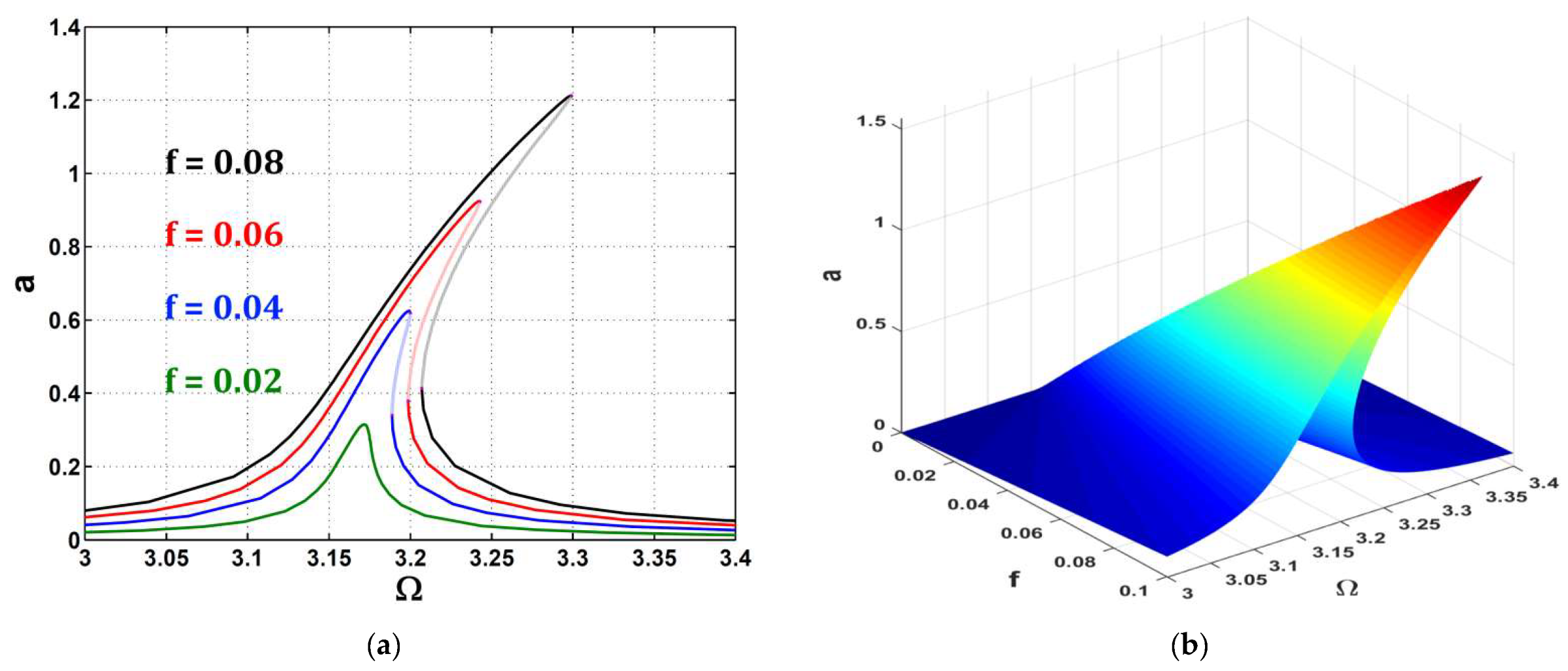
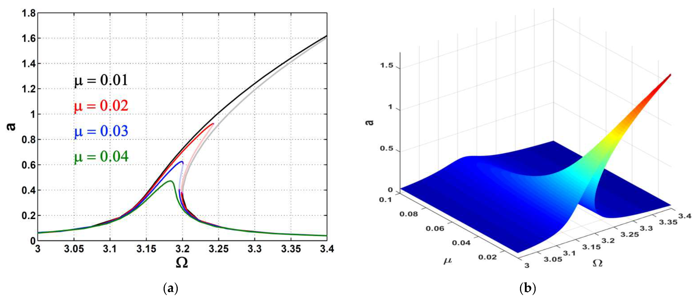
• The right-bending of the car’s vibration amplitude curve increased with the excitation force amplitude, which made the nonlinearity effect appear due to the spring’s hardening phenomenon.
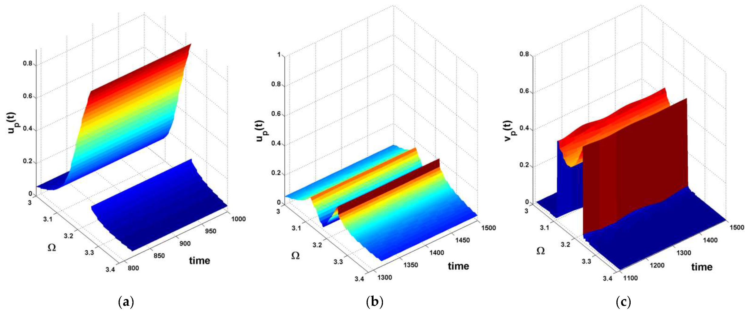
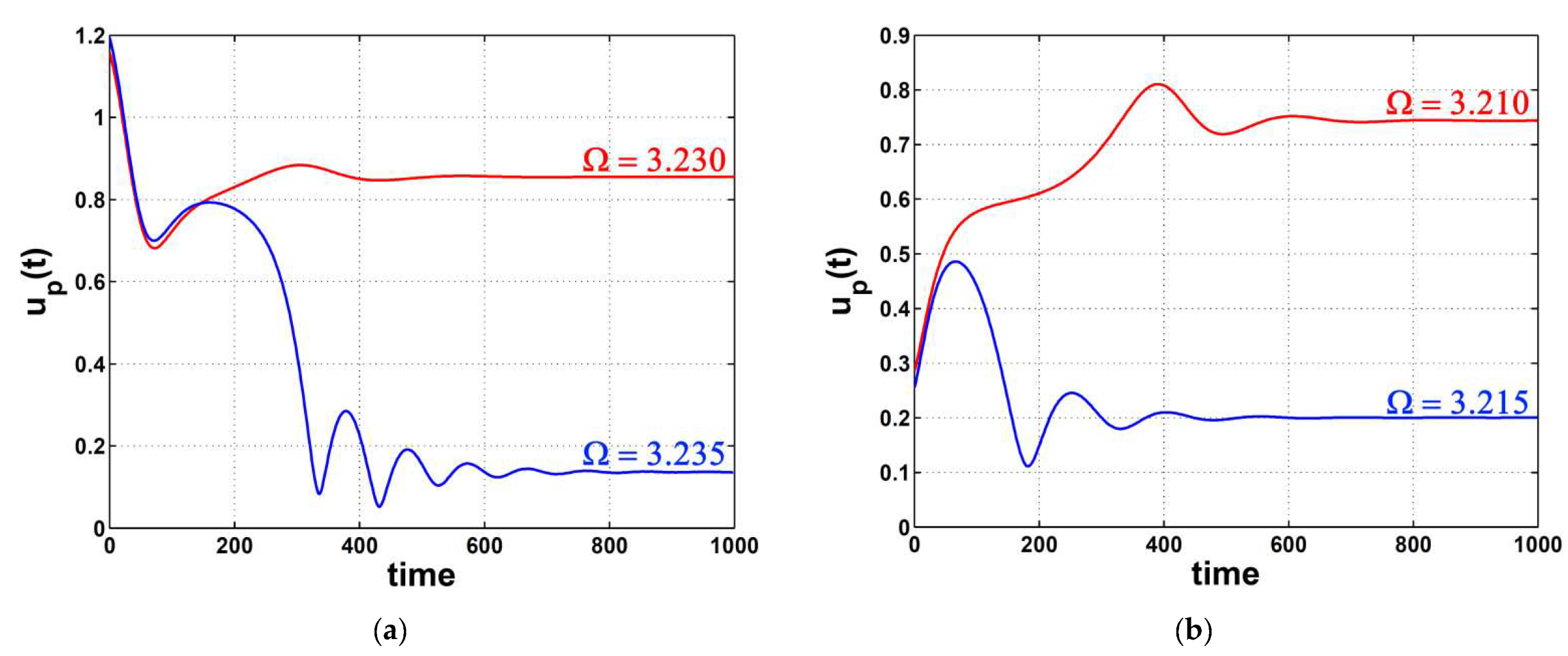
• The jump phenomena displayed high to low states, and vice versa.
• The damping parameter could suppress the maximum amplitude, in addition to eliminating the existence of saddle-node points and therefore also the jump phenomena.
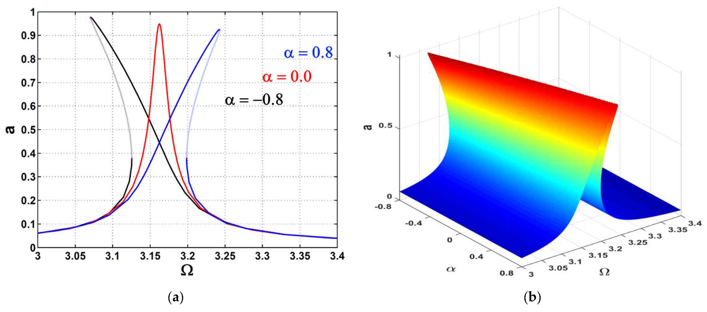
• The amplitude curve was exposed to a right-bending case (hardening phenomenon), a left-bending case (softening phenomenon), or a linear case depending on the sign of the cubic nonlinearity parameter.
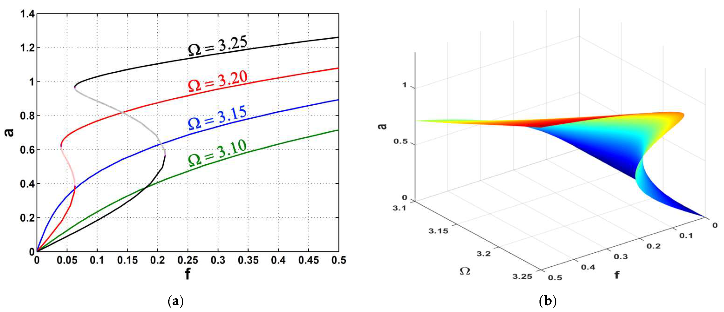
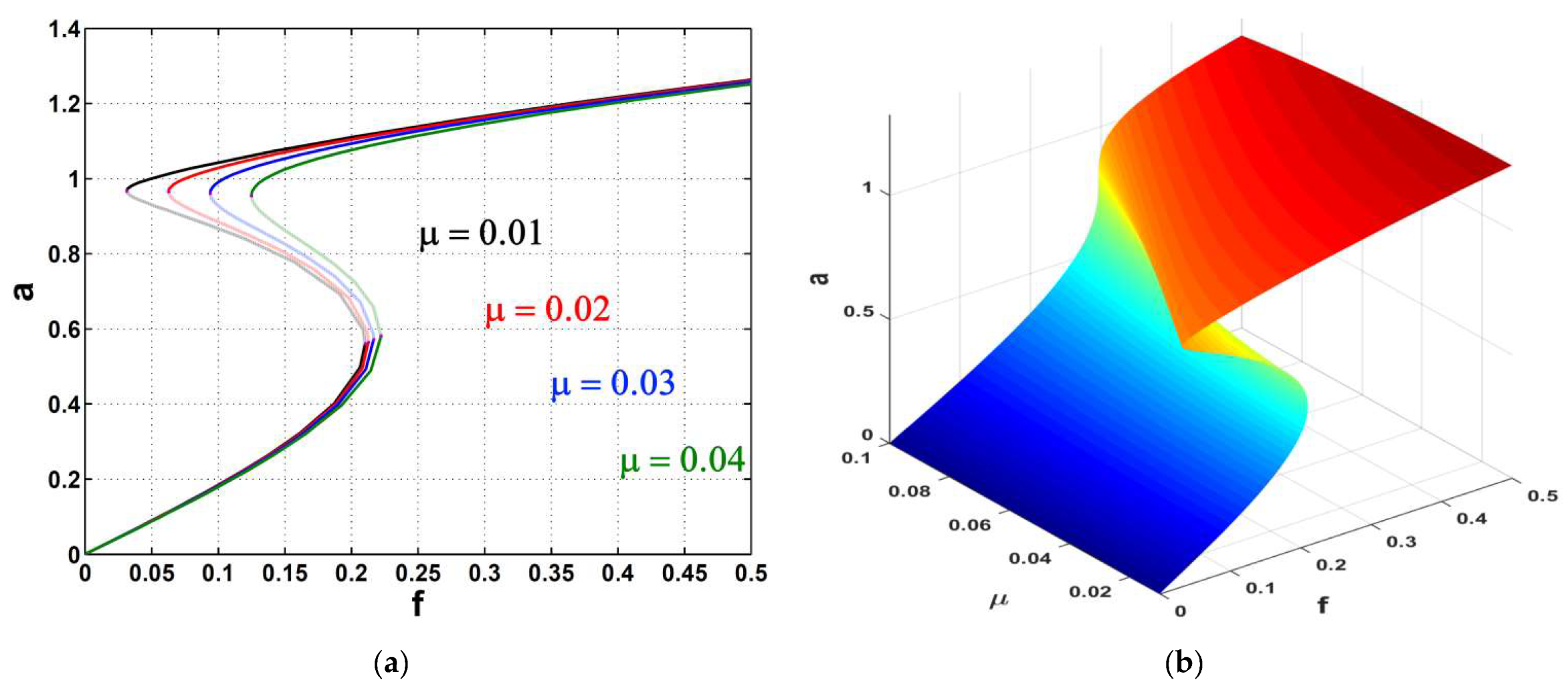
• The excitation force amplitude and the damping factor could play an important role in tightening the range of the jump phenomena on the amplitude curve.

B.

When the controller was ON:

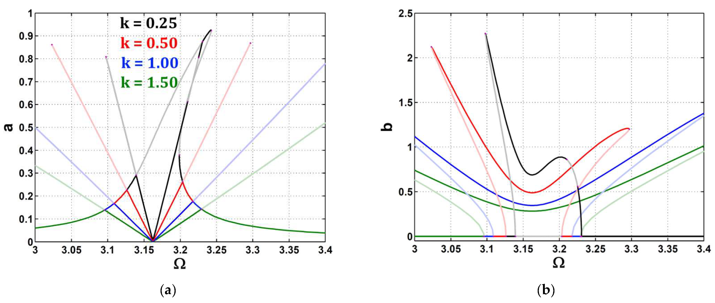
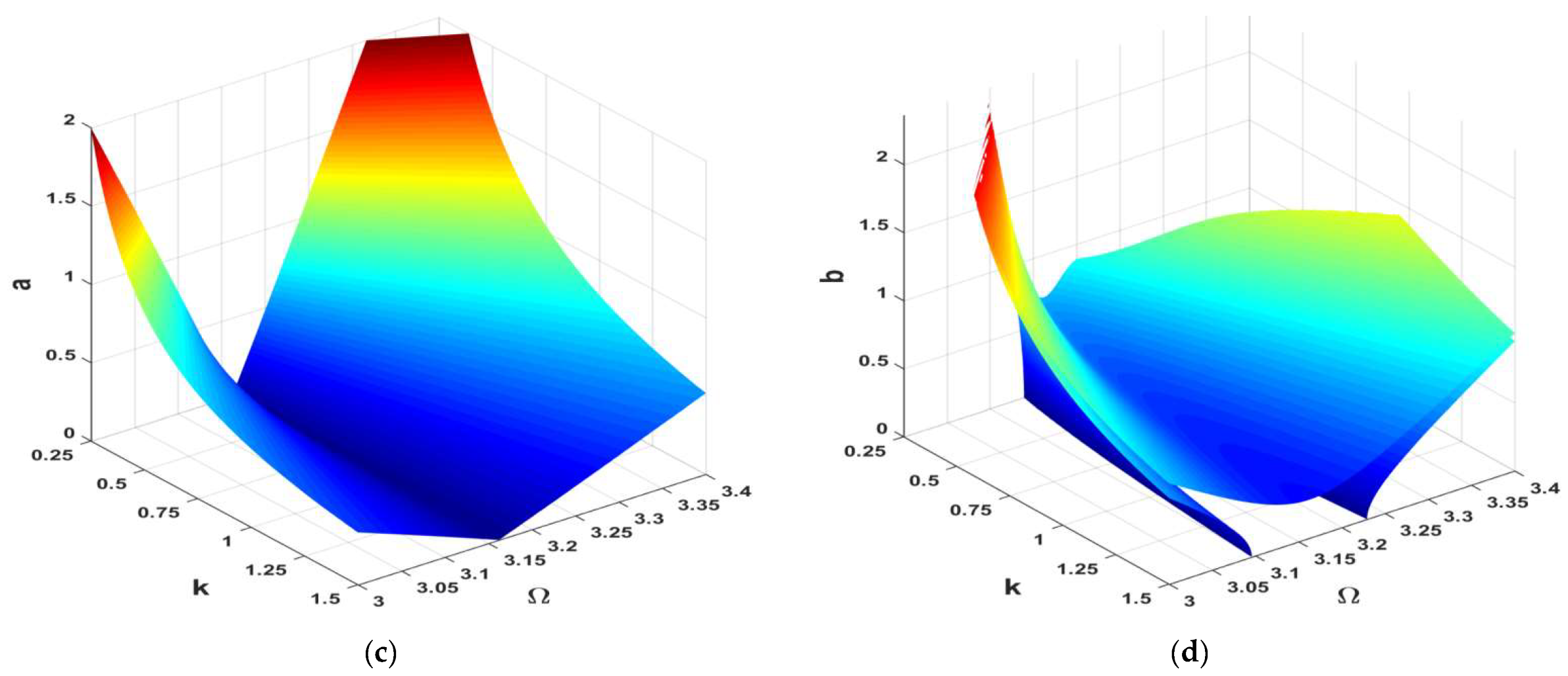
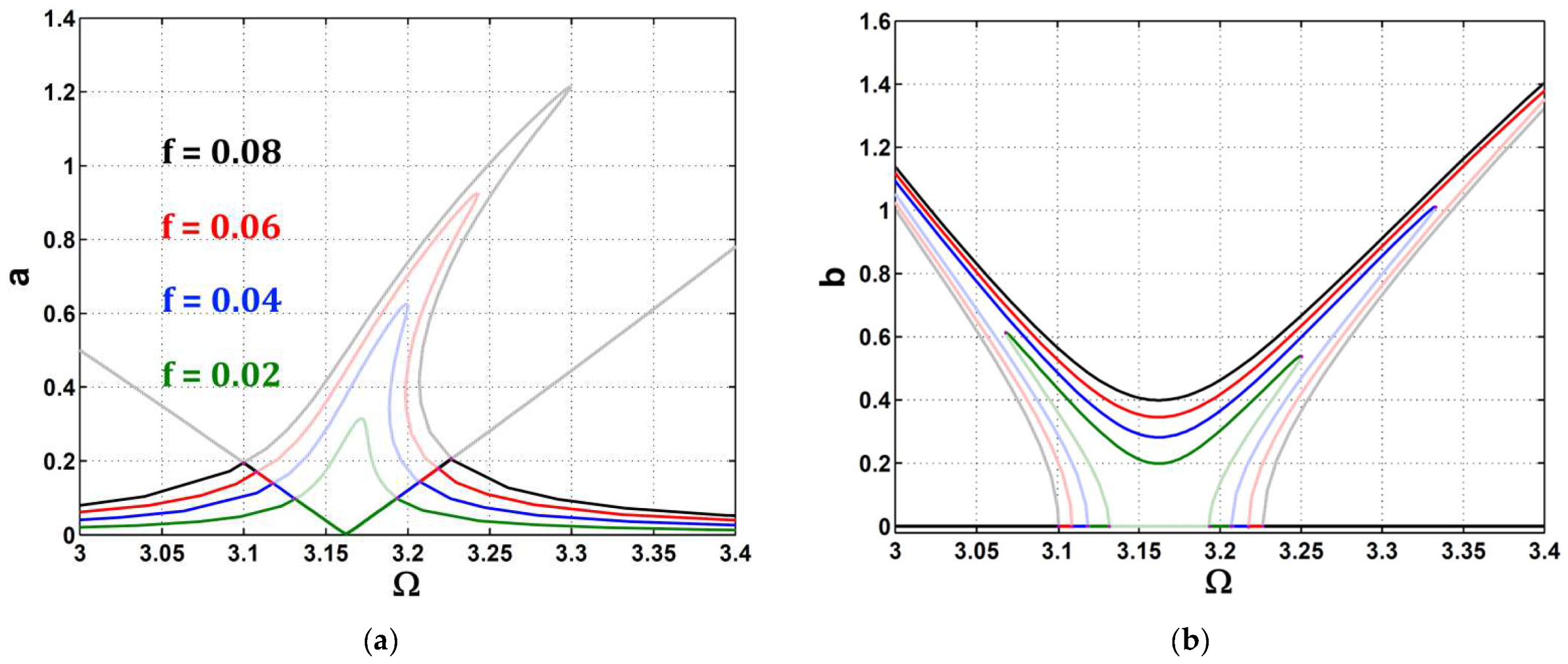
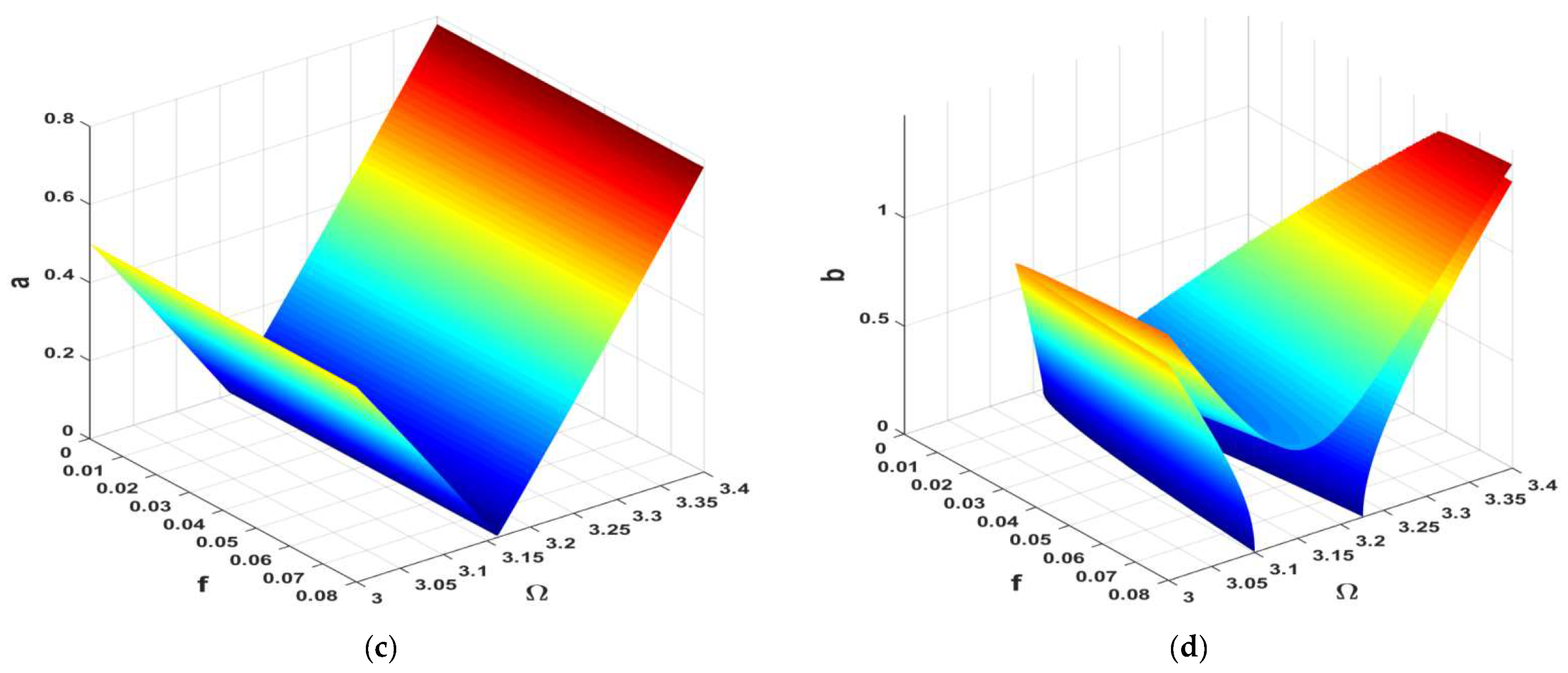
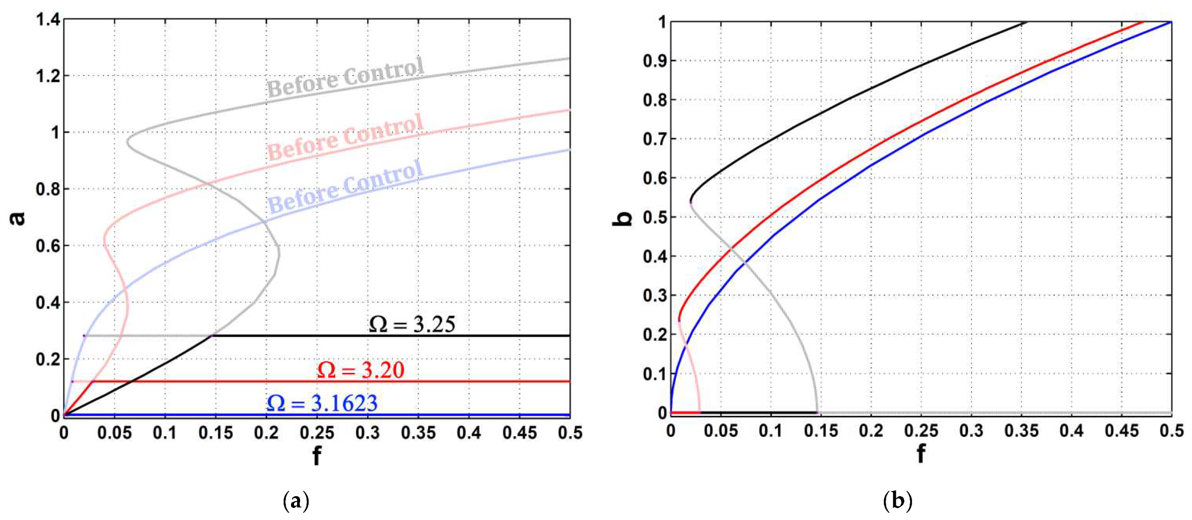
• The car’s amplitude took a new V-shaped path, departing from the previous path of higher values.
• The control and feedback gains could control the intersection band between the V-curve and the previous curve, where the bigger the gains were, the wider the V-curve became.
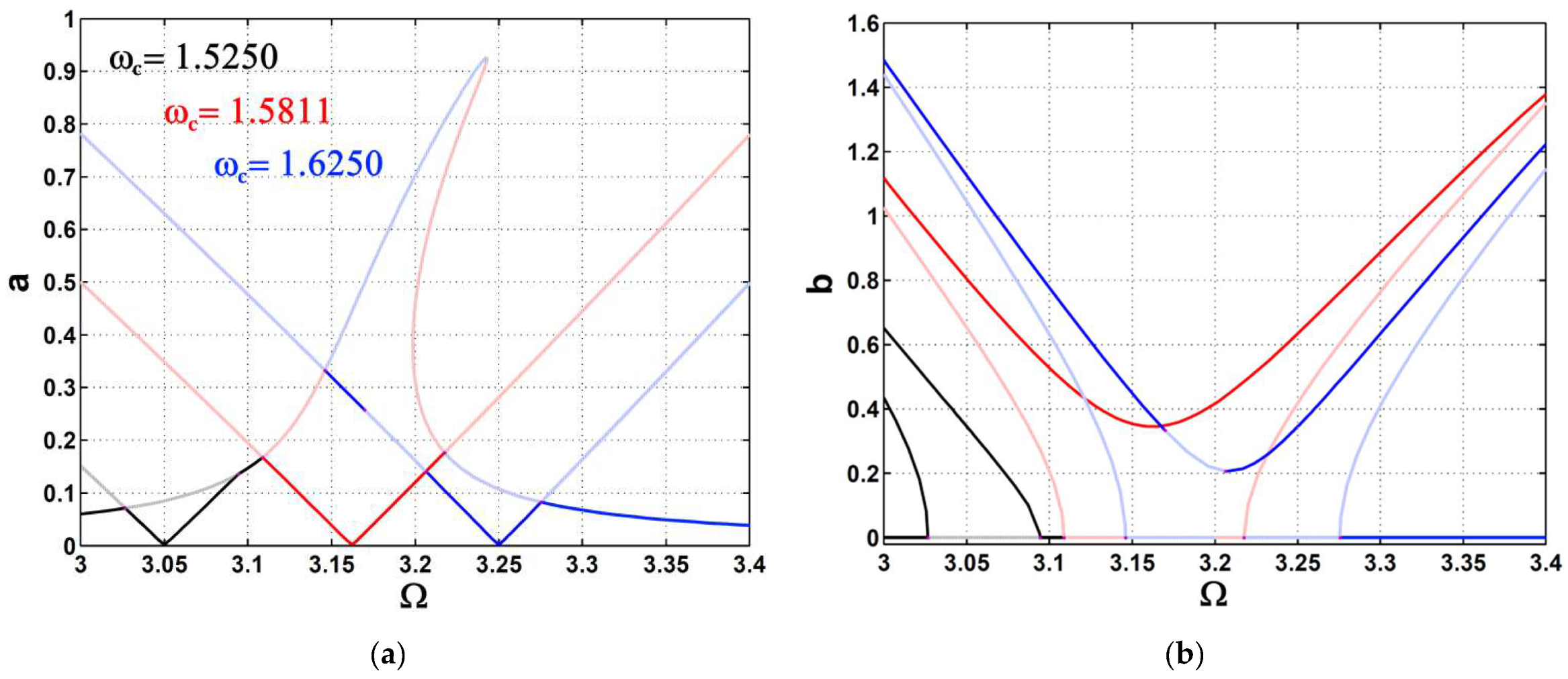
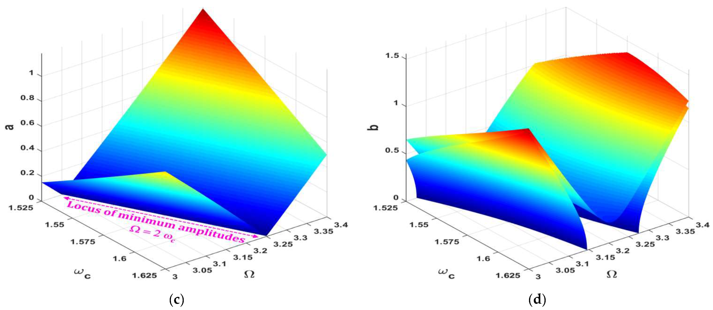
• The apex of the V-curve was at the point $\mathsf{\Omega }=\omega =2{\omega }_c$ at which the system was designed to run.
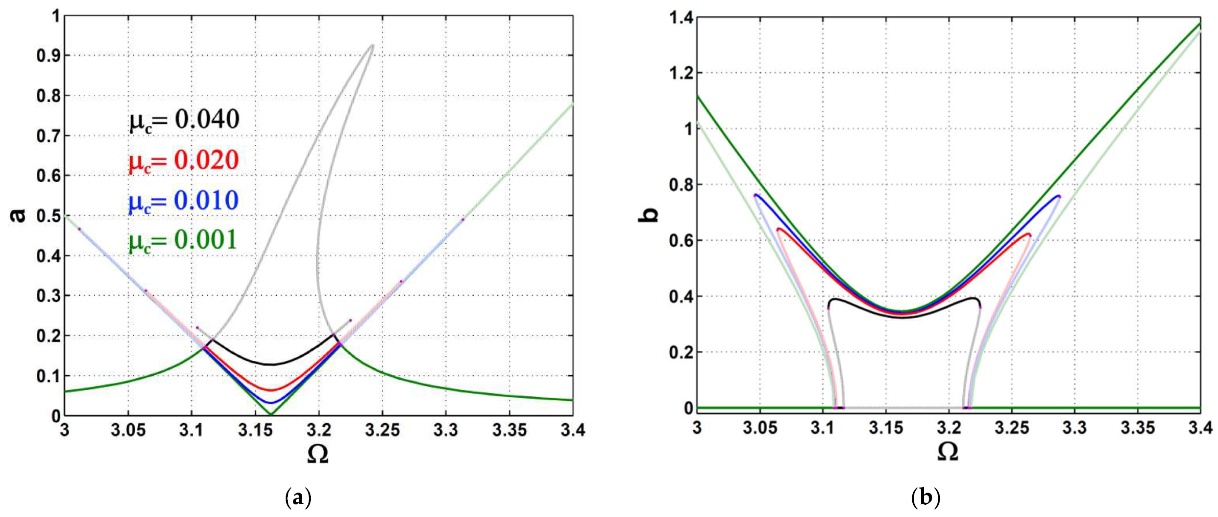
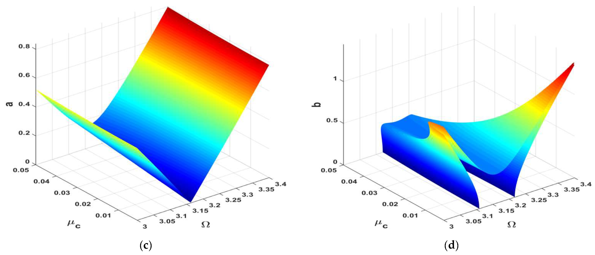
• Keeping the controller’s damping parameter at lower values took the car’s amplitude to its minimum level.
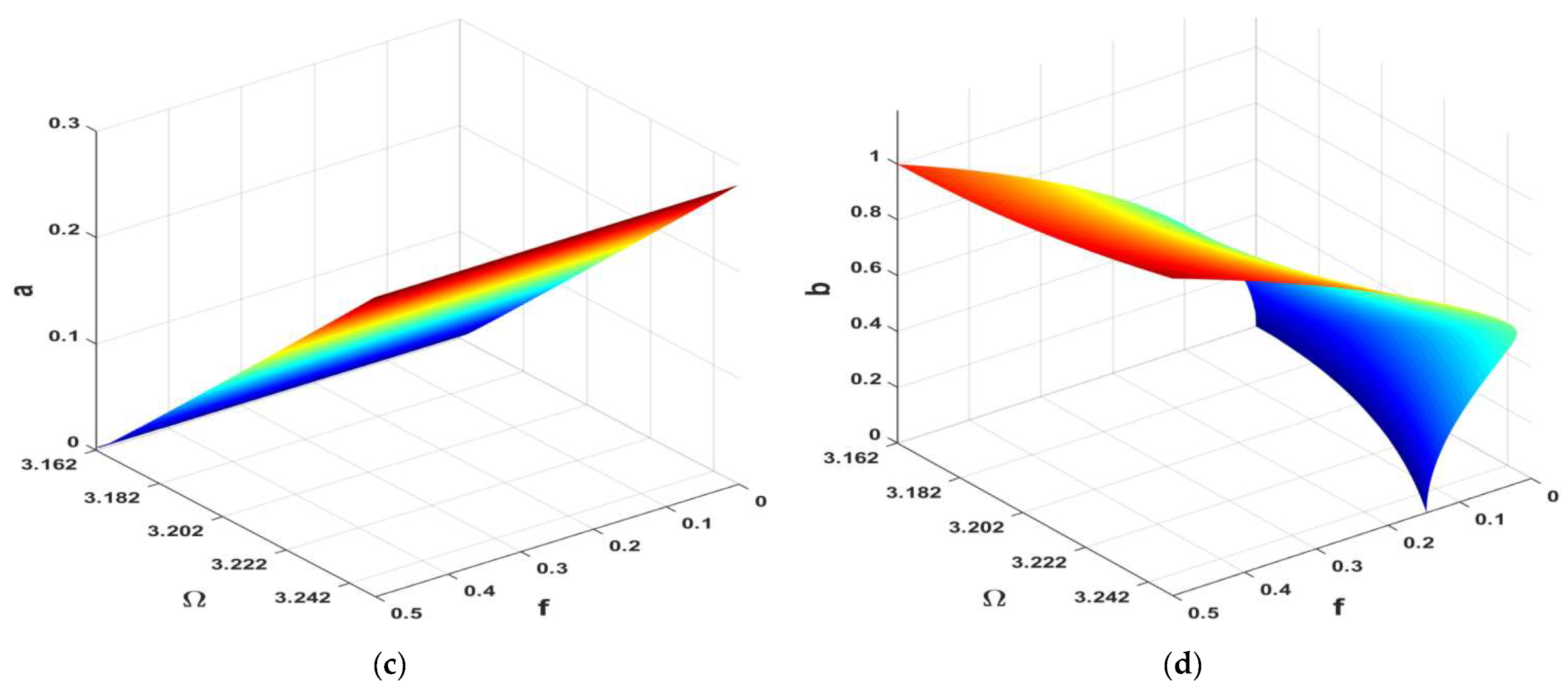
• The car’s amplitude was saturated at a specific level, keeping the V-curve unchanged even if the excitation force changed.
• The key to keeping the car’s amplitude at almost zero was to guarantee that $\mathsf{\Omega }=2{\omega }_c$ even if the excitation frequency changed.
• In case of mistuning such that $\mathsf{\Omega }\ne 2{\omega }_c$, the car’s amplitude could increase slightly with $f$ until a specific value of $\mathsf{\Omega }$ at which the amplitude could saturate independently of $f$.
• The car’s vibrations were suppressed by about $96\%$ according to the numerical simulations of the studied model.

References

1. Hamdan, M.N.; Burton, T.D. On the steady state response and stability of non-linear oscillators using harmonic balance. J. Sound Vib. 1993, 166, 255–266. [Google Scholar] [CrossRef]
2. Hassan, A. On the local stability analysis of the approximate harmonic balance solutions. Nonlinear Dyn. 1996, 10, 105–133. [Google Scholar] [CrossRef]
3. Hamdan, M.N.; Shabaneh, N.H. On the period of large amplitude free vibration of conservative autonomous oscillators with static and inertia type cubic non-linearities. J. Sound Vib. 1997, 199, 737–750. [Google Scholar] [CrossRef]
4. Maccari, A. Response of an oscillator moving along a parabola to an external excitation. Nonlinear Dyn. 2000, 23, 205–223. [Google Scholar] [CrossRef]
5. Al-Qaisia, A.A.; Hamdan, M.N. Bifurcations and chaos of an immersed cantilever beam in a fluid and carrying an intermediate mass. J. Sound Vib. 2003, 253, 859–888. [Google Scholar] [CrossRef]
6. Dunne, J.F. Subharmonic-response computation and stability analysis for a nonlinear oscillator using a split-frequency harmonic balance method. J. Comput. Nonlinear Dyn. 2006, 1, 221–229. [Google Scholar] [CrossRef]
7. Malatkar, P.; Nayfeh, A.H. Steady-State dynamics of a linear structure weakly coupled to an essentially nonlinear oscillator. Nonlinear Dyn. 2007, 47, 167–179. [Google Scholar] [CrossRef]
8. Zhang, B.; Billings, S.A.; Lang, Z.Q.; Tomlinson, G.R. A novel nonlinear approach to suppress resonant vibrations. J. Sound Vib. 2008, 317, 918–936. [Google Scholar] [CrossRef] [Green Version]
9. Carrella, A.; Brennan, M.J.; Kovacic, I.; Waters, T.P. On the force transmissibility of a vibration isolator with quasi-zero-stiffness. J. Sound Vib. 2009, 322, 707–717. [Google Scholar] [CrossRef]
10. Gatti, G.; Brennan, M.J.; Kovacic, I. On the interaction of the responses at the resonance frequencies of a nonlinear two degrees-of-freedom system. Phys. D Nonlinear Phenom. 2010, 239, 591–599. [Google Scholar] [CrossRef] [Green Version]
11. Nayfeh, A.H.; Nayfeh, N.A. Analysis of the cutting tool on a lathe. Nonlinear Dyn. 2011, 63, 395–416. [Google Scholar] [CrossRef]
12. Luo, A.C.J.; O’Connor, D. Stable and unstable periodic solutions to the Mathieu-Duffing oscillator. In Proceedings of the IEEE 4th International Conference on Nonlinear Science and Complexity, NSC, Budapest, Hungary, 6–11 August 2012; pp. 201–204. [Google Scholar]
13. Le, T.D.; Ahn, K.K. Experimental investigation of a vibration isolation system using negative stiffness structure. Int. J. Mech. Sci. 2013, 70, 99–112. [Google Scholar] [CrossRef]
14. Ji, J.C.; Zhang, N. Suppression of the primary resonance vibrations of a forced nonlinear system using a dynamic vibration absorber. J. Sound Vib. 2010, 329, 2044–2056. [Google Scholar] [CrossRef] [Green Version]
15. Ji, J.C.; Zhang, N. Suppression of super-harmonic resonance response using a linear vibration absorber. Mech. Res. Commun. 2011, 38, 411–416. [Google Scholar] [CrossRef]
16. Ji, J.C. Secondary resonances of a quadratic nonlinear oscillator following two-to-one resonant Hopf bifurcations. Nonlinear Dyn. 2014, 78, 2161–2184. [Google Scholar] [CrossRef]
17. Ji, J.C. Two families of super-harmonic resonances in a time-delayed nonlinear oscillator. J. Sound Vib. 2015, 349, 299–314. [Google Scholar] [CrossRef]
18. Kamel, M.; Kandil, A.; El-Ganaini, W.A.; Eissa, M. Active vibration control of a nonlinear magnetic levitation system via Nonlinear Saturation Controller (NSC). Nonlinear Dyn. 2014, 77, 605–619. [Google Scholar] [CrossRef]
19. Eissa, M.; Kandil, A.; El-Ganaini, W.A.; Kamel, M. Vibration suppression of a nonlinear magnetic levitation system via time delayed nonlinear saturation controller. Int. J. Non. Linear. Mech. 2015, 72, 23–41. [Google Scholar] [CrossRef]
20. Hao, Z.; Cao, Q. The isolation characteristics of an archetypal dynamical model with stable-quasi-zero-stiffness. J. Sound Vib. 2015, 340, 61–79. [Google Scholar] [CrossRef]
21. EL-Sayed, A.T.; Bauomy, H.S. Vibration suppression of subharmonic resonance response using a nonlinear vibration absorber. J. Vib. Acoust. Trans. ASME 2015, 137. [Google Scholar] [CrossRef]
22. Motallebi, A.; Irani, S.; Sazesh, S. Analysis on jump and bifurcation phenomena in the forced vibration of nonlinear cantilever beam using HBM. J. Brazilian Soc. Mech. Sci. Eng. 2016, 38, 515–524. [Google Scholar] [CrossRef]
23. Pérez-Molina, M.; Gil-Chica, J.; Fernández-Varó, E.; Pérez-Polo, M.F. Steady state, oscillations and chaotic behavior of a gas inside a cylinder with a mobile piston controlled by PI and nonlinear control. Commun. Nonlinear Sci. Numer. Simul. 2016, 36, 468–495. [Google Scholar] [CrossRef] [Green Version]
24. Zhou, S.; Song, G.; Sun, M.; Ren, Z. Nonlinear dynamic analysis of a quarter vehicle system with external periodic excitation. Int. J. Non. Linear. Mech. 2016, 84, 82–93. [Google Scholar] [CrossRef]
25. Kandil, A.; Eissa, M. Improvement of positive position feedback controller for suppressing compressor blade oscillations. Nonlinear Dyn. 2017, 90, 1727–1753. [Google Scholar] [CrossRef]
26. Kandil, A. Study of Hopf curves in the time delayed active control of a 2DOF nonlinear dynamical system. SN Appl. Sci. 2020, 2, 1924. [Google Scholar] [CrossRef]
27. Silveira, M.; Wahi, P.; Fernandes, J.C.M. Effects of asymmetrical damping on a 2 DOF quarter-car model under harmonic excitation. Commun. Nonlinear Sci. Numer. Simul. 2017, 43, 14–24. [Google Scholar] [CrossRef] [Green Version]
28. Kandil, A.; El-Gohary, H.A. Suppressing the nonlinear vibrations of a compressor blade via a nonlinear saturation controller. JVC/J. Vib. Control. 2018, 24, 1488–1504. [Google Scholar] [CrossRef]
29. Hamed, Y.S.; Kandil, A. Influence of time delay on controlling the non-linear oscillations of a rotating blade. Symmetry 2021, 13, 85. [Google Scholar] [CrossRef]
30. Zhou, S.; Song, G.; Li, Y.; Huang, Z.; Ren, Z. Dynamic and steady analysis of a 2-DOF vehicle system by modified incremental harmonic balance method. Nonlinear Dyn. 2019, 98, 75–94. [Google Scholar] [CrossRef]
31. Kandil, A.; Hamed, Y.S. Tuned Positive Position Feedback Control of an Active Magnetic Bearings System with 16-Poles and Constant Stiffness. IEEE Access 2021, 9, 73857–73872. [Google Scholar] [CrossRef]
32. Kandil, A.; Hamed, Y.S.; Alsharif, A.M. Rotor Active Magnetic Bearings System Control via a Tuned Nonlinear Saturation Oscillator. IEEE Access 2021, 9, 133694–133709. [Google Scholar] [CrossRef]
33. Uemori, M.; Yabuno, H.; Ymamamoto, Y.; Matsumoto, S. Highly sensitive measurements of perturbations in stiffness of a resonator by virtual coupling with a virtual resonator. Nonlinear Dyn. 2021, 107, 1755–1764. [Google Scholar] [CrossRef]
34. Kandil, A.; Hamed, Y.S.; Alsharif, A.M.; Awrejcewicz, J. 2D and 3D visualizations of the mass-damper-spring model dynamics controlled by a servo-controlled linear actuator. IEEE Access 2021, 9, 153012–153026. [Google Scholar] [CrossRef]
35. Nayfeh, A.H.; Mook, D.T. Nonlinear Oscillations; Wiley: New York, NY, USA, 1995. [Google Scholar]
36. Krack, M.; Gross, J. Harmonic Balance for Nonlinear Vibration Problems; Springer Nature: Cham, Switzerland, 2019. [Google Scholar]
37. Nayfeh, A.H.; Balachandran, B. Applied Nonlinear Dynamics; Wiley: New York, NY, USA, 1995. [Google Scholar]
Figure 1. A harmonically-excited and controlled car of mass m .
Symmetry 14 01247 g001
Figure 2. Implementation of the control unit.
Symmetry 14 01247 g002
Figure 3. Diagrammatic description of: (a) the multiplier (MUL) unit, and (b) the squarer (SQR) unit.
Symmetry 14 01247 g003
Figure 4. The car’s vibration amplitude a responded to the excitation frequency Ω at excitation forces f = { 0.02 , 0.04 , 0.06 , 0.08 } when NSC was OFF: (a) a as a function of Ω , (b) a as a function of Ω and f .
Symmetry 14 01247 g004
Figure 5. The car’s vibration amplitude a responded to the excitation frequency Ω at damping factors μ = { 0.01 , 0.02 , 0.03 , 0.04 } with NSC turned OFF: (a) a as a function of Ω , (b) a as a function of Ω and μ .
Symmetry 14 01247 g005
Figure 6. The car’s vibration amplitude a respondedto the excitation frequency Ω at cubic stiffness factors α = { 0.8 , 0.0 , 0.8 } with NSC turned OFF: (a) a as a function of Ω , (b) a as a function of Ω and α
Symmetry 14 01247 g006
Figure 7. The car’s vibration amplitude a responded to the excitation force amplitude f at excitation frequencies Ω = { 3.10 , 3.15 , 3.20 , 3.25 } with NSC switched OFF: (a) a as a function of f , (b) a as a function of f and Ω .
Symmetry 14 01247 g007
Figure 8. The car’s vibration amplitude a responded to the excitation force amplitude f at damping factors μ = { 0.01 , 0.02 , 0.03 , 0.04 } when NSC was OFF: (a) a as a function of f , (b) a as a function of f and μ .
Symmetry 14 01247 g008
Figure 9. (a,c) The car’s vibration amplitude a , and (b,d) the controller’s amplitude b responded to the excitation frequency Ω at control gains k = { 0.25 , 0.50 , 1.00 , 1.50 } when NSC was ON.
Symmetry 14 01247 g009aSymmetry 14 01247 g009b
Figure 10. (a,c) The car’s vibration amplitude a , and (b,d) the controller’s amplitude b responded to the excitation frequency Ω at controller damping factors μ c = { 0.001 , 0.01 , 0.02 , 0.04 } when NSC was ON.
Symmetry 14 01247 g010aSymmetry 14 01247 g010b
Figure 11. (a,c) The car’s vibration amplitude a , and (b,d) the controller’s amplitude b responded to the excitation frequency Ω at excitation forces f = { 0.02 , 0.04 , 0.06 , 0.08 } when NSC was ON.
Symmetry 14 01247 g011aSymmetry 14 01247 g011b
Figure 12. (a,c) The car’s vibration amplitude a , and (b,d) the controller’s amplitude b responded to the excitation frequency Ω at controller natural frequencies ω c = { 1.5250 , 1.5811 , 1.6250 } when NSC was ON.
Symmetry 14 01247 g012aSymmetry 14 01247 g012b
Figure 13. (a,c) The car’s vibration amplitude a , and (b,d) the controller’s amplitude b responded to the excitation force amplitude f at excitation frequencies Ω = { 3.1623 , 3.20 , 3.25 } when NSC was ON.
Symmetry 14 01247 g013aSymmetry 14 01247 g013b
Figure 14. Steady-state 3D simulations of the time-frequency response for the car’s vibration peaks u p t and the controller’s vibration peaks v p t when: (a) NSC was OFF, (b,c) NSC was ON.
Symmetry 14 01247 g014
Figure 15. Simulations of the time response for the car’s vibration peaks u p t when NSC was OFF and: (a) sweeping Ω up where the car’s vibration jumps from HIGH to LOW, (b) sweeping Ω down where the car’s vibration jumped from LOW to HIGH
Symmetry 14 01247 g015
Figure 16. Simulations of the time response for: (a) the car’s vibration peaks u p t , and (b) the controller’s vibration peaks v p t with NSC turned OFF (red) or ON (blue) at f = 0.06 and Ω = ω = 3.1623 .
Symmetry 14 01247 g016
Publisher’s Note: MDPI stays neutral with regard to jurisdictional claims in published maps and institutional affiliations.