Article

CLHF-Net: A Channel-Level Hierarchical Feature Fusion Network for Remote Sensing Image Change Detection

College of Information Science and Engineering, Xinjiang University, Urumqi 830017, China
*
Author to whom correspondence should be addressed.
Symmetry 2022, 14(6), 1138; https://doi.org/10.3390/sym14061138
Submission received: 5 May 2022 / Revised: 24 May 2022 / Accepted: 26 May 2022 / Published: 1 June 2022

Abstract

:
Remote sensing (RS) image change detection (CD) is the procedure of detecting the change regions that occur in the same area in different time periods. A lot of research has extracted deep features and fused multi-scale features by convolutional neural networks and attention mechanisms to achieve better CD performance, but these methods do not result in well-fused feature pairs of the same scale and features of different layers. To solve this problem, a novel CD network with symmetric structure called the channel-level hierarchical feature fusion network (CLHF-Net) is proposed. First, a channel-split feature fusion module (CSFM) with symmetric structure is proposed, which consists of three branches. The CSFM integrates feature information of the same scale feature pairs more adequately and effectively solves the problem of insufficient communication between feature pairs. Second, an interaction guidance fusion module (IGFM) is designed to fuse the feature information of different layers more effectively. IGFM introduces the detailed information from shallow features into deep features and deep semantic information into shallow features, and the fused features have more complete feature information of change regions and clearer edge information. Compared with other methods, CLHF-Net improves the F1 scores by 1.03%, 2.50%, and 3.03% on the three publicly available benchmark datasets: season-varying, WHU-CD, and LEVIR-CD datasets, respectively. Experimental results show that the performance of the proposed CLHF-Net is better than other comparative methods.

1. Introduction

Change detection (CD) is the detection of changes that occur in the same area at different times [1], and it has important practical applications for the development of satellite technology. CD plays a crucial role in urban resource management, land-use planning, disaster assessment, and analysis of military or civilian activities [2,3,4]. In recent years, with the rapid development of various computer vision techniques [5,6,7], CD is becoming an active research topic [8,9,10].
CD methods usually need to achieve two objectives: reducing or eliminating the interference of semantic noise and accurately detecting the localized change regions. In recent years, convolutional neural networks (CNNs), especially fully convolutional neural networks (FCNs) [11], have successfully broken through the bottlenecks of traditional manual feature methods and driving CD tasks, achieving significant improvements in [11,12,13,14,15]. Since CD tasks have dual/multiple inputs, convolutional networks for image CD can be divided into pre-fusion networks and post-fusion networks according to the input fusion strategy [10]. The pre-fusion methods can capture more information about the foreground region, corresponding to the deeper features of the network, while post-fusion methods can express more detailed information, corresponding to the shallow features of the network [8]. However, most of the existing methods based on pre-fusion or post-fusion strategies address one of these aspects. This may lead to various inaccurate detection phenomena.
To solve the feature fusion problem of bi-temporal images and to achieve a more effective feature fusion method for bi-temporal images, a CD method based on a channel-level hierarchical feature fusion network (CLHF-Net) is proposed in this paper. The proposed method better focuses on the channel communication between two bi-temporal feature maps at the same scale and tries to explore the importance of different channels of a feature map in the feature representation. In the decoding stage, the effective fusion of multi-scale features is achieved by using progressive fusion to further improve the detection accuracy.
In summary, the main contributions of this article are as follows:
  • We propose a novel CD network with symmetric structure, called the channel-level hierarchical feature fusion network (CLHF-Net). It aims to solve the problems of insufficient communication between bi-temporal feature pairs and inadequate feature fusion in channel groups.
  • A channel-split feature fusion module (CSFM) with symmetric structure is proposed, which consists of three parts, namely the channel splitting branch (CSB), interaction fusion unit (IFU), and feature aggregation branch (FAB). The CSB splits the feature map into multiple channel-group features. The IFU is designed to enable effective communication and adequate fusion of channel multi-group feature pairs. The FAB integrates the input feature pairs and the fused features, resulting in a higher quality change feature map.
  • To fuse the semantic features of different levels more effectively, an interaction guidance fusion module (IGFM) is proposed. First, the IGFM introduces high-level semantic information into low-level features, which can eliminate the redundant semantic information in shallow features. The low-level detailed feature information is introduced into the high-level features, which can compensate the detailed semantic information in the deep features. Then, convolution and attention operations are implemented to further fuse the two updated features.
The next parts of this paper are laid out as follows: Section 2 reviews the literature on CD methods. Section 3 is the detailed description part of the proposed method. Section 4 is a series of experimental parts to verify the performance of the proposed method. Section 5 is the ablation study part that further verifies the effectiveness of each innovative module of the proposed method. Section 6 concludes the work of this paper.

2. Related Work

The existing CD methods can be roughly classified into traditional methods [16] and deep learning (DL)-based methods [4], and each will be briefly introduced in the following sections.

2.1. Traditional Methods

According to the different analysis units, the traditional CD methods can be divided into pixel-based CD methods and object-based CD methods [16,17]. In the early stage, methods such as regression analysis, image ratio, and image difference [18,19,20] were widely used, but there were some differences between their detection results and the ground truth, and there were cases of missed and false detections. To improve the utilization of spectral information from RS images, CD methods based on image transformation have emerged one after another, such as the independent component analysis (ICA) method [21] and the multivariate alteration detection (MAD) method [22]. In 2007, Bovolo and Bruzzone [23] introduced the concept of multi-classification CD and proposed the change vector analysis (CVA) method based on a polar coordinate domain for multi-spectral images. However, the stability of the CVA algorithm cannot be guaranteed because the performance is limited by the quality of the spectral bands. Therefore, Bovolo et al. [24] proposed an improved version of compressed CVA ( C 2 VA ) in 2012, which eliminates the blindness of spectral band selection and reduces the loss of spectral band information, further improving the performance. Lui et al. [25,26] proposed the hierarchical spectral CVA (HSCVA) method and the sequential spectral CVA ( S 2 CVA ) method in 2015. Combining the extremely large number of spectral bands of hyperspectral images, the variations are continuously subdivided down. They successfully applied it to the hyperspectral RS image CD task. In 2017, Zanetti et al. [27] proposed a theoretical framework for a representation of the statistical distribution of difference maps as a composite model and extended the traditional CVA to multi-class situations. In recent years, Ghaderpour and Vujadinovic [28] have innovatively proposed the jumps upon spectrum and trend (JUST) CD method. JUST identifies potential jumps by considering the appropriate weights associated with the time series and can address the instability and uneven sampling intervals of time series RS data and the challenges posed by atmospheric effects in the RS CD process. JUST can directly be applied to detecting changes within RS satellite data that may have gaps or missing values without any need for interpolation [29]. In 2021, Masiliūnas et al. [30] proposed an unsupervised time series CD algorithm to aid the upscaling of BFAST for global land cover CD. However, pixel-based CD only uses the feature information of individual pixels, ignoring the spatial and spectral information of neighboring pixels, which is prone to noise effects and incomplete representation of the change region.
The object-based CD method integrates the spectral information of image elements and the spatial information of image element neighbors, which helps to reduce the false alarm rate and missed alarm rate in the difference map. Su et al. [31] presented a CD algorithm that combines object-level and pixel-level representations to extract change regions containing artificial objects. Wang et al. [32] proposed a new unsupervised CD technique for color satellite multi-temporal images. A computationally simple method for singular value decomposition (SVD) is adopted to perform principal component analysis (PCA) on the pure quaternion image. Benedek et al. [33] introduced a conditional mixed Markov model, which compares the segmented images for differences. Inglada et al. [34] proposed a new similarity for automatic CD of a multi-temporal synthetic aperture radar images metric. The method uses Kullback–Leibler divergence to measure local change information. Wang et al. [35] presented a CD method based on a triple Markov field (TMF) model. The adaptive weight parameter from the previous energy is introduced to cope with the detection trade-off problem to obtain an automatic estimation of parameters with low complexity. Wang et al. [36] proposed a robust objective-level CD method by combining multi-feature extraction with integration learning. In 2018, Zhang et al. [37] optimized the performance of CD by introducing the idea of multi-scale uncertainty analysis and using support vector machine (SVM) classifiers to iteratively analyze uncertain change regions. Based on this, Tan et al. [38] further improved the CD by using multiple classifiers involved in uncertain region change analysis and fusing these classification results for decision making. While the object-based CD method integrates the spatial and spectral information from the original image, it is sensitive to both alignment errors and object shadows, which may limit the detection accuracy.

2.2. Deep-Learning-Based Methods

With the success of DL techniques in computer vision (CV), DL-based CD methods are gradually becoming a research trend. From the fusion stage of bi-temporal RS images, DL-based CD methods can be roughly divided into two types: pre-fusion CD and post-fusion CD [39].
The input to a network using a pre-fusion strategy is the result of concatenation of image pairs or a difference map of image pairs. The late fusion CD method refers to first inputting two bi-temporal images into the network separately, obtaining the features of the two images separately, and then fusing the two sets of features obtained. For example, Daudt et al. [10] proposed three models, namely fully convolutional early fusion (FC-EF), fully convolutional Siamese-concatenation (FC-Siam-Conc), and fully convolutional Siamese-difference (FC-Siam-Diff). The FC-EF structure concatenates two images and takes the concatenated images as the input to the network. The Siamese structure takes two images as input to the network, respectively, where the parameter weights of the network are shared, and then uses a convolutional layer to merge the two outputs. The deeply supervised image fusion network (DSIFN) designed by Zhang et al. [8] also employs a late fusion strategy. The DSIFN fuses the deep features extracted by the Siamese network on a dual-stream architecture and feeds them into the difference inference network for CD. To overcome the heterogeneity problem, they introduce a convolutional block attention module (CBAM) in the decoding process [40]. To explore the effectiveness of multi-level feature fusion, Lei et al. [41] used a concatenated CNN to extract features. Fang et al. [42] presented a densely connected Siamese network (SNUNet-CD) based on the Siamese network and UNet++, in which the ensemble channel attention module (ECAM) was applied to aggregate and refine features at multiple semantic levels. As the research progressed, it was noticed that neither early fusion nor late fusion strategies could make the network achieve the best performance. Therefore, Wang et al. [43] proposed an attention mechanism-based deep supervision network (ADS-Net), which uses a mid-layer fusion approach for feature fusion.
In addition, cross-domain research often yields unexpected results. Researchers have tried to introduce new results from other fields into the CD task. For example, Zhang et al. [44] presented a hierarchical dynamic fusion network (HDFNet), which introduces a dynamic convolution module in the decoding stage to enhance feature fusion and further refine the feature representation. Similarly, Hou et al. [45] designed a CD network with three branches. To utilize the temporal information embedded in the images, a dynamic inception module was designed in this network. As the research progresses, the design of the network structure shows the fantastic conceptions of the researchers. For example, Zheng et al. [46] presented a U-Net-based cross-layer convolutional neural network (CLNet), which designed cross-layer blocks (CLBs) to fuse contextual semantic information from different layers. To better extract to deep and shallow features in images, Yang et al. [47] designed a new asymmetric Siamese network that achieves better CD performance. Many works such as these give us inspiration and thoughts to explore more effective CD methods.
In recent years, the introduction of attentional mechanisms has made a significant impact on the performance of CD tasks. Chen et al. [48] proposed a dual-attention fully convolutional Siamese network (DASNet) to extract features of image pairs, and the resulting features were used to modify the contrast loss and thus improve the performance of the model. To generate more discriminative features, Chen et al. [49] proposed a spatial–temporal attention neural network (STANet). The STANet uses Siamese FCNs to extract diachronic images and proposes two attention modules. Song et al. [50] proposed an attention-based end-to-end CD network called AGCDetNet, which uses spatial attention to enhance the feature representation of change information and channel attention to improve accuracy. The number of parameters of the attention mechanism is very small and the improvement in network performance is significant, and this advantage has led to a preference for using attention to help improve the performance of the network.

3. Proposed Method

In this section, we will first introduce the overall structure and workflow of CLHF-Net. Then, the detailed structure of each innovation module is presented.

3.1. The Proposed CLHF-Net Network

With the progress of RS satellite technology, the RS images obtained by people contain richer and more complex feature information, which increases the difficulty of image feature extraction. As with most binary CD methods, the network input consists of two bi-temporal images, denoted as T1 and T2, with dimensions C × H × W , where C is the number of channels, and eventually produces a change map with a channel number of 1, whose width and height are the same as the input image. For each pixel of the change map, 1 represents change and 0 represents no change. In this paper, a channel-level hierarchical feature fusion network (CLHF-Net) with symmetric structure is proposed to deal with the CD task. The overall architecture of CLHF-Net is shown in Figure 1, and the whole network architecture adopts an encoder–decoder structure. In addition, inspired by a previous study [51,52], a channel-split feature fusion module (CSFM) is proposed to adequately fuse the bi-temporal feature maps. In the decoding phase, an interaction guidance fusion module (IGFM) is proposed to fuse high- and low-level features.
As with many previous works [53,54,55], we use two ResNet18 [56] with shared weights as the backbone of our network, which extracts features from the original image pairs, where RB1-4 denotes the residual convolution block of the ResNet18 backbone layer. Structurally, the backbone network is symmetrical. The multi-level feature pairs extracted by the backbone network are forwarded to CSFM separately, and then the fused features updated by CSFM are further processed. As shown in Figure 1, a feature pyramid-like structure is used to fuse the CSFM updated features progressively from higher to lower levels. In this step, the proposed IGFM uses an interactive fusion strategy to make the features at the higher and lower levels perform sufficient communication. It can be noticed that throughout the decoding process, there is a Convs-N (N denotes 1, 2, 3, 4) branch, and each Convs consists of two convolution blocks (Conv+BN+ReLU). Its main role is to change the number of channels of the feature map at each stage and to use the up-sampling operation so that the size of the feature map is the same as the original image. Finally, the four sets of Convs output feature maps are sent to a pixel classifier to produce the final prediction maps.

3.2. Channel-Split Feature Fusion Module

The proposed CSFM with symmetric structure is shown in Figure 2, which consists of a channel splitting branch (CSB), an interaction fusion unit (IFU), and a feature aggregation branch (FAB). The CSB splits the input features with the number of channels C into multi-group features with the number of channels c. According to a series of experimental results, the network performance is best when c is 16. This work adopts the channel splitting strategy for the following considerations: (1) Directly connecting two feature maps for feature fusion will weaken the between channel group feature pairs communication interaction. (2) Different channel group features have different importance for the representation of semantic information. It is meaningful to study which is more effective: direct fusion of two input feature maps or separate weighted fusion of channel group feature pairs.
Next, multi-group feature pairs of bi-temporal features output from the CSB are fed to the IFU, respectively. The IFU is used to capture local and global contextual semantic information. As can be seen from Figure 2, the IFU mainly consists of channel attention (CA) and spatial attention (SA) [40], which are defined as Equations (1) and (2):
C A ( F ) = σ ( M L P ( A v g ( F ) ) + M L P ( M a x ( F ) ) )
S A ( F ) = σ ( f 3 × 3 [ A v g ( F ) , M a x ( F ) ] )
where MLP denotes the multi-layer perceptron module with two 1 × 1 convolutional layers. Avg and Max represent the average pooling layer and the max pooling layer, respectively. f 3 × 3 represents the 3 × 3 convolutional layer. σ represents the sigmoid function. [.,.] denotes the concatenation operation. We found experimentally that the use of channel attention-multiplication interaction can filter out some distracting factors in non-changing regions, improve the feature fusion effect, and enhance the feature representation of changing regions.
Specifically, first, in IFU, we apply CA operations to the two input features separately. The CA maps A C a 1 c × 1 × 1 and A C b 1 c × 1 × 1 are obtained, respectively. Next, we adopt a deep interaction fusion strategy to enhance the feature fusion effect. The specific implementation is shown in Equations (3) and (4):
f a , b 1 , c = C A ( f a 1 ) f b 1 + f a 1
f b , a 1 , c = C A ( f b 1 ) f a 1 + f b 1
where is the channel-wise multiplication, and is the element-wise summation. As can be seen from Equation (3) and (4), we also add the original input features to the features obtained after interaction fusion to retain some important information of the original and enhance the feature representation. Then, we apply SA operations to the two interaction fused features f a , b 1 , c c × H 1 × W 1 and f b , a 1 , c c × H 1 × W 1 , respectively. The SA maps A S a 1 1 × H 1 × W 1 and A S b 1 1 × H 1 × W 1 are obtained, respectively. We   apply   the   product   operation   on   f a , b 1 , c and f b , a 1 , c   with   their   respective   S A   maps . The following equations are shown:
  f a , b 1 , s = S A ( f a , b 1 , c ) f a , b 1 , c
f b , a 1 , s = S A ( f b , a 1 , c )   f b , a 1 , c
where is the element-wise multiplication. The SA operation further filters out the background factors and highlights the representation of the change regions. Finally, the element-wise summation operation is performed on f a , b 1 , s and f b , a 1 , s to obtain the output features of IFU:
f a b 1 = f a , b 1 , s f b , a 1 , s
where is the element-wise summation. Next, the feature aggregation branch performs two main tasks. First, we perform a concatenation operation on the output feature map of IFU to obtain a feature map F ab C 1 × H 1 × W 1 with the same size as the input features. Second, we concatenate F ab with the two inputs F a C 1 × H 1 × W 1 and F b C 1 × H 1 × W 1 of CSFM, followed by a 3 × 3 convolution layer to obtain the final output features of CSFM.

3.3. Interaction Guidance Fusion Module

The interaction guidance fusion module (IGFM) introduces high-level semantic information into the low-level features. With the guidance of the high-level features, the redundant spatial information in the low-level features can be eliminated. Different from the low-level features, some detailed semantic information (such as boundary features) may be lost in the high-level features due to the deepening of the network layers. The detailed semantic information of low-level is introduced into the high-level features to make up for the lack of detailed features in the high-level features. The structure of the IGFM is shown in Figure 3.
Specifically, in IGFM, first, a bilinear up-sampling operation is applied to the high-level features F h C 1 × H 1 × W 1 to obtain the feature map F h C 1 × H 2 × W 2 . Then, a 1 × 1 convolution block ( 1 × 1 Conv+BN) is applied to each of the two input features F h C 1 × H 2 × W 2 and F l C 2 × H 2 × W 2 (low-level features), swapping the number of channels of F h and F l and obtaining the updated features F h C 2 × H 2 × W 2 and F l C 1 × H 2 × W 2 . To further refine the features and obtain a better feature representation, we use a 1 × 1 convolutional layer and a 3 × 3 convolutional layer for F h and F l . Next, feature F1 and feature F2 are concatenated for the final multi-scale feature fusion. Then, a 1 × 1 convolutional layer is applied that can integrate the semantic features. It is worth noting that we do not change the number of channels of the concatenated features after the convolutional layer. This is because we found through experiments that changing the number of channels of the concatenated features could affect the final network performance. We guess that this is because changing the number of channels in advance would affect the next feature reweighting operation and diminish the effectiveness of semantic feature fusion. Finally, the aggregated features are fed into a CA module to achieve effective multi-scale feature fusion.

3.4. Convs-N and Pixelwise Classifier

In Figure 1, the decoding stage has a Convs-N (N denotes 1, 2, 3, 4) branch. The main role of Convs-N is to change the number of channels and the size of the features. First, Convs-N applies a bilinear up-sampling operation to change the size of the features to the same size as the original image. Then, two 3 × 3 convolutional layers (Conv+BN+ReLU) are used to refine the feature boundaries while changing the number of channels of the features to 64.
In addition, the feature maps output from the Convs-N branch are sent to a pixel classifier to produce the final change map. The structure of the classifier is shown in Figure 4. The pixel classifier consists of three 3 × 3 convolutional layers (Conv+BN+ReLU) and one 1 × 1 convolutional layer (Conv+BN+ReLU). First, the feature maps output from the Convs-N branch are concatenated along the channel dimension, and then the aggregated feature maps are sent to the first two 3 × 3 convolutional layers, which use the same residual structure as ResNet, which can integrate the fused features, refine the feature representation, and change the channel number of feature. A dropout layer [55] with probabilities of 0.5 is implemented in the third 3 × 3 convolutional layer, and the final 1 × 1 convolutional layer changes the number of channels of the feature map to 1 to obtain the final change map.

4. Experiments and Results

In the experiments, we evaluate the effectiveness of the proposed CLHF-Net using three publicly available datasets. We first introduce the three datasets used in this paper, followed by the detailed setup of the experiments, loss functions, and evaluation metrics. Finally, the experiment is analyzed in detail.

4.1. Datasets

In this paper, three publicly available RS image datasets, the season-varying dataset [57], the WHU-CD dataset [58], and the LEVIR-CD dataset [49], are utilized, and the detailed information of these three datasets is shown as follows:
The season-varying dataset, provided by Lebedev et al. [57], is a dataset with seasonal variation for RS image CD, for which images were obtained from Google Earth (Digital Globe). The dataset consists of seven pairs of images with a size of 4725 × 2700 and four pairs of images with a size of 1900 × 1000 . After processing, the size of each pair of images is cut to 256 × 256 pixels, and the spatial resolution range of these images is 3–100 cm/pixel. Finally, the number of training set, validation set, and test set of the season-varying dataset is 10,000 pairs, 3000 pairs, and 3000 pairs, respectively.
The WHU-CD dataset is derived from satellites (Quick Bird, Worldview series, IKONOS, and ZY-3). The WHU-CD dataset is composed of an image pair with a resolution of 0.2 m with a size of 32 , 507 × 15 , 354 . After processing, the size of each image of the dataset is set to 224 × 224 pixels, where the number of training set, validation set, and test set are 7918 pairs, 987 pairs, and 955 pairs, respectively.
The LEVIR-CD dataset contains 637 pairs of high-resolution images acquired by Google Earth, with a size of 1024 × 1024 . We cut each original image into 16 small patches of size 256 × 256 image blocks. Finally, the obtained training set, verification set, and test set are 7120 pairs, 1024 pairs, and 2048 pairs, respectively.
Table 1 shows a general description of the three datasets so that the number of images and the image sizes in each subset of the three datasets can be visually described.

4.2. Implementation Details

We implemented our proposed CLHF-Net with PyTorch, supported by an NVIDIA CUDA with a GeForce GTX 2080Ti GPU. In the experiment, we used the Adam optimizer ( β 1 = 0.5 , β 2 = 0.9 ), and the training period is set to 200 epochs. The initial learning rate is 0.001 in the first 100 epochs, and in the next 100 epochs the value of the learning rate decays linearly to zero. Considering the size of the GPU, we set the batch size to 24.

4.2.1. Loss Function

Considering issues such as pixel imbalance, which can be biased in the training network, we used the loss function (BCL) proposed by Chen et al. [49] to optimize the network parameters in this experiment. The distance map output by the network represents a batch of binary label maps, where zero represents unchanged pixels and one represents changed pixels. The loss function is shown in Equation (8) [49].
L ( C M * , G T * ) = λ × 1 n u b , i , j ( 1 G T b , i , j * ) C M b , i , j * + ( 1 λ ) × 1 n c b , i , j G T b , i , j * M a x ( 0 , m C M b , i , j * )
In Equation (8), CM and GT represent the change map and the ground truth, respectively. b , i , and j represent batch, height, and width, and m is the margin set to two. Considering the ratio of change pixels to unchanged pixels, in this paper we set λ to 0.7. n c and n u are the number of unchanged pixels and the number of changed pixels, respectively.

4.2.2. Evaluation Metrics

In the experimental part, we apply precision (P), recall (R), F1-score (F1), overall accuracy (OA), and kappa coefficient (Kappa) as the evaluation metrics. The specific explanation in the equation is shown in Table 2. These five indices can be calculated as follows:
P = T P T P + F P
R = T P T P + F N
F 1 = 2 P 1 + R 1
O A = T P + T N T P + F P + T N + F N
P R E = ( T P + F N ) × ( T P + F P ) + ( T N + F P ) × ( T N + F N ) ( T P + T N + F P + F N ) 2
K a p p a = O A   P R E 1 P R E
where PRE denotes the expected accuracy.

4.3. Comparison Methods

In order to verify the effectiveness and superiority of our method, we compare the proposed CLHF-Net with eight representative methods in the CD field, and some important information about these methods is shown in Table 3. It should be noted that, in this chapter, we choose the SNUNet-CD/48 method with a channel number of 48 for comparison, because among all SNUNet-CD networks SNUNet-CD/48 has the best performance.

4.4. Experiment Results

We quantitatively and qualitatively analyze the proposed CLHF-Net and other SOTA comparison methods on three public benchmark datasets to prove the effectiveness of the proposed method.

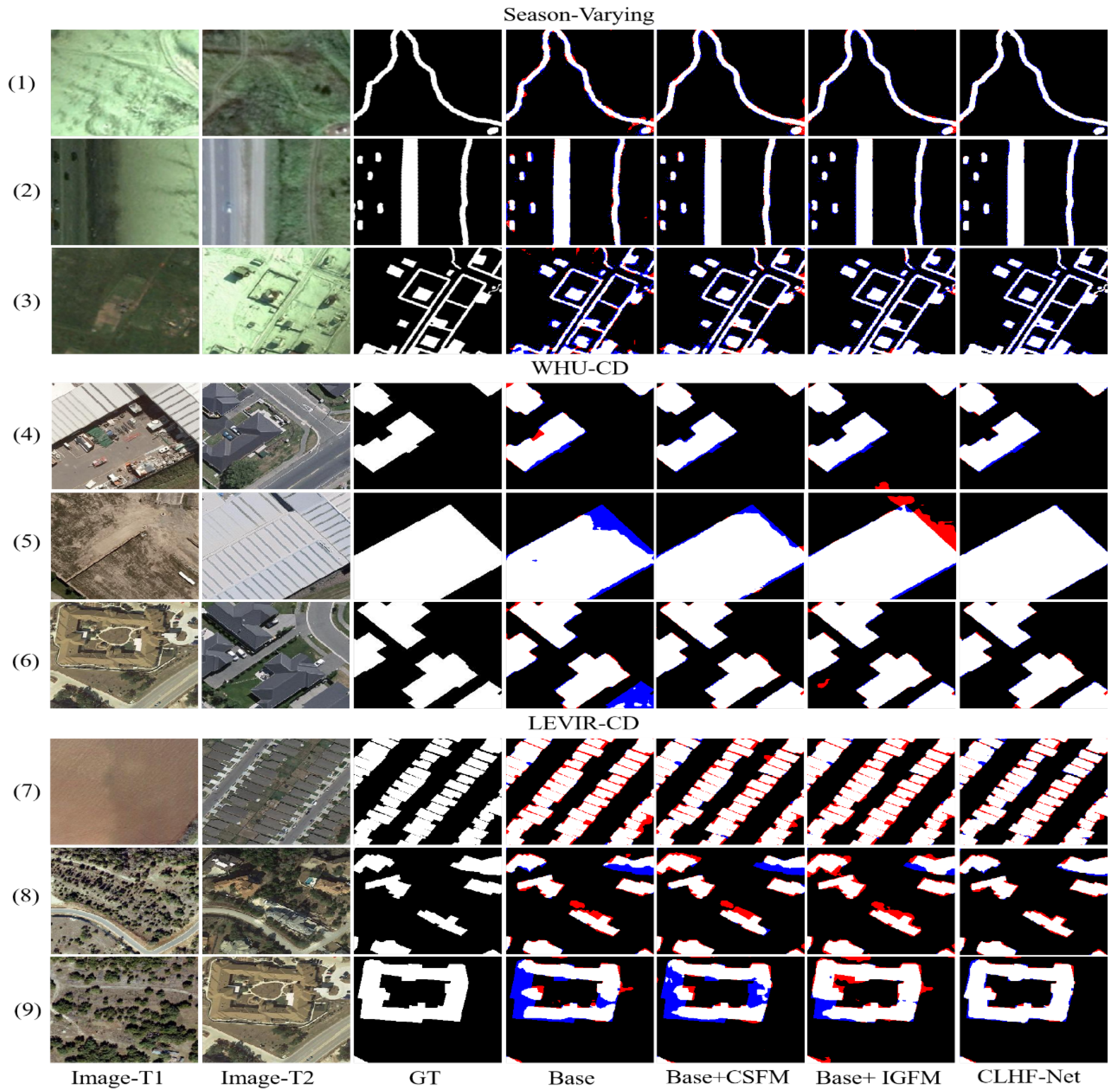
4.4.1. Evaluation for the Season-Varying Dataset

As can be seen from the data in Table 4, the proposed CLHF-Net has the best overall performance. The highest scores were obtained for OA, recall, F1, and Kappa with 99.33%, 98.90%, 97.19%, and 96.80%, respectively. Compared with other methods, CLHF-Net achieved significant improvements of at least 0.24%, 3.0%, 1.03%, and 1.15% on OA, recall, F1, and Kappa, respectively.
Specifically, CD-Net performs relatively poorly in the four metrics, scoring 15.3% and 3.48% lower than CLHF-Net in F1 and OA scores, respectively. Compared to FC-EF, FC-Siam-Conc and FC-Siam-Diff achieved better performance. Among these three baselines, FC-Siam-diff has the best performance, scoring 0.84% and 0.14% higher than FC-Siam-conc on F1 and OA, respectively. STANet achieves F1 and Kappa scores of 91.56% and 90.40%, respectively, which are 1.26% and 1.19% higher than DSIFN, respectively. SNUNet-CD/48 ranked second among all evaluated metrics. On the whole, the proposed CLHF-Net reached the highest level.
The season-varying dataset has multiple types of changes, mainly related to building changes, road changes, vehicle changes, and land changes. To directly compare the performance of the different methods, we visualized the test results. Figure 5 shows several typical results from the qualitative analysis. The detection results of CD-Net are similar to those of FC-EF, with many missed and false detection regions and poor CD performance. The detection results of FC-Siam-Conc and FC-Siam-diff are better than those of FC-EF, but there are still many missed and false detection cases, and the overall performance is not satisfactory. It can be seen from Figure 5 that the above four methods can obtain better detection results only when the change area is larger (Figure 5a,c). However, they do not perform well for smaller change regions and more complex scenes (Figure 5b,d,e). The DASNet, DSIFN, and STANet are better at detecting small change regions and obtain more complete and accurate change regions for the detection results. However, they still have false positives and false negatives in detecting some very small target regions or edges, as shown in the red and blue regions in Figure 5b,d,e. The proposed CLHF-Net can better label the change region and accurately detect the edges of the change region. It can be seen that the change maps produced by CLHF-Net retain the real shape of changing objects with more complete boundaries and successfully filter out some irrelevant factors compared to other models. CLHF-Net can correctly detect not only large changing regions (Figure 5a,c) but also distinguish small changing regions shown in Figure 5b,e,d (narrow roads, vehicles). Compared with other methods, the CLHF-Net has only a small number of red and blue areas in the test result samples, which also indicates that the change map of the proposed network is more in line with the ground reality.

4.4.2. Evaluation for the WHU-CD Dataset

According to the data in Table 5, there is little difference in performance between the methods with FCN as the baseline. The dual-attention-based DASNet performs slightly better than DSIFN and STANet. This may be because the weighted double-margin contrastive loss (WDMC) used by DASNet can address the sample imbalance. The proposed CLHF-Net achieves the best score in all evaluation metrics compared to other comparison methods. Compared with the second-best SNUNet-CD/48, the proposed method obtained 0.28%, 2.24%, 2.5%, and 2.91% gains in OA, R, F1, and Kappa, respectively. This gain is attributed to our channel multigroup feature fusion strategy, which fully considers the different importance of channel group features and reduces the excessive attention to irrelevant information and the neglect of important information. It also effectively takes advantage of the attention and greatly improves the network performance. In addition, the use of a guidance fusion strategy to fuse different layers of features in the decoding stage further improves the network performance.
For a visual comparison, Figure 6 shows some typical CD results for the test samples of the WHU-CD dataset. As shown in Figure 6a–e, there are many missed and false detection regions in the test results of CD-Net and FC series methods. The performance of DASNet is improved after the introduction of dual attention, and there are fewer missed and false detections compared to FC series methods. However, as shown in Figure 6a–c, DASNet is not effective in integrity detection of change regions and CD of small targets. The performance of STANet and DSIFN is similar, but there are still missed and false detection regions in their test results. In addition, as shown in Figure 6d,e, STANet and DSIFN still have significant shortcomings in terms of consistency with GT. In terms of consistency with GT, SNUNet-CD/48 and the proposed CLHF-Net obtain better visual performance. However, as shown in Figure 6d, CLHF-Net can detect smaller change regions compared to the SNUNet-CD/48 method. It produces change maps with clearer and more accurate boundaries. It is worth noting that the detection of very small change regions in Figure 6b is still deficient for all methods. This also indicates that it is important to improve the network’s ability to detect very small object regions in future work.

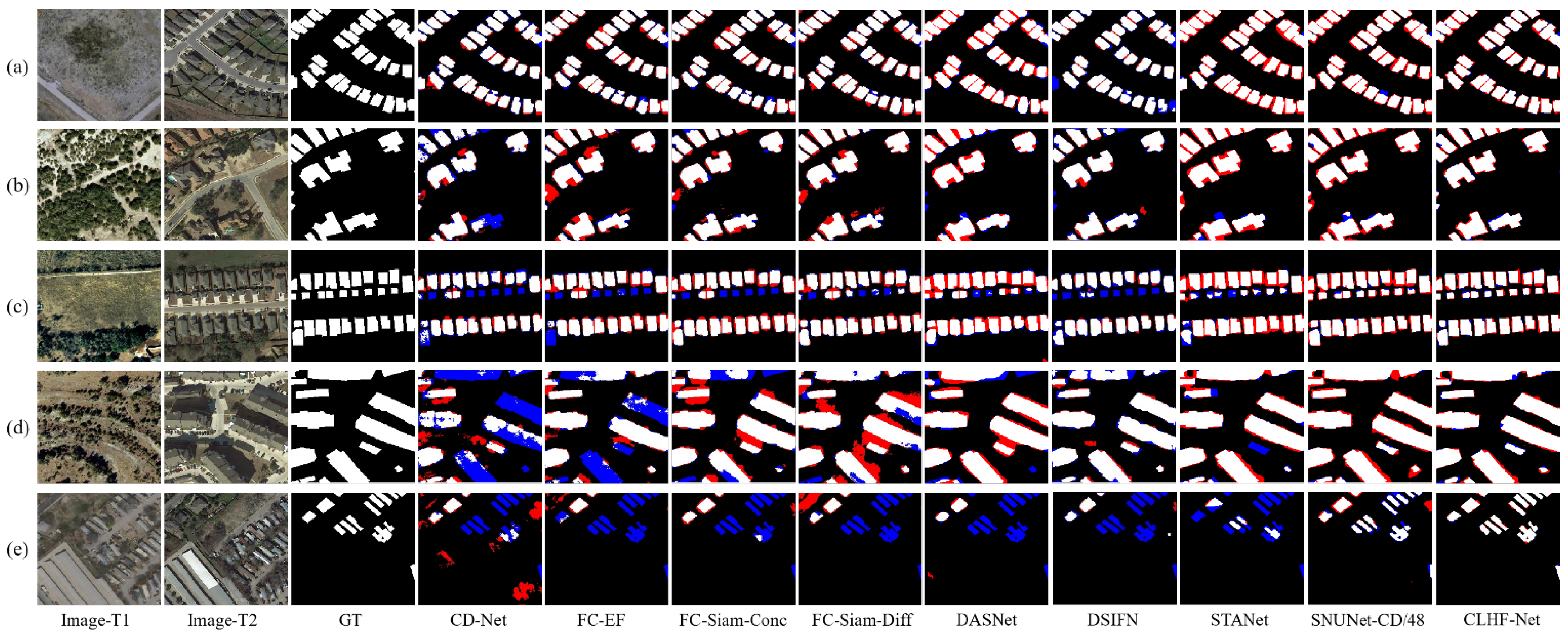
4.4.3. Evaluation for the LEVIR-CD Dataset

As shown in Table 6, the performance difference between FC-EF, FC-Siam-Conc, and FC-Siam-Diff is not significant, and the best performance is in FC-Siam-Diff, which has OA, P, R, F1, and Kappa scores of 98.33%, 83.31%, 84.15%, 83.73%, and 82.85%, respectively. Based on the dual attention DASNet, the F1 and OA scores improved by about 0.4% and 0.87% compared to the three baselines of FCN. The performance of STANet is better than the methods mentioned above. This may be because STANet improves the network performance by introducing attention while paying more attention to multi-scale information. The OA, R, F1, and Kappa scores of the proposed CLHF-Net improved 0.22%, 6.39%, 3.03%, and 3.14%, respectively, over the second-best SNUNet-CD/48, and only the score of P (89.15%) was slightly lower than its score (89.46%).
Figure 7 shows five selected sets of images of the test results. Among these detection results, there are still significant false and missed regions in the detection results of the CD-Net and FC-EF methods (Figure 7b–e). The buildings in the samples in Figure 7c, and e are compactly adjacent to each other without clearer boundaries, which poses a challenge to the CD task, so the detection results of the other methods in these two samples are not satisfactory except for SNUNet-CD/48 and the proposed CLHF-Net. Although SNUNet-CD/48 can locate the change regions, the detection of the edge information is not completely correct. In the visualization map, CLHF-Net has fewer red labeled regions, so the proposed CLHF-Net is more accurate than other methods. For the densely distributed change regions with small targets in Figure 7e, the CLHF-Net has less error and can accurately detect and distinguish multiple densely distributed change regions. CLHF-Net shows a better detection effect for the region with complex edges in Figure 7c.

5. Discussion

In order to verify the efficiency of the different innovation modules, further experiments are developed in this section to discuss the validity and effectiveness of each module in the proposed approach.

5.1. Ablation Study

To verify the effectiveness of our proposed method and the individual modules, we performed an ablation study. First, we added each module separately to the baseline and finally incorporated all modules, including CSFM and IGFM. The structure of the baseline is shown in Figure 8, including three parts of the Siamese ResNet18 backbone, feature aggregation, and pixel classifier. The Convs-N (N denotes 1, 2, 3, 4) and the pixel classifier in Figure 8 are the same as in the proposed CLHF-Net. It should be noted that the number of channels of input features for each Convs-N in the baseline is not the same as that of each Convs-N in CLHF-Net. The results of the quantitative analysis are shown in Table 7.
Compared with other methods, the baseline method proposed in this paper has shown better performance. On the season-varying dataset, the F1 value of the baseline method is 3.55% higher than the third ranked STANet in terms of performance and 1.05% lower than the second ranked SNUNet-CD/48. The baseline method also performs well on the other two datasets. This indicates that the baseline method designed in this paper outperforms most of the comparison methods.
CSFM brings 1.39%, 3.42%, and 1.53% improvement in F1 for the baseline on the season-varying, WHU-CD, and LEVIR-CD datasets, respectively. In addition, there were also significant improvements in other metric values for CSFM. These results demonstrate the effectiveness of the channel-split feature fusion strategy. The IGFM brings 0.98%, 2.83%, and 1.95% improvement in F1 for the baseline on the three datasets, respectively. The gains of IGFM on the season-varying and LEVIR-CD datasets were higher than those of CSFM. This shows that the feature fusion approach and feature interaction guidance fusion strategy we have designed are effective.
The qualitative analysis of this ablation study is shown in Figure 9. It can be seen that all models performed well on the season-varying dataset (samples (1–3)). The proposed CLHF-Net correctly distinguishes and detects the changed regions, and there are almost no missed and false detections. In samples (4–6) (WHU-CD dataset), the baseline method performs poorly and has more missed regions. The Base+CSFM method improves the performance significantly, has few missed and false regions in these three samples, and essentially detects the changed regions correctly. The Base+IGFM method also performs well but has false detection. The performance of the Base+IGFM method is also good, but there are false detections. The performance of the CLHF-Net is better than the comparison methods, except for a small area that was missed detection in the sample (4). In samples (7–9) (LEVIR-CD dataset), the change scenes are more complex, which challenged these methods. The Base and Base+CSFM methods do not perform well. The Base+IGFM method performs second only to the CLHF-Net method. However, the Base+IGFM method still has significant missed and false detection regions. The CLHF-Net method still performs well on the LEVIR-CD dataset, and although there are few false detection regions, the change regions are detected correctly.

5.2. Effectiveness of CSFM

The proposed CSFM consists of a channel splitting branch (CSB), IFU, and feature aggregation branch (FAB). Here, we focus on the CSB and IFU. We verify the effectiveness of both through experiments.

5.2.1. Analysis of Channel Splitting Branch (CSB)

The analysis of the channel splitting branch (CSB) consists of two main aspects. In the first aspect, we analyze how many channel groups it is most efficient to split the feature map into. In the second aspect, we analyze whether the channel splitting strategy is effective.
For the first aspect, we performed a comparison experiment. We split the feature map into a different number of channel group features. Specifically, we set c in CSFM (shown in Figure 2) to 16, 32, and 64, respectively. Table 8 shows the comparison results in the three datasets. The results in Table 5 show that the network performance is best when c is 16.
For the second aspect, to demonstrate the effectiveness of CSB, another experiment was conducted. In this experiment, two input features were not processed by splitting. The IFU and FAB operations were used for the two input features. The data in Table 9 record the results obtained for this experiment and for CLHF-Net with CSB. It can be demonstrated that the performance of the model without CSB is not as good as the performance of CLHF-Net. This indicates that our SCB is effective.

5.2.2. Analysis of IFU

To verify the contribution of IFU to CSB and the whole network, we designed the structure shown in Figure 10b to compare with our proposed IFU. The structure is shown in Figure 10b, which we named NIFU. It can be seen, in NIFU, we apply the element-wise multiplication operation to the CA map and input of CA, which is different from IFU. This design is to demonstrate that our adoption of the interactive fusion strategy is effective.
From Table 10, we can see that the F1 and OA scores of CLHF-Net with IFU are improved compared to CLHF-Net with NIFU. In the season-varying dataset, F1 and OA are improved by 0.96% and 0.21%, respectively. In the WHU-CD dataset, F1 and OA are improved by 1.19% and 0.11%, respectively. In the LEVIR-CD dataset, F1 and OA are improved by 1.53% and 0.14%, respectively. This demonstrated that the IFU we designed was effective.

5.3. Effectiveness of IGFM

To evaluate the validity of IGFM, we designed a comparison module. Specifically, the comparison module is almost as similar in structure to IGFM, the only difference is that the comparison module no longer uses the interaction guidance strategy. We named the comparison module FFM. In FFM, we apply the channel-wise multiplication operation to the map output by the sigmoid function and the original input. Table 11 records the results of CLHF-Net with IGFM and CLHF-Net with FFM for the three datasets.
As shown in Table 11, the IGFM we designed has a significant improvement compared to the FFM in the three datasets. In the season-varying, WHU-CD, and LEVIR-CD datasets, F1 improved by 0.73%, 1.27%, and 1.65%, respectively. In addition, OA gained 0.16%, 0.12%, 6.92%, and 0.17%, respectively. This interaction guidance strategy is helpful for network performance improvement in different datasets.

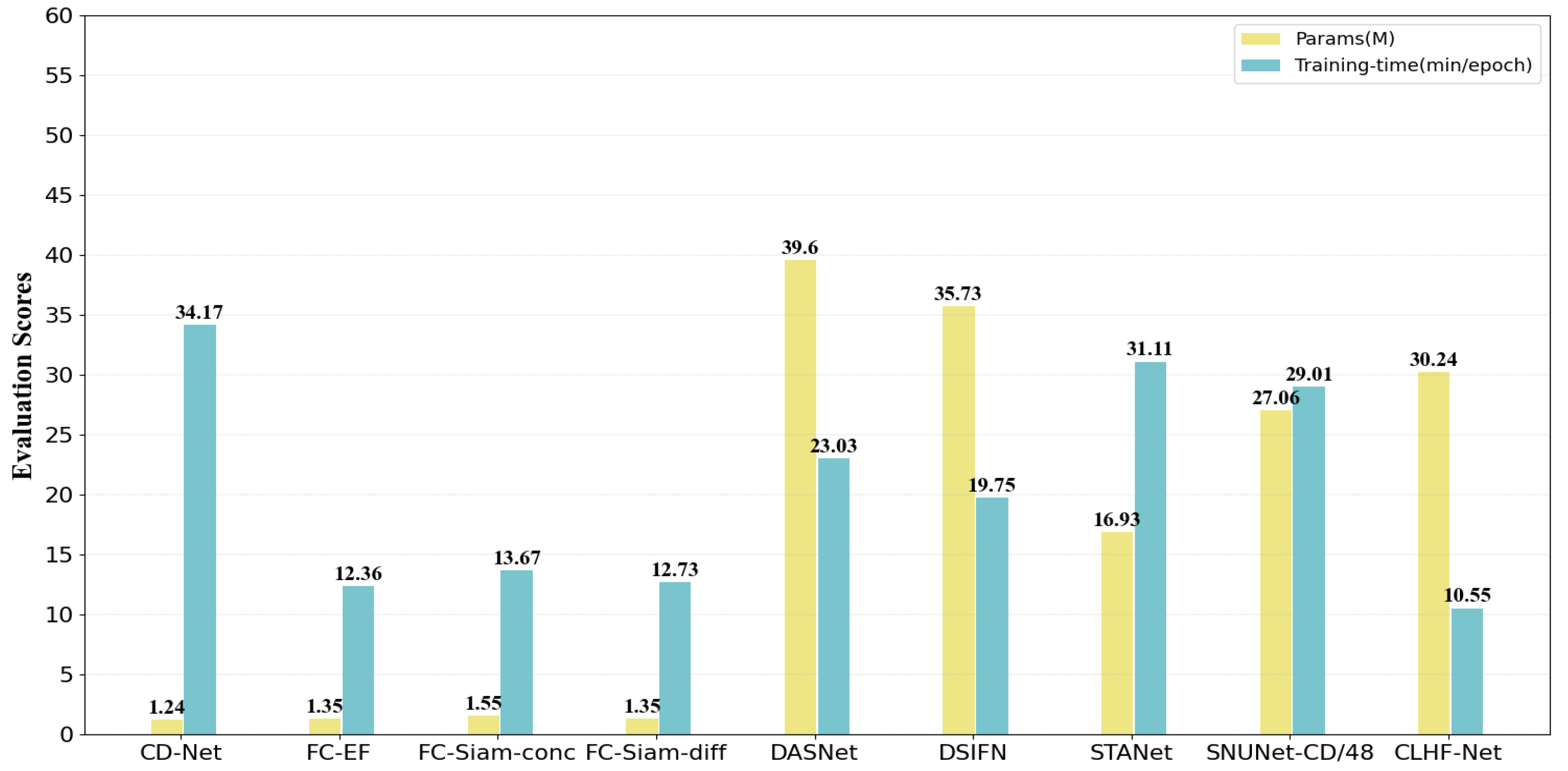
5.4. Efficiency Analysis of the Proposed Network

To analyze the efficiency of the different methods with respect to the number of parameters and training speed under the same experimental conditions (hardware computing power), we compared the proposed method with other methods. The quantitative indicators performed for the evaluation were the number of parameters (take M as the unit) and the training time for one epoch (take min/epoch as the unit). Figure 11 shows the efficiency of all methods.
As can be seen in Figure 11, DASNet has the most model parameters and CD-Net consumes the longest time to complete a training epoch. Although CD-Net has the least number of parameters, it has a significant disadvantage at the training speed, which makes it limited in practical applications. FC series methods have fewer parameters, but they have no significant advantage in training speed. In addition, as we can see in the previous analysis of the CD results, they are as inefficient as other methods (only better than CD-Net). DSIFN has only fewer parameters than DASNet, but it is better than STANet and SNUNet-CD/48 in terms of training speed. From the results in Section 3, it performs well in the CD task. The number of parameters of STANet and SNUNet-CD/48 is less than the proposed method, but the training time is more than the proposed approach. The training speed of the CLHF-Net is the fastest, and the time to train one epoch is reduced by 12.30% compared to SNUNet-CD/48. The above facts show that the proposed method has a good trade-off between the best detection results and efficiency.
While the proposed CLHF-Net outperforms other methods and has high efficiency, it has some potential limitations. As can be seen in Figure 11, the computational complexity of CLHF-Net is relatively high with a parameter count of 30.24 M. This is undesirable when equipment resources are limited and may be discouraging for practical applications. Therefore, in future work, it is hoped that the size of the network model can be reduced by employing model compression techniques such as pruning and knowledge distillation [60,61], making the network lightweight.

6. Conclusions

In this article, a novel convolutional neural network (CLHF-Net) with symmetric structure for CD of RS images is proposed. To research the importance of different channel group features, we designed CSFM, which consists of three parts, namely CSB, IFU, and FAB. The CSFM weights and fuses channel features of different importance to produce the higher quality difference feature maps. Considering that shallow and deep features have different semantic information, a feature interaction guidance fusion strategy is used in order to fuse features of different layers well. This strategy is to introduce the deep semantic information into the shallow features and the detailed information of the shallow features into the deep features. This eliminates the redundant spatial information in the shallow features, while compensating for the detailed information in the deep features. Compared with existing SOTA methods, the proposed CLHF-Net achieves superior performance on OA, F1, and Kappa scores of three benchmark datasets, which indicates that it achieves a more comprehensive performance. From the qualitative analysis, more pixels are accurately detected in the change maps obtained by CLHF-Net, while there are relatively fewer unpredicted changes and false positives. The experimental results demonstrate the effectiveness and generalization ability of CLHF-Net. The best performance in detecting large change regions and small change regions proves the effectiveness and robustness of CLHF-Net.
However, it should be noted that, as shown in Figure 11, although the proposed model has an advantage in terms of training speed, it cannot be ignored that the method proposed in this paper is not superior in terms of number of parameters, which reaches 30.24 M. This has potential limitations for its practical application in the future. Therefore, in future work, we hope that the network can be made lightweight by using some model compression techniques.

Author Contributions

Conceptualization, J.M.; methodology, J.M.; software, D.L. and Y.L.; validation, J.M. and D.L.; formal analysis, G.S. and Y.L.; investigation, G.S. and Y.L.; resource, J.M. and D.L.; data curation, J.M. and D.L.; writing—original draft preparation, J.M.; writing—review and editing, G.S., J.M., D.L. and Y.L. All authors have read and agreed to the published version of the manuscript.

Funding

This work was supported by the National Natural Science Foundation of China (No. 12061072) and the Natural Science Foundation of China (No. 62162059).

Institutional Review Board Statement

Not applicable.

Informed Consent Statement

Not applicable.

Data Availability Statement

The season-varying, WHU-CD, and LEVIR-CD datasets are openly available at https://drive.google.com/fifile/d/1GX656JqqOyBi_Ef0w65kDGVto-nHrNs9 (accessed on 28 March 2022), http://gpcv.whu.edu.cn/data/building_dataset.html (accessed on 28 March 2022), https://justchenhao.github.io/LEVIR/ (accessed on 28 March 2022), respectively.

Conflicts of Interest

The authors declare no conflict of interest.

Abbreviations

The following abbreviations are used in this manuscript:
CDChange Detection
RSRemote Sensing
CLHF-NetChannel-Level Hierarchical Feature Fusion Network
CSFMChannel-Split Feature Fusion Module
IGFMInteraction Guidance Fusion Module
CNNConvolutional Neural Network
FCNFully Convolutional Neural Network
CSBChannel Splitting Branch
IFUInteraction Fusion Unit
FABFeature Aggregation Branch
DLDeep Learning
ICAIndependent Component Analysis
MADMultivariate Alteration Detection
CVAChange Vector Analysis
C 2 VA Compressed Change Vector Analysis
HSCVAHierarchical Spectral Change Vector Analysis
S 2 CVA Sequential Spectral Change Vector Analysis
SVDSingular Value Decomposition
PCAPrincipal Component Analysis
TMFTriple Markov Field
FC-EFFully Convolutional Early Fusion
FC-Siam-concFully Convolutional Siamese Concatenation
FC-Siam-diffFully Convolutional Siamese Difference
DSIFNDeeply Supervised Image Fusion Network
ADS-NetAttention Mechanism-based Deep Supervision Network
HDFNetHierarchical Dynamic Fusion Network
CLNetU-Net based Cross-Layer Convolutional Neural Network
STANetSpatial–Temporal Attention Neural Network
AGCDetNetAttention-based End-to-End Change Detection Network
GTGround Truth
TPTrue Positive
TNTrue Negative
FPFalse Positive
FNFalse Negative

References

  1. Bruzzone, L.; Bovolo, F. A Novel Framework for the Design of Change-Detection Systems for Very-High-Resolution Remote Sensing Images. Proc. IEEE 2013, 101, 609–630. [Google Scholar] [CrossRef]
  2. Zhu, X.X.; Tuia, D.; Mou, L.; Xia, G.; Zhang, L.; Xu, F.; Fraundorfer, F. Deep Learning in Remote Sensing: A Comprehensive Review and List of Resources. IEEE Geosci. Remote Sens. Mag. 2017, 5, 8–36. [Google Scholar] [CrossRef] [Green Version]
  3. Khelififi, L.; Mignotte, M. Deep Learning for Change Detection in Remote Sensing Images: Comprehensive Review and Meta-Analysis. IEEE Access. 2020, 8, 126385–126400. [Google Scholar] [CrossRef]
  4. Shi, W.; Zhang, M.; Zhang, R.; Chen, S.; Zhan, Z. Change Detection Based on Artificial Intelligence: State-of-the-Art and Challenges. Remote Sens. 2020, 12, 1688. [Google Scholar] [CrossRef]
  5. Ma, B.; Ban, X.; Huang, H.; Chen, Y.; Liu, W.; Zhi, Y. Deep Learning-Based Image Segmentation for Al-La Alloy Microscopic Images. Symmetry 2018, 10, 107. [Google Scholar] [CrossRef] [Green Version]
  6. Fu, H.; Song, G.; Wang, Y. Improved YOLOv4 Marine Target Detection Combined with CBAM. Symmetry 2021, 13, 623. [Google Scholar] [CrossRef]
  7. Sun, Y.; Bi, F.; Gao, Y.; Chen, L.; Feng, S. A Multi-Attention UNet for Semantic Segmentation in Remote Sensing Images. Symmetry 2022, 14, 906. [Google Scholar] [CrossRef]
  8. Zhang, C.; Yue, P.; Tapete, D.; Jiang, L.; Shangguan, B.; Huang, L.; Liu, G. A deeply supervised image fusion network for change detection in high resolution bi-temporal remote sensing images. ISPRS J. Photogramm. Remote Sens. 2020, 166, 183–200. [Google Scholar] [CrossRef]
  9. Peng, D.; Zhang, Y.; Guan, H. End-to-end change detection for high resolution satellite images using improved unet++. Remote Sens. 2019, 11, 1382. [Google Scholar] [CrossRef] [Green Version]
  10. Daudt, R.C.; Saux, B.L.; Boulch, A. Fully Convolutional Siamese Networks for Change Detection. In Proceedings of the 25th IEEE International Conference on Image Processing (ICIP), Athens, Greece, 7–10 October 2018; pp. 4063–4067. [Google Scholar]
  11. Shelhamer, E.; Long, J.; Darrell, T. Fully Convolutional Networks for Semantic Segmentation. IEEE Trans. Pattern Anal. Mach. Intell. 2017, 39, 640–651. [Google Scholar] [CrossRef]
  12. Zhang, C.; Wei, S.; Ji, S.; Lu, M. Detecting large-scale urban land cover changes from very high-resolution remote sensing images using CNN-based classification. ISPRS Int. J. Geo-Inf. 2019, 8, 89. [Google Scholar] [CrossRef] [Green Version]
  13. Zhang, H.; Gong, M.; Zhang, P.; Su, L.; Shi, J. Feature-level change detection using deep representation and feature change analysis for multispectral imagery. IEEE Geosci. Remote Sens. Lett. 2016, 13, 1666–1670. [Google Scholar] [CrossRef]
  14. Zhao, Q.; Ma, J.; Gong, M.; Li, H.; Zhan, T. Three-class change detection in synthetic aperture radar images based on deep belief network. J. Comput. Theor. Nanosci. 2016, 13, 3757–3762. [Google Scholar] [CrossRef]
  15. Wang, Q.; Yuan, Z.; Du, Q.; Li, X. GETNET: A general end-to-end 2-D CNN framework for hyperspectral image change detection. IEEE Trans. Geosci. Remote Sens. 2019, 57, 3–13. [Google Scholar] [CrossRef] [Green Version]
  16. Hussain, M.; Chen, D.; Cheng, A.; Wei, H.; Stanley, D. Change detection from remotely sensed images: From pixel-based to object-based approaches. ISPRS J. Photogramm. Remote Sens. 2013, 80, 91–106. [Google Scholar] [CrossRef]
  17. Tewkesbury, A.P.; Comber, A.J.; Tate, N.J.; Lamb, A.; Fisher, P.F. A critical synthesis of remotely sensed optical image change detection techniques. Remote Sens. Environ. 2015, 160, 1–14. [Google Scholar] [CrossRef] [Green Version]
  18. Quarmby, N.A.; Cushnie, J.L. Monitoring urban land cover changes at the urban fringe from SPOT HRV imagery in south-east England. Int. J. Remote Sens. 1989, 10, 953–963. [Google Scholar] [CrossRef]
  19. Howarth, P.J.; Wickwareg, M. Procedures for change detection using Landsat digital data. Int. J. Remote Sens. 1981, 2, 277–291. [Google Scholar] [CrossRef]
  20. Ludeke, A.K.; Maggio, R.; Reid, L.M. An Analysis of Anthropogenic Deforestation Using Logistic Regression and GIS. J. Environ. Manag. 1990, 31, 247–259. [Google Scholar] [CrossRef]
  21. Zhang, J.; Wang, R. Multi-temporal remote sensing change detection based on independent component analysis. Int. J. Remote Sens. 2006, 27, 2055–2061. [Google Scholar] [CrossRef]
  22. Nielsen, A.A. The Regularized Iteratively Reweighted MAD Method for Change Detection in Multi- and Hyperspectral Data. IEEE Trans. Image Process. 2007, 16, 463–478. [Google Scholar] [CrossRef] [PubMed] [Green Version]
  23. Bovolo, F.; Bruzzone, L. A theoretical framework for unsupervised change detection based on change vector analysis in the polar domain. IEEE Trans. Geosci. Remote Sens. 2007, 45, 218–236. [Google Scholar] [CrossRef] [Green Version]
  24. Bovolo, F.; Marchesi, S.; Member, S. A framework for automatic and unsupervised detection of multiple changes in multitemporal images. IEEE Trans. Geosci. Remote Sens. 2012, 50, 2196–2212. [Google Scholar] [CrossRef]
  25. Liu, S.; Bruzzone, L.; Bovolo, F.; Du, P. Hierarchical unsupervised change detection in multi-temporal hyperspectral images. IEEE Trans. Geosci. Remote Sens. 2015, 53, 244–260. [Google Scholar]
  26. Liu, S.; Bruzzone, L.; Bovolo, F.; Zanetti, M.; Du, P. Sequential spectral change vector analysis for iteratively discovering and detecting multiple changes in hyperspectral images. IEEE Trans. Geosci. Remote Sens. 2015, 53, 4363–4378. [Google Scholar] [CrossRef]
  27. Zanetti, M.; Bruzzone, L. A theoretical framework for change detection based on a compound multiclass statistical model of the difference image. IEEE Trans. Geosci. Remote Sens. 2018, 56, 1129–1143. [Google Scholar] [CrossRef]
  28. Ghaderpour, E.; Vujadinovic, T. Change Detection within Remotely Sensed Satellite Image Time Series via Spectral Analysis. Remote Sens. 2020, 12, 4001. [Google Scholar] [CrossRef]
  29. Ghaderpour, E. JUST: MATLAB and python software for change detection and time series analysis. GPS Solut. 2021, 25, 85. [Google Scholar] [CrossRef]
  30. Masiliūnas, D.; Tsendbazar, N.-E.; Herold, M.; Verbesselt, J. BFAST Lite: A Lightweight Break Detection Method for Time Series Analysis. Remote Sens. 2021, 13, 3308. [Google Scholar] [CrossRef]
  31. Su, J.; Wang, G.; Lin, X.; Liu, D. A Change Detection Algorithm for Man-made Objects Based on Multi-temporal Remote Sensing Images. Acta Autom. Sin. 2008, 34, 13–19. [Google Scholar]
  32. Wang, L.; Li, H. PCA based unsupervised change detection for color satellite images under the quaternion model. In Proceedings of the 2010 International Symposium on Intelligent Signal Processing and Communication Systems (ISPACS 2010), Chengdu, China, 6–8 December 2010; pp. 782–786. [Google Scholar]
  33. Benedek, C.; Sziranyi, T. Change Detection in Optical Aerial Images by a Multilayer Conditional Mixed Markov Model. IEEE Trans. Geosci. Remote Sens. 2009, 47, 3416–3430. [Google Scholar] [CrossRef] [Green Version]
  34. Inglada, J.; Mercier, G. A New Statistical Similarity Measure for Change Detection in Multitemporal SAR Images and Its Extension to Multiscale Change Analysis. IEEE Trans. Geosci. Remote Sens. 2011, 45, 1432–1445. [Google Scholar] [CrossRef] [Green Version]
  35. Wang, F.; Wu, Y.; Zhang, Q.; Zhang, P.; Li, M.; Lu, Y. Unsupervised Change Detection on SAR Images Using Triplet Markov Field Mode. IEEE Geosci. Remote Sens. Lett. 2013, 10, 697–701. [Google Scholar] [CrossRef]
  36. Wang, X.; Liu, S.; Du, P.; Liang, H.; Xia, J.; Li, Y. Object-Based Change Detection in Urban Areas from High Spatial Resolution Images Based on Multiple Features and Ensemble Learning. Remote Sens. 2018, 10, 276. [Google Scholar] [CrossRef] [Green Version]
  37. Zhang, Y.; Peng, D.; Huang, X. Object-based change detection for VHR images based on multiscale uncertainty analysis. IEEE Geosci. Remote Sens. Lett. 2017, 15, 13–17. [Google Scholar] [CrossRef]
  38. Tan, K.; Zhang, Y.; Wang, X.; Chen, Y. Object-Based Change Detection Using Multiple Classifiers and Multi-Scale Uncertainty Analysis. Remote Sens. 2019, 11, 359. [Google Scholar] [CrossRef] [Green Version]
  39. Wiratama, W.; Sim, D. Fusion network for change detection of high-resolution panchromatic imagery. Appl. Sci. 2019, 9, 1441. [Google Scholar] [CrossRef] [Green Version]
  40. Woo, S.; Park, J.; Lee, J.-Y.; Kweon, I.S. CBAM: Convolutional Block Attention Module. In Proceedings of the Computer Vision—ECCV 2018, Munich, Germany, 8–14 September 2018; pp. 3–19. [Google Scholar]
  41. Lei, Y.; Peng, D.; Zhang, P.; Ke, Q.; Li, H. Hierarchical paired channel fusion network for street scene change detection. IEEE Trans. Image Process. 2020, 30, 55–67. [Google Scholar] [CrossRef]
  42. Fang, S.; Li, K.; Shao, J.; Li, Z. SNUNet-CD: A Densely Connected Siamese Network for Change Detection of VHR Images. IEEE Geosci. Remote Sens. Lett. 2021, 19, 1–5. [Google Scholar] [CrossRef]
  43. Wang, D.; Chen, X.; Jiang, M.; Du, S.; Xu, B.; Wang, J. ADS-Net: An Attention-Based deeply supervised network for remote sensing image change detection. Int. J. Appl. Earth Obs. Geoinf. 2021, 101, 102348. [Google Scholar]
  44. Zhang, Y.; Fu, L.; Li, Y.; Zhang, Y. HDFNet: Hierarchical Dynamic Fusion Network for Change Detection in Optical Aerial Images. Int. J. Remote Sens. 2021, 13, 1440. [Google Scholar] [CrossRef]
  45. Hou, X.; Bai, Y.; Li, Y.; Shang, C.; Shen, Q. High-resolution triplet network with dynamic multiscale feature for change detection on satellite images. ISPRS J. Photogramm. Remote Sens. 2021, 177, 103–115. [Google Scholar] [CrossRef]
  46. Zheng, Z.; Wan, Y.; Zhang, Y.; Xiang, S.; Peng, D.; Zhang, B. CLNet: Cross-layer convolutional neural network for change detection in optical remote sensing imagery. ISPRS J. Photogramm. Remote Sens. 2021, 175, 247–267. [Google Scholar] [CrossRef]
  47. Yang, K.; Xia, G.-S.; Liu, Z.; Du, B.; Yang, W.; Pelillo, M.; Zhang, L. Asymmetric Siamese Networks for Semantic Change Detection in Aerial Images. IEEE Trans. Geosci. Remote Sens. 2021, 60, 1–18. [Google Scholar] [CrossRef]
  48. Chen, J.; Yuan, Z.; Peng, J.; Chen, L.; Huang, H.; Zhu, J.; Liu, Y.; Li, H. DASNet: Dual attentive fully convolutional siamese networks for change detection of high-resolution satellite images. IEEE J. Sel. Top. Appl. Earth Obs. Remote Sens. 2020, 14, 1194–1206. [Google Scholar] [CrossRef]
  49. Chen, H.; Shi, Z. A Spatial-Temporal Attention-Based Method and a New Dataset for Remote Sensing Image Change Detection. Remote Sens. 2020, 12, 1662. [Google Scholar] [CrossRef]
  50. Song, K.; Jiang, J. AGCDetNet:An Attention-Guided Network for Building Change Detection in High-Resolution Remote Sensing Images. IEEE J. Sel. Top. Appl. Earth Obs. Remote Sens. 2021, 14, 4816–4831. [Google Scholar] [CrossRef]
  51. Li, G.; Liu, Z.; Chen, M.; Bai, Z.; Lin, W.; Ling, H. Hierarchical Alternate Interaction Network for RGB-D Salient Object Detection. IEEE Trans. Image Process. 2021, 30, 3528–3542. [Google Scholar] [CrossRef]
  52. Shi, C.; Zhang, X.; Wang, L. A Lightweight Convolutional Neural Network Based on Channel Multi-Group Fusion for Remote Sensing Scene Classification. Remote Sens. 2022, 14, 9. [Google Scholar] [CrossRef]
  53. Wei, H.; Chen, R.; Yu, C.; Yang, H.; An, S. BASNet: A Boundary-Aware Siamese Network for Accurate Remote Sensing Change Detection. IEEE Geosci. Remote Sens. Lett. 2021, 19, 1. [Google Scholar] [CrossRef]
  54. Chen, H.; Qi, Z.; Shi, Z. Remote Sensing Image Change Detection with Transformers. IEEE Trans. Geosci. Remote Sens. 2021, 60, 1–14. [Google Scholar] [CrossRef]
  55. Xu, J.; Luo, C.; Chen, X.; Wei, S.; Luo, Y. Remote Sensing Change Detection Based on Multidirectional Adaptive Feature Fusion and Perceptual Similarity. Remote Sens. 2021, 13, 3053. [Google Scholar] [CrossRef]
  56. He, K.; Zhang, X.; Ren, S.; Sun, J. Deep residual learning for image recognition. In Proceedings of the IEEE Conference on Computer Vision and Pattern Recognition (CVPR), Las Vegas, NV, USA, 27–30 June 2016; pp. 770–778. [Google Scholar]
  57. Lebedev, M.; Vizilter, Y.V.; Vygolov, O.; Knyaz, V.; Rubis, A.Y. Change Detection in Remote Sensing Images Using Conditional Adversarial Networks. Int. Arch. Photogramm. Remote Sens. Spat. Inf. Sci. 2018, 42, 565–571. [Google Scholar] [CrossRef] [Green Version]
  58. Ji, S.; Wei, S.; Lu, M. Fully convolutional networks for multisource building extraction from an open aerial and satellite imagery data set. IEEE Trans. Geosci. Remote Sens. 2018, 57, 574–586. [Google Scholar] [CrossRef]
  59. Alcantarilla, P.F.; Simon, S.; Germán, R.; Roberto, A.; Riccardo, G. Street-view change detection with deconvolutional networks. Auton. Robot. 2018, 42, 1301–1322. [Google Scholar] [CrossRef]
  60. Li, H.; Kadav, A.; Durdanovic, I.; Samet, H.; Graf, H.P. Pruning filters for efficient convnets. arXiv 2016, arXiv:1608.08710. [Google Scholar]
  61. Vadera, M.P.; Marlin, B.M. Challenges and Opportunities in Approximate Bayesian Deep Learning for Intelligent IoT Systems. arXiv 2021, arXiv:2112.01675. [Google Scholar]
Figure 1. Channel-level hierarchical feature fusion network (CLHF-Net).
Symmetry 14 01138 g001
Figure 2. Channel-split feature fusion module (CSFM). The figure shows the detailed structure of CSFM-1. is the channel-wise multiplication, is the element-wise summation, is the element-wise multiplication, and © is the concatenation operation.
Symmetry 14 01138 g002
Figure 3. Interaction guidance fusion module (IGFM).
Symmetry 14 01138 g003
Figure 4. The structure of the classifier.
Symmetry 14 01138 g004
Figure 5. Visualization of CD results on dataset season-varying. (ad) represent the changes of roads and buildings on the ground surface. (e) represents the change of buildings on the ground surface. The white indicates true positive. Black indicates true negative. Red indicates false positive. Blue indicates false negative.
Symmetry 14 01138 g005
Figure 6. Visualization of CD results on dataset WHU-CD. (ae) represent the changes of the buildings on the ground surface. The white indicates true positive. Black indicates true negative. Red indicates false positive. Blue indicates false negative.
Symmetry 14 01138 g006
Figure 7. Visualization of CD results on dataset LEVIR-CD. (ae) represent the changes of the buildings on the ground surface. The white indicates true positive. Black indicates true negative. Red indicates false positive. Blue indicates false negative.
Symmetry 14 01138 g007
Figure 8. Detailed architecture of the baseline.
Symmetry 14 01138 g008
Figure 9. Visualization of CD results for different models on three datasets. (1–3) indicate samples from Season-Varying dataset, (4–6) indicate samples from WHU-CD dataset, and (7–9) indicate samples from LEVIR-CD dataset. The white indicates true positive. Black indicates true negative. Red indicates false positive. Blue indicates false negative.
Symmetry 14 01138 g009
Figure 10. The structure in (a) is the IFU in our network, and the structure in (b) is the NIFU.
Symmetry 14 01138 g010
Figure 11. Efficiency comparison results on season-varying dataset.
Symmetry 14 01138 g011
Table 1. Description of three datasets.
DatasetsSpatial ResolutionNumber of SamplesSize of Samples
Training SetValidation SetTest Set
Season-Varying3–100 cm/pixel10,00030003000256 × 256
WHU-CD0.2 m/pixel7918987955224 × 224
LEVIR-CD 0.5 m/pixel712010242048256 × 256
Table 2. The detailed explanation of TN, TP, FN, and FP.
True ValuePredicted Value
PositiveNegative
PositiveTPFN
NegativeFPTN
Table 3. The main elements of the contrastive methods.
MethodsArchitectureLoss FunctionPublished Year
CD-Net [59]FCNWeighted cross-entropy loss2018
FC-EF [10]FCNWeighted negative log likelihood loss 2018
FC-Siam-Conc [10]Siamese, FCNWeighted negative log likelihood loss 2018
FC-Siam-Diff [10]Siamese, FCNWeighted negative log likelihood loss 2018
DASNet [48]Siamese, VGG16/ResNet50Weighted double-margin contrastive loss2021
DSIFN [8]Siamese, VGG16Sigmoid binary cross-entropy, dice loss2020
STANet [49]Siamese, ResNet18Batch-balanced contrastive loss2020
SNUNet-CD/48 [42]Siamese, UNet++Weighted cross-entropy loss, dice loss2021
Table 4. Comparison results on season-varying dataset. The bolded data represent the best results.
MethodOA (%)P (%)R (%)F1 (%)Kappa (%)
CD-Net95.8594.0472.5181.8979.59
FC-EF96.0292.3175.5083.0780.84
FC-Siam-Conc96.2594.0575.8483.9681.87
FC-Siam-Diff96.3993.1177.8684.8082.78
DASNet97.5092.2688.0990.1288.69
DSIFN97.6994.9686.0890.3089.21
STANet97.9588.9794.3191.5690.40
SNUNet-CD/4899.0996.3395.9996.1695.65
CLHF-Net99.3395.5498.9097.1996.80
Table 5. Comparison results on WHU-CD dataset. The bolded data represent the best results.
MethodOA (%)P (%)R (%)F1 (%)Kappa (%)
CD-Net98.0277.1884.0080.4579.40
FC-EF98.2480.3484.3982.3181.38
FC-Siam-Conc98.1779.1687.0882.9381.97
FC-Siam-Diff98.3782.7783.9383.3582.49
DASNet97.5092.2688.0990.1288.69
DSIFN98.8688.9487.2988.1187.51
STANet99.0593.3786.5089.8089.30
SNUNet-CD/4899.1388.4290.3989.3988.94
CLHF-Net99.4192.5692.6392.6292.21
Table 6. Comparison results on LEVIR-CD dataset. The bolded data represent the best results.
MethodOA (%)P (%)R (%)F1 (%)Kappa (%)
CD-Net97.8079.5976.5378.0376.88
FC-EF98.0380.4681.0380.7479.70
FC-Siam-Conc98.0878.0086.7982.1781.15
FC-Siam-Diff98.3383.3184.1583.7382.85
DASNet98.3781.4987.9584.6083.74
DSIFN98.6591.7380.8285.9385.22
STANet98.9189.9682.6286.5485.97
SNUNet-CD/4899.0389.4686.3687.8887.38
CLHF-Net99.2589.1592.7590.9190.52
Table 7. Ablation study with different model performance. The bolded data represent the best results.
ModelSeason-VaryingWHU-CDLEVIR-CD
BaselineCSFMIGFMF1 (%)OA (%)F1 (%)OA (%)F1 (%)OA (%)
××95.1198.9388.6498.9287.4298.79
×96.0999.0892.0699.2488.9598.81
×96.5099.1691.4799.1689.3798.87
97.1999.3392.6299.4190.9199.25
Table 8. Ablation study of the value of c.
Method/cSeason-VaryingWHU-CDLEVIR-CD
F1 (%)OA (%)F1 (%)OA (%)F1 (%)OA (%)
CLHF-Net /1697.1999.3392.6299.4190.9199.25
CLHF-Net /3296.3999.1591.2799.2989.4399.11
CLHF-Net /6495.8799.0290.6999.1888.9799.03
Table 9. Ablation study of with/without CSB.
CLHF-NetSeason-VaryingWHU-CDLEVIR-CD
F1 (%)OA (%)F1 (%)OA (%)F1 (%)OA (%)
CLHF-Net -w-CSB97.1999.3392.6299.4190.9199.25
CLHF-Net -w/o-CSB96.2699.1291.2299.2289.1699.01
Table 10. Ablation study of with/without IFU.
CLHF-NetSeason-VaryingWHU-CDLEVIR-CD
F1 (%)OA (%)F1 (%)OA (%)F1 (%)OA (%)
CLHF-Net -w-IFU97.1999.3392.6299.4190.9199.25
CLHF-Net -w-NIFU96.2399.1291.4399.3089.3899.11
Table 11. Ablation study of with/without IGFM.
CLHF-NetSeason-VaryingWHU-CDLEVIR-CD
F1 (%)OA (%)F1 (%)OA (%)F1 (%)OA (%)
CLHF-Net -w-IGFM97.1999.3392.6299.4190.9199.25
CLHF-Net -w-FFM96.4699.1791.3599.2989.2699.08
Publisher′s Note: MDPI stays neutral with regard to jurisdictional claims in published maps and institutional affiliations.

