Lagrange-Based Hypergeometric Bernoulli Polynomials

Abstract

Special polynomials play an important role in several subjects of mathematics, engineering, and theoretical physics. Many problems arising in mathematics, engineering, and mathematical physics are framed in terms of differential equations. In this paper, we introduce the family of the Lagrange-based hypergeometric Bernoulli polynomials via the generating function method. We state some algebraic and differential properties for this family of extensions of the Lagrange-based Bernoulli polynomials, as well as a matrix-inversion formula involving these polynomials. Moreover, a generating relation involving the Stirling numbers of the second kind was derived. In fact, future investigations in this subject could be addressed for the potential applications of these polynomials in the aforementioned disciplines.

1. Introduction

As it is well-known, diverse differential equations can only be treated by utilizing families of special polynomials that provide novel viewpoints of mathematical analysis. Moreover, these special polynomials yield the derivation of other useful identities in a fairly straightforward manner and allow the consideration of new families of special polynomials. In addition, it is important that any polynomial has explicit formulas, symmetric identities, summation formulas, and relations with other polynomials.

The Lagrange polynomials $g_n^{\left({\alpha }_1,\dots ,{\alpha }_r\right)}\left(x_1,\dots ,x_r\right)$ in the variables $x_1,\dots ,x_r$ and complex parameters ${\alpha }_j$ ($j=1,\dots ,r$) are defined by means of the following generating function:

$$\prod _{j=1}^r{\left(1-x_{j}z\right)}^{-{\alpha }_j}=\sum _{n=0}^{\infty }{g}_n^{\left({\alpha }_1,\dots ,{\alpha }_r\right)}\left(x_1,\dots ,x_r\right)z^n,$$

(1)

where $\left|z\right|<min\left\{\right|x_1{|}^{-1},\dots ,\left|x_r{|}^{-1}\right\}$ and $1^{{\alpha }_j}:=1$ for $j=1,\dots ,r$. This class of multivariate polynomials (also known as the class of Chan–Chyan–Srivastava polynomials) was introduced in [1].

It is clear that the Lagrange polynomials $g_n^{\left({\alpha }_1,\dots ,{\alpha }_r\right)}\left(x_1,\dots ,x_r\right)$ provide a natural extension of the class of bivariate Lagrange polynomials:

$${(1-xz)}^{-\alpha }{(1-yz)}^{-\beta }=\sum _{n=0}^{\infty }{g}_n^{(\alpha ,\beta )}(x,y)z^n,\left|z\right|<min\left\{{\left|x\right|}^{-1},{\left|y\right|}^{-1}\right\},$$

where $\alpha$ and $\beta$ are complex numbers.

As is well known, these bivariate polynomials appear in some statistics problems (cf., e.g., [2] (p. 267), and (Chs. 1,7,8)) in [3] and can be expressed as follows:

$$g_n^{(\alpha ,\beta )}(x,y)=\left\{\begin{array}{c}{(y-x)}^n{P}_n^{(-\alpha -n,-\beta -n)}\left(\frac{x+y}{x-y}\right),x\ne y,\hfill \\ x^n{P}_n^{(\alpha +\beta -1,-\beta -n)}\left(1\right),x=y,\hfill \end{array}\right.$$

(2)

where $P_n^{(\alpha ,\beta )}\left(x\right)$ is nth classical Jacobi polynomial given by (cf., (Equation (4.3.2)) in [4]).

$$P_n^{(\alpha ,\beta )}\left(x\right):=\sum _{k=0}^n\left(\genfrac{}{}{0pt}{}{n+\alpha }{k}\right)\left(\genfrac{}{}{0pt}{}{n+\beta }{n-k}\right){\left(\frac{x+1}{2}\right)}^k{\left(\frac{x-1}{2}\right)}^{n-k}.$$

The seminal idea underlaying recent studies about special polynomials related to Lagrange polynomials (1) has been to make appropriate modifications for the generating functions associated with these polynomials by mixing generating functions that follow directly from a multiparameter and multivariate extension of Carlitz theorem (cf., (Ch. 7, Sec. 7.6)) in [5] and obtaining similar algebraic and/or differential properties for them (see, for instance, [6,7,8,9]).

Following the same methodology, one can consider for a fixed natural number m the hypergeometric Bernoulli polynomials (also called generalized Bernoulli polynomials of level m) defined by means of the following generating function [5,8,10,11,12,13]:

$$\frac{z^m{e}^{xz}}{e^z-{\sum }_{l=0}^{m-1}\frac{z^l}{l!}}=\sum _{n=0}^{\infty }{B}_n^{[m-1]}\left(x\right)\frac{z^n}{n!},\left|z\right|<2\pi ,$$

(3)

and define the Lagrange-based hypergeometric Bernoulli polynomials in variables $x,x_1,\dots ,x_r$, and complex parameters ${\alpha }_j$ ($j=1,\dots ,r$) as follows:

$$\left(\prod _{j=1}^r{\left(1-x_{j}z\right)}^{-{\alpha }_j}\right)\left(\frac{z^m{e}^{xz}}{e^z-{\sum }_{l=0}^{m-1}\frac{z^l}{l!}}\right)=\sum _{n=0}^{\infty }{\mathcal{B}}_n^{[m-1,{\alpha }_1,\dots ,{\alpha }_r]}\left(x|x_1,\dots ,x_r\right)z^n,$$

(4)

where $\left|z\right|<min\{2\pi ,|x_1{|}^{-1},\dots ,\left|x_r{|}^{-1}\right\}$ and $1^{{\alpha }_j}:=1$ for $j=1,\dots ,r$.

It is clear that this new class of special polynomials generalizes to the families of Lagrange-based Bernoulli polynomials (cf., (Equation (7))) in [9] and the hypergeometric Bernoulli polynomials and, hence, to the classical Bernoulli polynomials. Furthermore, if ${\mathcal{T}}_{n,\lambda ,k}^{\left({\alpha }_1,\dots ,{\alpha }_r;\alpha \right)}\left(x_1\dots ,x_r;x,y\right)$ and ${\mathcal{T}}_{n,\beta ,k}^{\left({\alpha }_1,\dots ,{\alpha }_r\right)}\left(x|x_1,\dots ,x_r;a,b\right)$ denote, respectively, the Lagrange-based Apostol type Hermite (cf., (Equation (2.1))) in [14] and the Lagrange-based unified Apostol-type polynomials (cf., (Equation (2.1)), in [15] given by the following:

$$\prod _{j=1}^r{\left(1-x_{j}z\right)}^{-{\alpha }_j}{\left(\frac{2^{k}z}{\lambda e^z+{(-1)}^{k+1}}\right)}^{\alpha }{e}^{xt+y{t}^2}=\sum _{n=0}^{\infty }{\mathcal{T}}_{n,\lambda ,k}^{\left({\alpha }_1,\dots ,{\alpha }_r;\alpha \right)}\left(x_1\dots ,x_r;x,y\right)z^n,\mathrm{a}\mathrm{n}\mathrm{d}$$

$$\left(\frac{2^{1-k}{z}^k}{{\beta }^b{e}^z-a^b}\right)e^{xz}\prod _{j=1}^r{\left(1-x_j{z}^j\right)}^{-{\alpha }_j}=\sum _{n=0}^{\infty }{T}_{n,\beta ,k}^{\left({\alpha }_1,\dots ,{\alpha }_r\right)}\left(x|x_1,\dots x_r;a,b\right)z^n.$$

then it is not difficult to see from (4) that the following is the case.

$${\mathcal{B}}_n^{[0,{\alpha }_1,\dots ,{\alpha }_r]}\left(x|x_1,\dots ,x_r\right)={\mathcal{T}}_{n,1,0}^{\left({\alpha }_1,\dots ,{\alpha }_r;1\right)}\left(x_1\dots x_r;x,0\right),$$

and

$${\mathcal{B}}_n^{[0,{\alpha }_1,{\alpha }_2]}\left(x|x_1,x_2\right)={\mathcal{T}}_{n,\beta ,1}^{\left({\alpha }_1,{\alpha }_2\right)}\left(x|x_1,x_2;a,0\right).$$

Inspired by the recent articles [13,14,15,16,17,20] in which the authors introduce the $(p,q)$-Hermite and $(p,q)$-Bernstein polynomials, the generalized Lagrange-based Apostol-type polynomials, the generalized Lagrange-based Apostol type Hermite polynomials, and Laguerre-based Hermite-Bernoulli polynomials associated with bilateral series and studied several analytic/numerical aspects of generalized Bernoulli polynomials of level m and the generalized mixed type Bernoulli–Gegenbauer polynomials, respectively, in the present article, we focus our attention on some algebraic and differential properties of polynomials ${\mathcal{B}}_n^{[m-1,{\alpha }_1,\dots ,{\alpha }_r]}\left(x|x_1,\dots ,x_r\right)$ and its corresponding matrix-inversion formula.

Moreover, it is worthy to mention that the use of the Cauchy product of a power series is the technique behind these formulations. This approach is not a novelty; however, it has been useful for generating new families of special polynomials (satisfying or not Appell-type conditions), even those explored very recently. In this regard, we refer the interested reader to [17,18] and the references cited therein for a detailed exposition about some very recent trends in this broad field.

The paper is organized as follows. Section 2 contains the basic background about the Lagrange polynomials and the hypergeometric Bernoulli polynomials and some other auxiliary results that will be used throughout the paper. In Section 3, we prove some relevant algebraic and differential properties of the Lagrange-based hypergeometric Bernoulli polynomials (4) (Theorem 1), as well as their relation with the Stirling numbers of second kind (Theorem 2). Finally, we derive matrix-representation formulas for these polynomials (Theorems 3 and 4)

2. Background and Previous Results

Throughout this paper, let $\mathbb{N}$, ${\mathbb{N}}_0$, ${\mathbb{R}}^{+}$, and $\mathbb{C}$ denote, respectively, the set of all natural numbers, the set of all nonnegative integers, the set of all positive real numbers, and the set of all complex numbers, and ${\mathbb{P}}_n$ denotes the linear space of polynomials with real coefficients and a degree less than or equal to n. For $\lambda \in \mathbb{C}$ and $k\in {\mathbb{N}}_0$, we use notations ${\left(\lambda \right)}_k$ and ${\lambda }^{\left(n\right)}$ for the rising and falling factorials, respectively:

$${\left(\lambda \right)}_0=1,{\left(\lambda \right)}_k=\lambda (\lambda +1)\cdots (\lambda +k-1),$$

and the following.

$${\lambda }^{\left(0\right)}=1,{\lambda }^{\left(k\right)}=\lambda (\lambda -1)\cdots (\lambda -k+1).$$

Moreover, as usual, the numbers given by the following:

$$\begin{array}{ccc}\hfill B_n^{[m-1]}& :=& B_n^{[m-1]}\left(0\right),\mathrm{f}\mathrm{o}\mathrm{r} \mathrm{a}\mathrm{l}\mathrm{l}n\ge 0.\hfill \end{array}$$

denote the hypergeometric Bernoulli numbers (or generalized Bernoulli numbers of level $m\in \mathbb{N}$). It is clear that if $m=1$ in (3) then we recover the definition of the classical Bernoulli polynomials $B_n\left(x\right)$, and classical Bernoulli numbers, respectively, i.e., $B_n\left(x\right)=B_n^{\left[0\right]}\left(x\right)$, and $B_n=B_n^{\left[0\right]}$, respectively, for all $n\ge 0$.

It is worth noticing here that there exist many families of special polynomials (both univariate and multivariate) generalizing the classical Bernoulli polynomials: for instance, those one drawing on the formalism and techniques of exponential operators or unified versions ((usually including Apostol-type generalizations and their further reductions), we refer the interested reader to [19,21,22] for more details).

Clearly, (1) yields the following explicit representation (cf., ( [1], Equation (6))).

$$g_n^{\left({\alpha }_1,\dots ,{\alpha }_r\right)}\left(x_1,\dots ,x_r\right)=\sum _{\begin{array}{c}{k}_1+\cdots +k_r=n\end{array}}\left(\genfrac{}{}{0pt}{}{{\alpha }_1+k_1-1}{k_1}\right)\cdots \left(\genfrac{}{}{0pt}{}{{\alpha }_r+k_r-1}{k_r}\right)x_1^{k_1}\cdots x_r^{k_r}.$$

Hence, using ${\displaystyle \left(\genfrac{}{}{0pt}{}{{\alpha }_j+k_j-1}{k_j}\right)=\frac{{\left({\alpha }_j\right)}_{k_j}}{k_j!}}$, for $j=1,\dots ,r$, we obtain the following equivalent identity.

$$g_n^{\left({\alpha }_1,\dots ,{\alpha }_r\right)}\left(x_1,\dots ,x_r\right)=\sum _{\begin{array}{c}{k}_1+\cdots +k_r=n\end{array}}{\left({\alpha }_1\right)}_{k_1}\cdots {\left({\alpha }_r\right)}_{k_r}\frac{x_1^{k_1}}{k_1!}\cdots \frac{x_r^{k_r}}{k_r!},$$

(5)

$$g_n^{(0,\dots ,0)}\left(x_1,\dots ,x_r\right)=\sum _{\begin{array}{c}{k}_1+\cdots +k_r=n\end{array}}\frac{x_1^{k_1}}{k_1!}\cdots \frac{x_r^{k_r}}{k_r!}.$$

(6)

Moreover, from (4), it is clear that the following is the case.

$$\begin{array}{ccc}\hfill {\mathcal{B}}_n^{[m-1,{\alpha }_1,\dots ,{\alpha }_r]}\left(x|x_1,\dots ,x_r\right)& =& \sum _{k=0}^n\frac{B_k^{[m-1]}\left(x\right)}{k!}{g}_{n-k}^{({\alpha }_1,\dots ,{\alpha }_r)}(x_1,\dots ,x_r)\hfill \\ \hfill & =& \sum _{k=0}^n{g}_k^{({\alpha }_1,\dots ,{\alpha }_r)}(x_1,\dots ,x_r)\frac{B_{n-k}^{[m-1]}\left(x\right)}{(n-k)!}.\hfill \end{array}$$

(7)

Thus, if we take ${\alpha }_1=\cdots ={\alpha }_r=0$ and combine (4), (3), and (6), we have the following:

$$\begin{array}{ccc}\hfill {\mathcal{B}}_n^{[m-1,0,\dots ,0]}\left(x|x_1,\dots ,x_r\right)& =& \frac{B_n^{[m-1]}\left(x\right)}{n!}\hfill \\ & =& \sum _{k=0}^n{g}_k^{\left(0,\dots ,0\right)}\left(x_1,\dots ,x_r\right)\frac{B_{n-k}^{[m-1]}\left(x\right)}{(n-k)!}\hfill \\ & =& \sum _{k=0}^n\sum _{\begin{array}{c}{k}_1+\cdots +k_r=n\end{array}}\frac{x_1^{k_1}}{k_1!}\cdots \frac{x_r^{k_r}}{k_r!}\frac{B_{n-k}^{[m-1]}\left(x\right)}{(n-k)!},\hfill \end{array}$$

for any $n\ge 0$.

Moreover, from (5) and (7), we obtain that if $x=0$, then (4) induces the following multivariate polynomials.

$${\mathcal{B}}_n^{[m-1,{\alpha }_1,\dots ,{\alpha }_r]}\left(x_1,\dots ,x_r\right):={\mathcal{B}}_n^{[m-1,{\alpha }_1,\dots ,{\alpha }_r]}\left(0|x_1,\dots ,x_r\right),n\ge 0.$$

(8)

Thus, the substitution $x_1=\cdots =x_r=y$, with $y\ne 0$ into (8) yields the following univariate polynomials.

$${\mathcal{B}}_n^{[m-1,{\alpha }_1,\dots ,{\alpha }_r]}\left(y\right):={\mathcal{B}}_n^{[m-1,{\alpha }_1,\dots ,{\alpha }_r]}\left(y,\dots ,y\right),n\ge 0.$$

(9)

In this case, ${\displaystyle \prod _{j=1}^r{(1-x_{j}z)}^{-{\alpha }_j}=\prod _{j=1}^r{(1-yz)}^{-{\alpha }_j}={(1-yz)}^{-({\alpha }_1+\cdots +{\alpha }_r)}}$, and from (4), we can deduce the following (see also [1] (Equation (36))).

$$g_n^{({\alpha }_1,\dots ,{\alpha }_r)}(y,\dots ,y)=\left\{\begin{array}{c}\frac{{({\alpha }_1+\cdots +{\alpha }_r)}_n}{n!}{y}^n,{\alpha }_1+\cdots +{\alpha }_r\ne 0,n\ge 0,\hfill \\ 0,{\alpha }_1+\cdots +{\alpha }_r=0,n\ge 1,\hfill \\ 1,{\alpha }_1+\cdots +{\alpha }_r=0,n=0.\hfill \end{array}\right.$$

(10)

Notice the following.

$$g_n^{({\alpha }_1,\dots ,{\alpha }_r)}(0,\dots ,0)=\underset{y\to 0}{lim}{g}_n^{({\alpha }_1,\dots ,{\alpha }_r)}(y,\dots ,y)=\underset{y\to 0}{lim}\frac{{({\alpha }_1+\cdots +{\alpha }_r)}_n}{n!}{y}^n=\left\{\begin{array}{c}1,ifn=0,\hfill \\ 0,ifn\ge 1.\hfill \end{array}\right.$$

Consequently, (9) takes the following form:

$${\mathcal{B}}_n^{[m-1,{\alpha }_1,\dots ,{\alpha }_r]}\left(y\right)=\sum _{k=0}^n\frac{{({\alpha }_1+\cdots +{\alpha }_r)}_k}{k!}\frac{B_{n-k}^{[m-1]}}{(n-k)!}{y}^k,$$

(11)

whenever $n\ge 0$ and ${\alpha }_1+\cdots +{\alpha }_r\ne 0$.

On the other hand, for $x_1=\cdots =x_r=y$, with $y\ne 0$, the polynomials ${\mathcal{B}}_n^{[m-1,{\alpha }_1,\dots ,{\alpha }_r]}\left(y\right)$ can be described by means of the following generating function:

$${\left(1-yz\right)}^{-({\alpha }_1+\cdots +{\alpha }_r)}\left(\frac{z^m}{e^z-{\sum }_{l=0}^{m-1}\frac{z^l}{l!}}\right)=\sum _{n=0}^{\infty }{\mathcal{B}}_n^{[m-1,{\alpha }_1,\dots ,{\alpha }_r]}\left(y\right)z^n,$$

(12)

where $\left|z\right|<min\{2\pi ,|y{|}^{-1}\}$ and $1^{{\alpha }_j}:=1$ for $j=1,\dots ,r$. Now, if we assume that ${\alpha }_1+\cdots +{\alpha }_r=0$, then (12) becomes the following:

$$\frac{z^m}{e^z-{\sum }_{l=0}^{m-1}\frac{z^l}{l!}}=\sum _{n=0}^{\infty }{\mathcal{B}}_n^{[m-1,{\alpha }_1,\dots ,{\alpha }_r]}\left(y\right)z^n,$$

and from this last equality, it is easily deducible that the following is the case.

$${\mathcal{B}}_n^{[m-1,{\alpha }_1,\dots ,{\alpha }_r]}\left(y\right)=\frac{B_n^{[m-1]}}{n!},n\ge 0,y\ne 0.$$

(13)

Then, the following is the case.

$${\mathcal{B}}_n^{[m-1,{\alpha }_1,\dots ,{\alpha }_r]}\left(0\right)=\underset{y\to 0}{lim}{\mathcal{B}}_n^{[m-1,{\alpha }_1,\dots ,{\alpha }_r]}\left(y\right)=\frac{B_n^{[m-1]}}{n!},n\ge 0.$$

(14)

Finally, from (11), (13), and (14), we conclude that for each $n\ge 0$, we have the following.

$${\displaystyle {\mathcal{B}}_n^{[m-1,{\alpha }_1,\dots ,{\alpha }_r]}\left(y\right)=\sum _{k=0}^n\frac{{({\alpha }_1+\cdots +{\alpha }_r)}_k}{k!}\frac{B_{n-k}^{[m-1]}}{(n-k)!}{y}^k.}$$

(15)

It is clear that for $n\in \mathbb{N}$, the univariate polynomials in (9) are different from the hypergeometric Bernoulli polynomials (3) (cf., e.g., [7,8,11,12,13]). Furthermore, it is not difficult to see from summation Formula (11) that it is possible to find explicit expressions for polynomials ${\mathcal{B}}_n^{[m-1,{\alpha }_1,\dots ,{\alpha }_r]}\left(y\right)$ when ${\alpha }_1+\cdots +{\alpha }_r\ne 0$. Indeed, the first ones are given by the following.

$$\begin{array}{ccc}\hfill {\mathcal{B}}_0^{[m-1,{\alpha }_1,\dots ,{\alpha }_r]}\left(y\right)& =& m!,\hfill \\ \hfill {\mathcal{B}}_1^{[m-1,{\alpha }_1,\dots ,{\alpha }_r]}\left(y\right)& =& m!\left(({\alpha }_1+\cdots +{\alpha }_r)y-\frac{1}{m+1}\right)=B_1^{[m-1]}\left(({\alpha }_1+\cdots +{\alpha }_r)y\right),\hfill \\ \hfill {\mathcal{B}}_2^{[m-1,{\alpha }_1,\dots ,{\alpha }_r]}\left(y\right)& =& m!\left(\frac{({\alpha }_1+\cdots +{\alpha }_r)(1+{\alpha }_1+\cdots +{\alpha }_r)}{2}{y}^2-\frac{({\alpha }_1+\cdots +{\alpha }_r)}{m+1}y\right.\hfill \\ & & \left.+\frac{2}{{(m+1)}^2(m+2)}\right).\hfill \end{array}$$

3. The Polynomials ${\mathcal{B}}_n^{[m-1,{\mathbf{\alpha }}_1,\dots ,{\mathbf{\alpha }}_r]}\left(x|x_1,\dots ,X_R\right)$ and Their Properties

Now, we can proceed to investigate some relevant properties of the Lagrange-based hypergeometric Bernoulli polynomials.

Theorem 1.

For a fixed $m\in \mathbb{N}$, let ${\mathcal{B}}_n^{[m-1,{\alpha }_1,\dots ,{\alpha }_r]}\left(x|x_1,\dots ,x_r\right)$ be the Lagrange-based hypergeometric Bernoulli polynomials in the variables $x,x_1,\dots ,x_r$, and parameters ${\alpha }_j\in \mathbb{C}$ ($j=1,\dots ,r$). Then, the following statements hold:

(a) 

Summation formulas. For every $n\ge 0$, we have the following.

$$\begin{array}{ccc}\hfill {\mathcal{B}}_n^{[m-1,{\alpha }_1,\dots ,{\alpha }_r]}\left(x+y|x_1,\dots ,x_r\right)& =& \sum _{k=0}^n{\mathcal{B}}_{n-k}^{[m-1,{\alpha }_1,\dots ,{\alpha }_r]}\left(x|x_1,\dots ,x_r\right)\frac{y^k}{k!}\hfill \\ & =& \sum _{k=0}^n{\mathcal{B}}_k^{[m-1,{\alpha }_1,\dots ,{\alpha }_r]}\left(y|x_1,\dots ,x_r\right)\frac{x^{n-k}}{(n-k)!}.\hfill \end{array}$$

In particular, the following obtains.

$${\mathcal{B}}_n^{[m-1,{\alpha }_1,\dots ,{\alpha }_r]}\left(x|x_1,\dots ,x_r\right)=\sum _{k=0}^n{\mathcal{B}}_k^{[m-1,{\alpha }_1,\dots ,{\alpha }_r]}\left(x_1,\dots ,x_r\right)\frac{x^{n-k}}{(n-k)!}.$$

(b) 

Differential relations (Appell-type polynomial sequences). For $n,j\ge 0$ with

$0\le j\le n$ and any nonzero $x_1,\dots ,x_r$, we have the following.

$$\frac{{\partial }^j}{\partial x^j}{\mathcal{B}}_n^{[m-1,{\alpha }_1,\dots ,{\alpha }_r]}\left(x|x_1,\dots ,x_r\right)={\mathcal{B}}_{n-j}^{[m-1,{\alpha }_1,\dots ,{\alpha }_r]}\left(x|x_1,\dots ,x_r\right).$$

(16)

(c) 

Representation formulas. If at least an ${\alpha }_j$ is nonzero, $j=1\dots ,r$, then the Lagrange polynomials $g_n^{\left({\alpha }_1,\dots ,{\alpha }_r\right)}\left(x_1,\dots ,x_r\right)$ can be expressed in terms of multivariate polynomials (8) as follows.

$$g_n^{\left({\alpha }_1,\dots ,{\alpha }_r\right)}\left(x_1,\dots ,x_r\right)=\sum _{k=0}^n\frac{{\mathcal{B}}_{n-k}^{[m-1,{\alpha }_1,\dots ,{\alpha }_r]}\left(x_1,\dots ,x_r\right)}{(n-k)!(m+k)!}.$$

(17)

(d) 

Inversion formula. If ${\alpha }_1+\cdots +{\alpha }_r\ne 0$, then the following is the case.

$$\frac{{({\alpha }_1+\cdots +{\alpha }_r)}_n}{n!}{y}^n=\sum _{k=0}^n\frac{{\mathcal{B}}_{n-k}^{[m-1,{\alpha }_1,\dots ,{\alpha }_r]}\left(y\right)}{(n-k)!(m+k)!},n\ge 0.$$

(18)

(e) 

Integral formulas. For any nonzero $x_1,\dots ,x_r$, we have the following.

$$\begin{array}{cc}\hfill {\int }_{y_0}^{y_1}{\mathcal{B}}_n^{[m-1,{\alpha }_1,\dots ,{\alpha }_r]}\left(x|x_1,\dots ,x_r\right)dx& ={\mathcal{B}}_{n+1}^{[m-1,{\alpha }_1,\dots ,{\alpha }_r]}\left(y_1|x_1,\dots ,x_r\right)-{\mathcal{B}}_{n+1}^{[m-1,{\alpha }_1,\dots ,{\alpha }_r]}\left(y_0|x_1,\dots ,x_r\right)\hfill \\ & =\sum _{k=0}^{n+1}\left[\frac{B_k^{[m-1]}\left(y_1\right)-B_k^{[m-1]}\left(y_0\right)}{k!}\right]g_{n+1-k}^{({\alpha }_1,\dots ,{\alpha }_r)}(x_1,\dots ,x_r).\hfill \end{array}$$

In particular, we have the following.

$$\begin{array}{ccc}\hfill {\mathcal{B}}_n^{[m-1,{\alpha }_1,\dots ,{\alpha }_r]}\left(x|x_1,\dots ,x_r\right)& =& {\int }_0^x{\mathcal{B}}_{n-1}^{[m-1,{\alpha }_1,\dots ,{\alpha }_r]}\left(t|x_1,\dots ,x_r\right)dt+{\mathcal{B}}_n^{[m-1,{\alpha }_1,\dots ,{\alpha }_r]}\left(x_1,\dots ,x_r\right).\hfill \end{array}$$

Proof. 

Since (a), (b), and (e) are straightforward consequences of (4) and a suitable use of the Fundamental Theorem of Calculus, respectively, we shall omit their proof. Thus, we focus our efforts on the proof of (c) and (d).

Assume that at least an ${\alpha }_j$ is nonzero, $j=1\dots ,r$. By (4), (8), and direct calculations, we have the following.

$$\begin{array}{ccc}\hfill z^m\prod _{j=1}^r{\left(1-x_{j}z\right)}^{-{\alpha }_j}& =& \left[e^z-\sum _{l=0}^{m-1}\frac{z^l}{l!}\right]\left[\sum _{n=0}^{\infty }{\mathcal{B}}_{n-k}^{[m-1,{\alpha }_1,\dots ,{\alpha }_r]}\left(x_1,\dots ,x_r\right)z^n\right],\hfill \\ & =& \left[\sum _{n=0}^{\infty }\frac{z^{n+m}}{(n+m)!}\right]\left[\sum _{n=0}^{\infty }{\mathcal{B}}_{n-k}^{[m-1,{\alpha }_1,\dots ,{\alpha }_r]}\left(x_1,\dots ,x_r\right)z^n\right].\hfill \end{array}$$

Or equivalently, we also have the following.

$$\begin{array}{ccc}\hfill z^m\prod _{j=1}^r{\left(1-x_{j}z\right)}^{-{\alpha }_j}& =& \sum _{n=0}^{\infty }\left(\sum _{k=0}^n\frac{{\mathcal{B}}_{n-k}^{[m-1,{\alpha }_1,\dots ,{\alpha }_r]}\left(x_1,\dots ,x_r\right)}{(n-k)!(m+k)!}\right)z^{n+m}.\hfill \end{array}$$

(19)

Now, from (1), we have the following.

$$z^m\prod _{j=1}^r{\left(1-x_{j}z\right)}^{-{\alpha }_j}=\sum _{n=0}^{\infty }{g}_n^{\left({\alpha }_1,\dots ,{\alpha }_r\right)}\left(x_1,\dots ,x_r\right)z^{n+m}.$$

(20)

Hence, comparing the coefficients of $z^{n+m}$ on the right hand side of (19) and (20), we obtain (17).

Finally, assume that ${\alpha }_1+\cdots +{\alpha }_r\ne 0$ and take $x_1=\cdots =x_r=y$. Then, the substitution of (10) into (17) and the use of (9) yield (18). □

The combination of (2) and (17) provides the following connection formula between Lagrange-based hypergeometric Bernoulli polynomials and Jacobi polynomials:

$$\sum _{k=0}^n\frac{{\mathcal{B}}_{n-k}^{[m-1,\alpha ,\beta ]}\left(x,y\right)}{(n-k)!(m+k)!}=\left\{\begin{array}{c}{(y-x)}^n{P}_n^{(-\alpha -n,-\beta -n)}\left(\frac{x+y}{x-y}\right),x\ne y,\hfill \\ x^n{P}_n^{(\alpha +\beta -1,-\beta -n)}\left(1\right),x=y,\hfill \end{array}\right.$$

where $P_n^{(\alpha ,\beta )}\left(x\right)$ is nth classical Jacobi polynomial.

Moreover, notice that the inversion formula (18) immediately implies the following.

Proposition 1.

If ${\alpha }_1+\cdots +{\alpha }_r\ne 0$, then for a fixed $m\in \mathbb{N}$ and each $n\ge 0$, the set $\left\{{\mathcal{B}}_0^{[m-1,{\alpha }_1,\dots ,{\alpha }_r]}\left(y\right),{\mathcal{B}}_1^{[m-1,{\alpha }_1,\dots ,{\alpha }_r]}\left(y\right),\dots ,{\mathcal{B}}_n^{[m-1,{\alpha }_1,\dots ,{\alpha }_r]}\left(y\right)\right\}$ is a basis for ${\mathbb{P}}_n$.

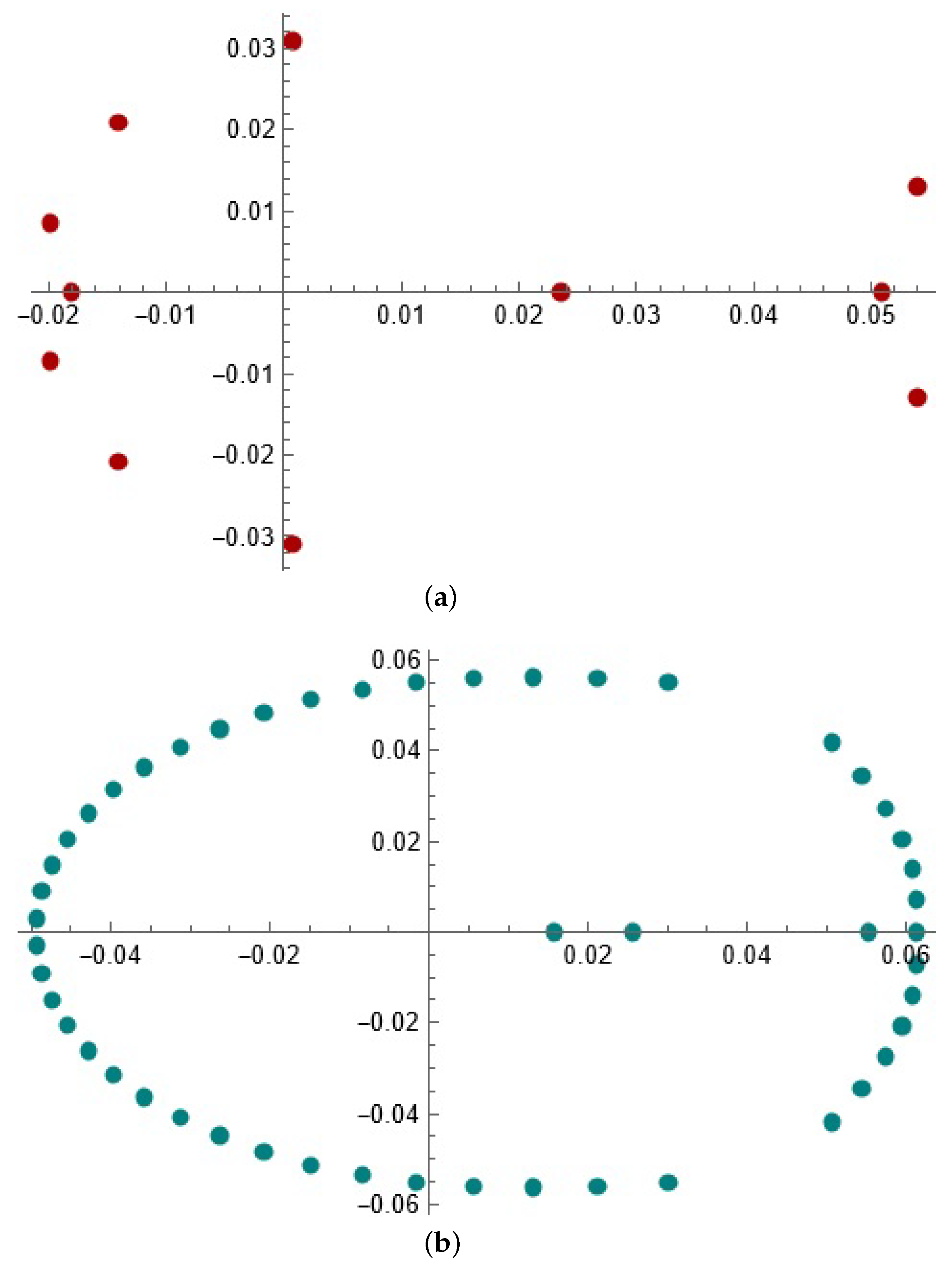
With respect to the study of zeros of the nth Lagrange-based hypergeometric Bernoulli polynomial ${\mathcal{B}}_n^{[m-1,{\alpha }_1,\dots ,{\alpha }_r]}\left(x|x_1,\dots ,x_r\right)$ when $x_1,\dots ,x_r$ are fixed, relatively little is known. For instance, it is possible to use the Hurwitz theorem (see (Chapter I, p. 22)) in [4] for obtaining the fact that the complex zeros of ${\mathcal{B}}_n^{[m-1,{\alpha }_1,\dots ,{\alpha }_r]}\left(x|x_1,\dots ,x_r\right)$ must move further away from the origin as n proceeds to infinity, because the functions to which they converge only have real zeros. In Figure 1, the plots for the zeros of ${\mathcal{B}}_{11}^{[m-1,{\alpha }_1,\dots ,{\alpha }_r]}\left(y\right)$ and ${\mathcal{B}}_{50}^{[m-1,{\alpha }_1,\dots ,{\alpha }_r]}\left(y\right)$ are shown for prescribed values of m and ${\alpha }_1,\dots ,{\alpha }_r$.

There is another relation of Lagrange-based hypergeometric Bernoulli polynomials with Lagrange polynomials and hypergeometric Bernoulli numbers in terms of Stirling numbers of the second kind $S(n,k)$, for which its generating function is given by the following.

$$\frac{{\left(e^z-1\right)}^k}{k!}=\sum _{n=k}^{\infty }S(n,k)\frac{z^n}{n!}.$$

Theorem 2.

For a fixed $m\in \mathbb{N}$ and $n\ge 0$, we have the following.

$${\mathcal{B}}_n^{[m-1,{\alpha }_1,\dots ,{\alpha }_r]}\left(x|x_1,\dots ,x_r\right)=\sum _{j=0}^n\sum _{s=0}^{n-j}\sum _{k=0}^s{g}_j^{\left({\alpha }_1,\dots ,{\alpha }_r\right)}\left(x_1,\dots ,x_r\right)S(n,k)\frac{x^{\left(k\right)}}{s!}\frac{B_{n-s-j}^{[m-1]}}{(n-s-j)!}.$$

(21)

Proof. 

Using (1), (4), and the Abel binomial theorem, we obtain the following.

$$\begin{array}{cc}\hfill \sum _{n=0}^{\infty }{\mathcal{B}}_n^{[m-1,{\alpha }_1,\dots ,{\alpha }_r]}\left(x|x_1,\dots ,x_r\right)z^n& =\left(\prod _{j=1}^r{\left(1-x_{j}z\right)}^{-{\alpha }_j}\right)\left(\sum _{n=0}^{\infty }{B}_n^{[m-1]}\frac{z^n}{n!}\right){\left(\left(e^z-1\right)+1\right)}^x\hfill \\ & =\left(\prod _{j=1}^r{\left(1-x_{j}z\right)}^{-{\alpha }_j}\right)\left(\sum _{n=0}^{\infty }{B}_n^{[m-1]}\frac{z^n}{n!}\right)\left(\sum _{n=0}^{\infty }\left(\genfrac{}{}{0pt}{}{x}{n}\right)n!\sum _{n=k}^{\infty }S(n,k)\frac{z^n}{n!}\right)\hfill \\ & =\left(\prod _{j=1}^r{\left(1-x_{j}z\right)}^{-{\alpha }_j}\right)\left(\sum _{n=0}^{\infty }{B}_n^{[m-1]}\frac{z^n}{n!}\right)\left(\sum _{n=0}^{\infty }\sum _{k=0}^{n}S(n,k)x^{\left(k\right)}\frac{z^n}{n!}\right)\hfill \\ & =\left(\sum _{n=0}^{\infty }\sum _{j=0}^n\sum _{s=0}^{n-j}\sum _{k=0}^s{g}_j^{\left({\alpha }_1,\dots ,{\alpha }_r\right)}\left(x_1,\dots ,x_r\right)S(n,k)\frac{x^{\left(k\right)}}{s!}\frac{B_{n-s-j}^{[m-1]}}{(n-s-j)!}\right)\hfill \end{array}$$

Therefore, comparing the coefficients on both sides, we obtain (21). □

When ${\alpha }_1=\cdots ={\alpha }_r=0$, expression (21) reduces to a relation of hypergeometric Bernoulli polynomials with their numbers in terms of Stirling numbers of the second kind (see, e.g., (Proposition 5)) in [10].

The results in [13,17] allow us to obtain a matrix form of ${\mathcal{B}}_s^{[m-1,{\alpha }_1,\dots ,{\alpha }_r]}\left(x|x_1,\dots ,x_r\right)$, $s=0,1,\dots ,n$, as follows.

Part (a) of Theorem 1 yields the following:

$${\mathcal{B}}_s^{[m-1,{\alpha }_1,\dots ,{\alpha }_r]}\left(x|x_1,\dots ,x_r\right)={\mathbf{G}}_r^{[m-1,{\alpha }_1,\dots ,{\alpha }_r]}(x_1,\dots ,x_r){\mathbf{B}}^{[m-1]}\left(x\right),$$

(22)

where the following is the case:

$${\mathbf{G}}_s^{[m-1,{\alpha }_1,\dots ,{\alpha }_r]}(x_1,\dots ,x_r)=\left[\begin{array}{cccc}{g}_s^{[m-1,{\alpha }_1,\dots ,{\alpha }_r]}(x_1,\dots ,x_r)\cdots & g_0^{[m-1,{\alpha }_1,\dots ,{\alpha }_r]}(x_1,\dots ,x_r)& \cdots & 0\end{array}\right],$$

and the null entries of matrix ${\mathbf{G}}_s^{[m-1,{\alpha }_1,\dots ,{\alpha }_r]}(x_1,\dots ,x_r)$ appear $(n-r)$-times, and the matrix ${\mathbf{B}}^{[m-1]}\left(x\right)$ is given by ${\mathbf{B}}^{[m-1]}\left(x\right)={\left(\begin{array}{cccccc}{B}_0^{[m-1]}\left(x\right)& B_1^{[m-1]}\left(x\right)& \cdots & \frac{B_r^{[m-1]}\left(x\right)}{r!}& \cdots & \frac{B_n^{[m-1]}\left(x\right)}{n!}\end{array}\right)}^T$.

Then, by (22), the matrix of the following:

$${\mathbf{B}}^{[m-1,{\alpha }_1,\dots ,{\alpha }_r]}\left(x|x_1,\dots ,x_r\right)={\left(\begin{array}{ccc}{\mathcal{B}}_0^{[m-1,{\alpha }_1,\dots ,{\alpha }_r]}\left(x|x_1,\dots ,x_r\right)& \cdots & {\mathcal{B}}_n^{[m-1,{\alpha }_1,\dots ,{\alpha }_r]}\left(x|x_1,\dots ,x_r\right)\end{array}\right)}^T,$$

can be expressed as follows:

$$\begin{array}{ccc}\hfill {\mathbf{B}}^{[m-1,{\alpha }_1,\dots ,{\alpha }_r]}\left(x|x_1,\dots ,x_r\right)& =& {\mathbf{G}}^{[m-1,{\alpha }_1,\dots ,{\alpha }_r]}(x_1,\dots ,x_r){\mathbf{B}}^{[m-1]}\left(x\right),\hfill \end{array}$$

(23)

where ${\mathbf{G}}^{[m-1,{\alpha }_1,\dots ,{\alpha }_r]}(x_1,\dots ,x_r)$ is the following $(n+1)\times (n+1)$ matrix.

$${\mathbf{G}}^{[m-1,{\alpha }_1,\dots ,{\alpha }_r]}(x_1,\dots ,x_r)=\left[\begin{array}{cccc}{g}_0^{[m-1,{\alpha }_1,\dots ,{\alpha }_r]}(x_1,\dots ,x_r)& 0& \cdots & 0\\ & & & & \\ g_1^{[m-1,{\alpha }_1,\dots ,{\alpha }_r]}(x_1,\dots ,x_r)& g_0^{[m-1,{\alpha }_1,\dots ,{\alpha }_r]}(x_1,\dots ,x_r)& \cdots & 0\\ & & & & \\ g_2^{[m-1,{\alpha }_1,\dots ,{\alpha }_r]}(x_1,\dots ,x_r)& g_1^{[m-1,{\alpha }_1,\dots ,{\alpha }_r]}(x_1,\dots ,x_r)& \cdots & 0\\ ⋮& ⋮& \ddots & ⋮\\ g_n^{[m-1,{\alpha }_1,\dots ,{\alpha }_r]}(x_1,\dots ,x_r)& g_{n-1}^{[m-1,{\alpha }_1,\dots ,{\alpha }_r]}(x_1,\dots ,x_r)& \cdots & g_0^{[m-1,{\alpha }_1,\dots ,{\alpha }_r]}(x_1,\dots ,x_r)\end{array}\right].$$

The following theorem summarizes the ideas described above.

Theorem 3.

For a fixed $m\in \mathbb{N}$, let ${\left\{{\mathcal{B}}_n^{[m-1,{\alpha }_1,\dots ,{\alpha }_r]}\left(x|x_1,\dots ,x_r\right)\right\}}_{n\ge 0}$ be the sequence of Lagrange-based hypergeometric Bernoulli polynomials in variables $x,x_1,\dots ,x_r$ and parameters ${\alpha }_1,\dots ,{\alpha }_r\in \mathbb{C}$. Then, matrix ${\mathbf{B}}^{[m-1,{\alpha }_1,\dots ,{\alpha }_r]}\left(x|x_1,\dots ,x_r\right)$ has the following matrix form.

$$\begin{array}{c}\hfill {\mathbf{B}}^{[m-1,{\alpha }_1,\dots ,{\alpha }_r]}\left(x|x_1,\dots ,x_r\right)={\mathbf{G}}^{[m-1,{\alpha }_1,\dots ,{\alpha }_r]}(x_1,\dots ,x_r){\mathbf{B}}^{[m-1]}\left(x\right).\end{array}$$

Remark 1.

Note that according to (22), the rows of matrix ${\mathbf{G}}^{[m-1,{\alpha }_1,\dots ,{\alpha }_r]}(x_1,\dots ,x_r)$ are precisely the matrices ${\mathbf{G}}_s^{[m-1,{\alpha }_1,\dots ,{\alpha }_r]}(x_1,\dots ,x_r)$ for $s=0,\dots ,n$. Furthermore, matrix ${\mathbf{G}}^{[m-1,{\alpha }_1,\dots ,{\alpha }_r]}(x_1,\dots ,x_r)$ is an $(n+1)\times (n+1)$ lower triangular matrix for each $x_1,\dots ,x_r\in \mathbb{R}\backslash \left\{0\right\}$ such that the following is the case.

$$det\left({\mathbf{G}}^{[m-1,{\alpha }_1,\dots ,{\alpha }_r]}(x_1,\dots ,x_r)\right)={\left(g_0^{[m-1,{\alpha }_1,\dots ,{\alpha }_r]}(x_1,\dots ,x_r)\right)}^{n+1}=1.$$

Therefore, ${\mathbf{G}}^{[m-1,{\alpha }_1,\dots ,{\alpha }_r]}(x_1,\dots ,x_r)$ is an invertible matrix for each $x_1,\dots ,x_r\in \mathbb{R}\backslash \left\{0\right\}$.

Remark 2.

Using (Equation (8)) in [13], we can deduce the following:

$$\begin{array}{ccc}\hfill {\mathbf{B}}^{[m-1]}\left(x\right)& =& {\mathbf{M}}^{[m-1]}\mathbf{T}\left(x\right)\hfill \\ \hfill & =& \left(\begin{array}{cccccc}\frac{B_0^{[m-1]}}{n!}& 0& 0& 0& \cdots & 0\\ \frac{B_1^{[m-1]}}{(n-1)!}& \frac{B_0^{[m-1]}}{n!}& 0& 0& \cdots & 0\\ \frac{B_2^{[m-1]}}{2!(n-2)!}& \frac{B_1^{[m-1]}}{(n-1)!}& \frac{B_0^{[m-1]}}{n!}& 0& \cdots & 0\\ \frac{B_3^{[m-1]}}{3!(n-3)!}& \frac{B_2^{[m-1]}}{2!(n-2)!}& \frac{B_1^{[m-1]}}{(n-1)!}& \frac{B_0^{[m-1]}}{n!}& \cdots & 0\\ ⋮& ⋮& ⋮& ⋮& \ddots & ⋮\\ \frac{B_n^{[m-1]}}{n!}& \frac{B_{n-1}^{[m-1]}}{(n-1)!}& \frac{B_{n-2}^{[m-1]}}{2!(n-2)!}& \frac{B_{n-3}^{[m-1]}}{3!(n-3)!}& \cdots & \frac{B_0^{[m-1]}}{n!}\end{array}\right)\mathbf{T}\left(x\right),\hfill \end{array}$$

(24)

where $\mathbf{T}\left(x\right)={\left(\begin{array}{cccccc}1& x& \cdots & x^r& \cdots & x^n\end{array}\right)}^T$. Again, matrix ${\mathbf{M}}^{[m-1]}$ is an $(n+1)\times (n+1)$ has a lower triangular matrix satisfying the following.

$$det\left({\mathbf{M}}^{[m-1]}\right)={\left(\frac{B_0^{[m-1]}}{n!}\right)}^{n+1}=\frac{1}{{(n!)}^{n+1}}.$$

Hence, ${\mathbf{M}}^{[m-1]}$ is an invertible matrix.

Finally, on the account of Theorem 3 and Remark 2, we can deduce the following result.

Theorem 4.

For fixed $m\in \mathbb{N}$ and $x_1,\dots ,x_r\in \mathbb{R}\backslash \left\{0\right\}$, let ${\left\{{\mathcal{B}}_n^{[m-1,{\alpha }_1,\dots ,{\alpha }_r]}\left(x|x_1,\dots ,x_r\right)\right\}}_{n\ge 0}$ be the sequence of Lagrange-based hypergeometric Bernoulli polynomials in the variable x, parameters ${\alpha }_1,\dots ,{\alpha }_r\in \mathbb{C}$. Then, the following matrix-inversion formula holds:

$$\begin{array}{c}\hfill \mathbf{T}\left(x\right)={\mathbf{N}}^{[m-1]}{\mathbf{Q}}^{[m-1]}{\mathbf{B}}^{[m-1,{\alpha }_1,\dots ,{\alpha }_r]}\left(x|x_1,\dots ,x_r\right),\end{array}$$

where ${\mathbf{Q}}^{[m-1]}$ and ${\mathbf{N}}^{[m-1]}$ are the inverse matrices of ${\mathbf{G}}^{[m-1,{\alpha }_1,\dots ,{\alpha }_r]}(x_1,\dots ,x_r)$ and ${\mathbf{M}}^{[m-1]}$, respectively.

4. Concluding Remarks

The main goal of our research has been to introduce Lagrange-based hypergeometric Bernoulli polynomials and to investigate some algebraic and analytic properties of these polynomials. We derived summation formulas, differential relations, and integral formulas for them. In addition, an interesting matrix-inversion formula (cf. Theorems 3 and 4) and a generating relation involving the Stirling numbers of the second kind have been derived for these polynomials (see Theorem 2).

In our study, we have obtained some formulas for some classical special numbers and recovered some well-known identities in the literature (Theorems 1 and 2). We have used the techniques of the theory of generating functions, mainly variants of Bernoulli generating functions into our investigation of some new identities for some special numbers. However, there is a different approach for the study of generating functions based on the use of the theory of zeta functions, which provides a new description of special polynomials and special numbers in terms of special values of certain zeta functions such as the Riemann zeta function (cf. [23,24,25] where this approach is adopted). To the best of our knowledge, a unified approach to the study of special numbers remains a work in progress (cf., e.g., [21] or more recently, [22], and references thereof).

We would also like to mention that if we consider the following broad class of generating functions:

$$G(x_1,x_2,\dots ,x_m,z):=\theta \left(z\right)exp\left(-\sum _{k=1}^m{x}_k{z}^k\right),$$

(25)

where $\theta \left(z\right)$ is a function having an explicit Laurent expansion near $z=0$, then (4) becomes a special case of (25).

Hence, some generalizations of this research might be considered probably in the future. Finally, the results of this article might potentially be used in mathematics, in mathematical physics, and/or in engineering.

References

1. Chan, W.-C.C.; Chyan, C.-J.; Srivastava, H.M. The Lagrange polynomials in several variables. Integral Transform. Spec. Funct. 2001, 12, 139–148. [Google Scholar] [CrossRef]
2. Erdélyi, A.; Magnus, W.; Oberhettinger, F.; Tricomi, F. Higher Transcendental Functions; McGraw Hill: New York, NY, USA, 1953; Volume 3, p. 267. [Google Scholar]
3. Mathai, A.M.; Haubold, H.J. Special Functions for Applied Scientists; Springer Science Business Media: New York, NY, USA, 2008; pp. 1–309. [Google Scholar]
4. Szegö, G. Orthogonal Polynomials; American Math. Soc: Providence, RI, USA, 1939; pp. 68–69. [Google Scholar]
5. Srivastava, H.M.; Manocha, H.L. A Treatise on Generating Functions; Ellis Horwood Ltd.: West Sussex, UK, 1984; pp. 378–384, 441–442. [Google Scholar]
6. Bretti, G.; Ricci, P.E. Multidimensional extensions of the Bernoulli and Appell polynomials. Taiwanese J. Math. 2004, 8, 415–428. [Google Scholar] [CrossRef]
7. Bretti, G.; Natalini, P.; Ricci, P.E. Generalizations of the Bernoulli and Appell polynomials. Abstr. Appl. Anal. 2004, 7, 613–623. [Google Scholar] [CrossRef] [Green Version]
8. Natalini, P.; Bernardini, A. A generalization of the Bernoulli polynomials. J. Appl. Math. 2003, 2003, 155–163. [Google Scholar] [CrossRef] [Green Version]
9. Srivastava, H.M.; Özarslan, M.A.; Kaanoğlu, C. Some generalized Lagrange-based Apostol-Bernoulli, Apostol-Euler and Apostol-Genocchi polynomials. Russian J. Math. Phys. 2013, 10, 110–120. [Google Scholar] [CrossRef]
10. Chakraborty, K.; Komatsu, T. Generalized hypergeometric Bernoulli numbers. Rev. R. Acad. Cienc. Exactas Fís. Nat. Ser. A Math. RACSAM 2021, 115, 1–14. [Google Scholar] [CrossRef]
11. Hassen, A.; Nguyen, H.D. Hypergeometric Bernoulli polynomials and Appell sequences. Int. J. Number Theory 2008, 4, 767–774. [Google Scholar] [CrossRef] [Green Version]
12. Howard, F.T. Some sequences of rational numbers related to the exponential function. Duke Math. J. 1967, 34, 701–716. [Google Scholar] [CrossRef]
13. Quintana, Y.; Ramírez, W.; Urieles, A. On an operational matrix method based on generalized Bernoulli polynomials of level m. Calcolo 2018, 55, 1–29. [Google Scholar] [CrossRef]
14. Khan, W.A.; Abouzaid, M.S.; Abusufian, A.H.; Nisar, K.S. Some new classes of generalized Lagrange-based Apostol type Hermite polynomials. J. Inequal. Spec. Funct. 2019, 10, 1–11. [Google Scholar]
15. Khan, W.A. On generalized Lagrange-based Apostol-type and related polynomials. Kragujevac J. Math. 2022, 46, 865–882. [Google Scholar]
16. Duran, U.; Acikgoz, M.; Esi, A.; Araci, S. The Lagrange polynomials in several variables. Appl. Math. Inf. Sci. 2018, 12, 227–231. [Google Scholar] [CrossRef]
17. Quintana, Y. Generalized mixed type Bernoulli-Gegenbauer polynomial. Kragujevac J. Math. 2020, 47, 245–257. [Google Scholar]
18. Cesarano, C.; Ramírez, W.; Khan, S. A new class of degenerate Apostol-type Hermite polynomials and applications. Dolomites Res. Notes Approx. 2022, 15, 1–10. [Google Scholar]
19. Cesarano, C.; Parmentier, A. A note on Hermite-Bernoulli Polynomials. In Nonlocal and Fractional Operators; Beghin, L., Garrappa, R., Mainardi, F., Eds.; Springer Nature: Cham, Switzerland, 2021; Volume 26, pp. 101–109. [Google Scholar]
20. Khan, W.A.; Araci, S.; Acikgoz, M.; Esi, A. Laguerre-based Hermite-Bernoulli polynomials associated with bilateral series. Tbilisi Math. J. 2018, 11, 111–121. [Google Scholar]
21. Hernández-Llanos, P.; Quintana, Y.; Urieles, A. About extensions of generalized Apostol-type polynomials. Results Math. 2015, 68, 203–225. [Google Scholar] [CrossRef]
22. Navas, L.; Ruiz, F.J.; Varona, J.L.; Bernardini, A. Existence and reduction of generalized Apostol-Bernoulli, Apostol-Euler and Apostol-Genocchi polynomials. Arch. Math. 2019, 55, 157–165. [Google Scholar]
23. Bayad, A. Special values of Lerch zeta function and their Fourier expansions. Adv. Stud. Contemp. Math. 2011, 21, 1–4. [Google Scholar]
24. Bayad, A.; Hajli, M. On the multidimensional zeta functions associated with theta functions, and the multidimensional Appell polynomials. Math. Methods Appl. Sci. 2020, 43, 2679–2694. [Google Scholar] [CrossRef]
25. Hajli, M. On a formula for the regularized determinant of zeta functions with application to some Dirichlet series. Q. J. Math. 2020, 71, 843–865. [Google Scholar] [CrossRef]
Figure 1. Plot for the zeros of B 11 [ m 1 , α 1 , α 2 , α 3 , α 4 ] ( y ) (a) and plot for the zeros of B 50 [ m 1 , α 1 , , α r ] ( y ) (b), when m = 6 and α 1 = 1 / 4 , α 2 = 1 , α 3 = 2 , α 4 = 3 .
Symmetry 14 01125 g001
Publisher’s Note: MDPI stays neutral with regard to jurisdictional claims in published maps and institutional affiliations.