Double Roman Domination in Generalized Petersen Graphs P(ck, k)

Abstract

A double Roman dominating function on a graph $G=(V,E)$ is a function $f:V\to \{0,1,2,3\}$, satisfying the condition that every vertex u for which $f\left(u\right)=1$ is adjacent to at least one vertex assigned 2 or 3, and every vertex u with $f\left(u\right)=0$ is adjacent to at least one vertex assigned 3 or at least two vertices assigned 2. The weight of f equals the sum $w\left(f\right)={\sum }_{v\in V}f\left(v\right)$. The minimum weight of a double Roman dominating function of G is called the double Roman domination number ${\gamma }_{dR}\left(G\right)$ of a graph G. We obtain tight bounds and in some cases closed expressions for the double Roman domination number of generalized Petersen graphs $P(ck,k)$. In short, we prove that ${\gamma }_{dR}\left(P(ck,k)\right)=\frac{3}{2}ck+\epsilon$, where ${\displaystyle \underset{c\to \infty ,k\to \infty }{lim}\frac{\epsilon }{ck}=0}$.

1. Introduction

Double Roman domination of graphs [1] is motivated by many applications at the present time and in the past [2]. Initially, modern studies of Roman domination [3,4] were inspired by a real problem from the 4th century, when the Old Roman Emperor Constantine was faced with a problem of how to defend his empire with a limited number of armies. The decision was taken to allocate two types of military units to the empire provinces. Some units were able to move quickly from one province to another to respond to any attack. The second type were the local militia. These armies were permanently positioned in their home province. Emperor Constantine ordered that no legion should ever leave the province to defend the second, if in this case the first province remains undefended. Consequently, there were two armies at some provinces, and at some other provinces only local militia units were stationed. Some provinces had no permanent presence of an army, and were guarded by the armies from neighbouring provinces. Although the classical problem is still of interest in military operations research [5], it also can be used to model and solve the problems where a time-critical service needs to be provided with some reserve. For example, a first aid emergency station should never send all its crew to answer an emergency call.

Following the reasoning above, understanding the double Roman domination problem and its variants may be crucial for positioning the fire stations, first aid stations, etc. at optimal positions. This may greatly improve the public services at no extra cost. A natural generalization of double Roman domination is the k-Roman domination [6]. In case of emergency services, k teams are planned to be quickly available in case of severe emergency calls. The special case, $k=2$, is called double Roman domination.

The decision version of the double Roman domination problem (MIN-DOUBLE-RDF) is known to be NP-complete, also in cases when we are restricted to some special classes of graphs, for example, to planar graphs, bipartite graphs, chordal (bipartite) graphs, circle graphs, and to undirected path graphs [7,8,9]. Due to the intractability of the problem, several avenues of research are of interest. For example, studies of the complexity of the problem for special families of graphs has been performed in the past. The results include linear time algorithms for interval graphs and block graphs [8], for trees [10], for proper interval graphs [11], and for unicyclic graphs [9]. Another popular way to explore are attempts to find closed expressions for the double Roman domination number of some graph families. Among popular examples are generalized Petersen graphs and some of their subfamilies that have been extensively studied recently. The published results include (see the subsection on related previous work) closed expressions for the double Roman domination number of some, and tight bounds for other subfamilies [12,13,14,15]. For more related work, we refer to [16,17,18,19] and the references there.

Here, in Section 2.4, we summarize the previously known results on double Roman domination of generalized Petersen graphs $P(ck,k)$ for $c=3,4,5$ and provide improved new general bounds for arbitrary c. The rest of the paper is organized as follows. In Section 2 we summarize some basic definitions and previous results which are used in the following sections. In particular, our main result is outlined in Section 2.5. The constructions and proofs are in Section 3, Section 4, Section 5 and Section 6. In the last section, we discuss the asymptotics and compare the new bounds to the best previously known.

2. Preliminaries

The definitions in the following subsections are recalled from [20].

2.1. Graphs and Double Roman Domination

Assume $G=(V,E)$ is a graph without loops and multiple edges. Let $V=V\left(G\right)$ be the vertex set of G and $E=E\left(G\right)$ its edge set. A set $D\subseteq V\left(G\right)$ is called a dominating set of G if every vertex in $V\left(G\right)\backslash D$ has at least one neighbour in D. The cardinality of a minimum dominating set of G is called the domination number $\gamma \left(G\right)$. A double Roman dominating function (DRDF) on a graph $G=(V,E)$ is a function $f:V\to \{0,1,2,3\}$ with the properties that

(1)

every vertex u with $f\left(u\right)=0$ is adjacent to at least one vertex assigned 3 or at least two vertices assigned 2, and

(2)

every vertex u with $f\left(u\right)=1$ is adjacent to at least one vertex assigned 2 or 3.

For an arbitrary subset $U\subseteq V\left(G\right)$ define the weight of f on U as $w\left(f\left(U\right)\right)={\sum }_{u\in U}f\left(u\right)$. Then, the weight of f equals $w\left(f\right)=w\left(f\left(G\right)\right)={\sum }_{v\in V\left(G\right)}f\left(v\right)$. The double Roman domination number ${\gamma }_{dR}\left(G\right)$ of a graph G is the minimum weight of a double Roman dominating function of G. A DRD function f is called a ${\gamma }_{dR}$-function of G if $w\left(f\right)={\gamma }_{dR}\left(G\right)$.

Let f be a double Roman dominating function on G. We define the corresponding double Roman dominating partition $(D_0,D_1,D_2,D_3)$ of the vertex set $V=D_0\cup D_1\cup D_2\cup D_3$, where $D_i=D_i^f=\left\{u\right|f\left(u\right)=i\}$.

The study of the double Roman domination in graphs was initiated by Beeler et al. [1]. It was proved that $2\gamma \left(G\right)\le {\gamma }_{dR}\left(G\right)\le 3\gamma \left(G\right)$, and observed that in a double Roman dominating function f of weight ${\gamma }_{dR}\left(G\right)$, no vertex needs to be assigned the value 1.

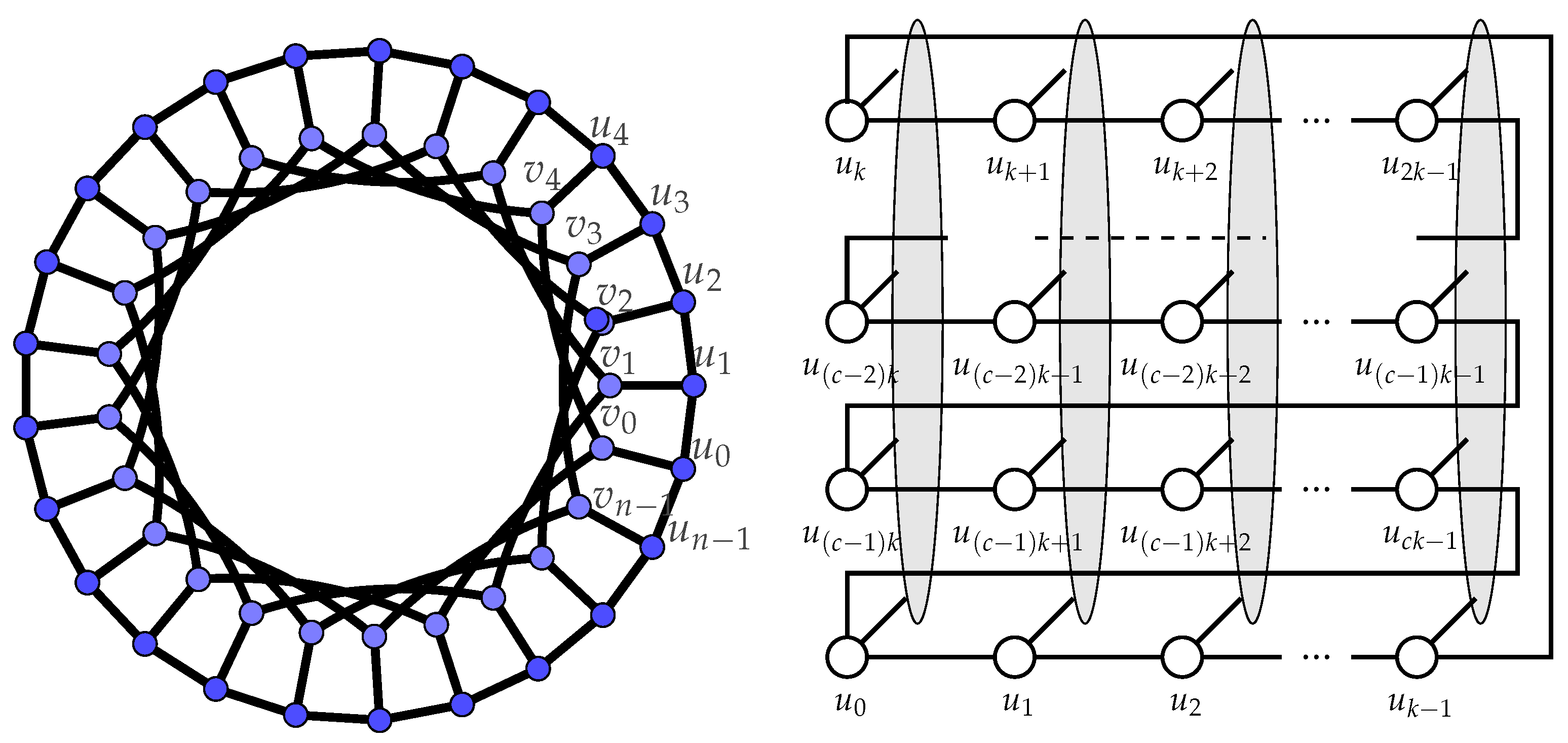
2.2. Generalized Petersen Graphs

The generalized Petersen graph $P(n,k)$ is a graph with vertex set $U\cup V$ and edge set $E_1\cup E_2\cup E_3$, where $U=\{u_0,u_1,\dots ,u_{n-1}\}$, $V=\{v_0,v_1,\cdots ,v_{n-1}\}$, $E_1=\left\{u_i{u}_{i+1}\right|i=0,1,\dots ,n-1\}$, $E_2=\left\{u_i{v}_i\right|i=0,1,\dots ,n-1\}$, $E_3=\left\{v_i{v}_{i+k}\right|i=0,1,\dots ,n-1\}$. All subscripts are reduced modulo n (see Figure 1). Thus we identify integers i and j iff $i\equiv jmodn$.

It is well known that the graphs $P(n,k)$ are 3-regular unless $k=\frac{n}{2}$ and that $P(n,k)$ are highly symmetric [21,22]. As $P(n,k)$ and $P(n,n-k)$ are isomorphic, it is natural to restrict attention to $P(n,k)$ with $n\ge 3$ and k, $1\le k<\frac{n}{2}$.

In this paper, we study generalized Petersen graphs for which $n=ck$. In this case, the graph $P(ck,k)$ has, in addition to the long outer cycle, k shorter cycles of length c, called the inner cycles (see Figure 1, right). For graphs $P(ck,k)$, we will also use the following notation. We denote

$$\begin{array}{ccc}\hfill V_i& =& \{v_{ik},v_{ik+1},v_{ik+2},\cdots ,v_{ik+k-1}\},i=0,1,\cdots ,c-1,\hfill \\ \hfill U_i& =& \{u_{ik},u_{ik+1},u_{ik+2},\cdots ,u_{ik+k-1}\},i=0,1,\cdots ,c-1,\hfill \\ \hfill V& =& {\displaystyle \bigcup _{i=0}^{c-1}{V}_i,U=\bigcup _{i=0}^{c-1}{U}_i,}V\left(P(ck,k)\right)=V\cup U.\hfill \end{array}$$

Observe that each of the sets $V_i$ meets all the inner cycles, and vertices of $U_i$ are exactly the neighbors of $V_i$ on the outer cycle.

Petersen graphs are among the most interesting examples when considering nontrivial graph invariants [23]. In particular, the domination and its variations, such as Roman domination and double Roman domination have been extensively studied in the last years.

2.3. Graph Covers

Following the approach used in [24], we will summarize the basic definition of a covering graph. Let $G=(V_1,E_1)$ and $H=(V_2,E_2)$ be two graphs, and let $p:V_2\to V_1$ be a surjection. We say p is a covering map from H to G if for each $v\in V_2$, the restriction of p to the neighbourhood of $v\in V_2$ is a bijection onto the neighbourhood of $p\left(v\right)$ in G. In other words, p maps edges incidental to v one-to-one onto edges incidental to $p\left(v\right)$. If there exists a covering map from H to G, we will call H a covering graph, or a lift, of G. H is called an h-lift of G if p has a property that for every vertex $v\in V\left(G\right)$, its fiber $p^{-1}\left(v\right)$ has exactly h elements. For some more information on covering graphs see [25].

Obviously, a long cycle can be a covering graph of shorter cycles. For example, the cycle $C_{120}$ is a 2-lift of $C_{60}$, using the surjection $p\left(v_i\right)=v_{imod60}$. Furthermore, $C_{120}$ is also a 30-lift of $C_4$, etc.

2.4. Related Previous Work

To ensure better transparency, we have gathered most of the important results of the previous work in the following

Table 1. Previously known results on domination number of generalized Petersen graphs $P(n,k)$.

Results	References
$k\ge 1$, $c\ge 3$:
$\gamma \left(P(ck,k)\right)\le \left\{\begin{array}{cc}\frac{c}{3}⌈\frac{5k}{3}⌉,\hfill & c\equiv 0mod3,\hfill \\ ⌈\frac{c}{3}⌉⌈\frac{5k}{3}⌉-⌈\frac{2k}{3}⌉,\hfill & c\equiv 1mod3,\hfill \\ ⌈\frac{c}{3}⌉⌈\frac{5k}{3}⌉-⌈\frac{2k}{3}⌉+⌈\frac{k}{3}⌉,\hfill & c\equiv 2mod3.\hfill \end{array}\right.$	Zhao et al. [26]
$\gamma \left(P(4k,k)\right)=\left\{\begin{array}{cc}2k;\hfill & k\equiv 1mod2,\hfill \\ 2k+1;\hfill & k\equiv 0mod2\hfill \end{array}\right.$
$\gamma \left(P\right(5k,k\left)\right)=3k$ for all $k\ge 1$.	Wang et al. [27]

,

Table 2. Previously known results on double Roman domination number of generalized Petersen graphs $P(n,k)$.

Results	References
$n\ge 3$:
${\gamma }_{dR}\left(P(n,1)\right)=\left\{\begin{array}{cc}\frac{3n}{2},\hfill & n\equiv 0mod4,\hfill \\ \frac{3n+3}{2},\hfill & n\equiv 1,3mod4,\hfill \\ \frac{3n+4}{2},\hfill & n\equiv 2mod4\hfill \end{array}\right.$	Shao et al. [13]
$n\ge 5$:
${\gamma }_{dR}\left(P(n,2)\right)=\left\{\begin{array}{cc}⌈\frac{8n}{5}⌉,\hfill & n\equiv 0mod5,\hfill \\ ⌈\frac{8n}{5}⌉+1,\hfill & n\equiv 1,2,3,4mod5.\hfill \end{array}\right.$	Jiang et al. [15]
If G is a graph of maximum degree $▵\ge 1$: ${\gamma }_{dR}\left(G\right)\ge ⌈\frac{3\left|V\right(G\left)\right|}{▵+1}⌉.$
${\gamma }_{dR}\left(P(n,k)\right)\ge \lceil \frac{3n}{2}\rceil .$	Shao et al. [13]
$k\ge 3$:    ${\gamma }_{dR}\left(P(n,k)\right)=\frac{3n}{2}$, $k\equiv 1mod2,n\equiv 0mod4.$
${\gamma }_{dR}\left(P(n,k)\right)\le \left\{\begin{array}{cc}\frac{3n}{2}+\frac{5k+5}{4},\hfill & k\equiv 1mod4,n\not\equiv 0mod4,\hfill \\ \frac{3n}{2}+\frac{5k+7}{4},\hfill & k\equiv 3mod4,n\not\equiv 0mod4,\hfill \\ \frac{3n}{2}\frac{(3k+2)}{(3k+1)},\hfill & k\equiv 0mod4,\hfill \\ & n\equiv 0mod(3k+1),\hfill \\ \lceil \frac{3n}{2}\frac{(3k+2)}{(3k+1)}\rceil +\frac{5k+4}{4},\hfill & k\equiv 0mod4,\hfill \\ & n\not\equiv 0mod(3k+1),\hfill \\ \frac{3n}{2}\frac{\left(3k\right)}{(3k-1)},\hfill & k\equiv 2mod4,\hfill \\ & n\equiv 0mod(3k-1),\hfill \\ \lceil \frac{3n}{2}\frac{\left(3k\right)}{(3k-1)}\rceil +\frac{5k+6}{4},\hfill & k\equiv 2mod4,\hfill \\ & n\not\equiv 0mod(3k-1).\hfill \end{array}\right.$	Gao et al. [12]

and

Table 3. Previously known results on double Roman domination number of generalized Petersen graphs $P(ck,k)$ for small c.

Results	References
${\gamma }_{dR}\left(P(3k,k)\right)=\left\{\begin{array}{cc}5k+1,\hfill & k\in \{1,2,4\}\hfill \\ 5k,\hfill & \mathrm{otherwise}\hfill \end{array}\right.$	Shao et al. [14]
${\gamma }_{dR}\left(P(4,1)\right)=6$, ${\gamma }_{dR}\left(P(8,2)\right)=14$, ${\gamma }_{dR}\left(P(10,2)\right)=16$	Jiang et al. [15]
${\gamma }_{dR}\left(P(12,3)\right)=18$, ${\gamma }_{dR}\left(P(5,1)\right)=9$	Shao et al. [13]
${\gamma }_{dR}\left(P(4k,k)\right)=\left\{\begin{array}{cc}6k,\hfill & k\mathrm{odd}\hfill \\ 6k+3,\hfill & k>2\mathrm{even}\hfill \end{array}\right.$	Folklore, C.F. [20]
$23\le {\gamma }_{dR}\left(P(15,3)\right)\le 26$	Gao et al. [12]
$k\ge 2$:
$8k\le {\gamma }_{dR}\left(P(5k,k)\right)\le \left\{\begin{array}{cc}8k,\hfill & k\equiv 2,3mod5\hfill \\ 8k+2,\hfill & \mathrm{otherwise}\hfill \end{array}\right.$	Rupnik P. et al. [20]

.

The double Roman domination number on Petersen graphs $P(ck,k)$ for small c ($c=3$, 4 and 5) has been studied in recent years. The results are summarized in Table 3.

In [20], it has been proven that certain generalized Petersen graphs are covering graphs of some other generalized Petersen graphs.

Proposition 1

([20]). Let $k\ge 1$, $c_0\ge 3$, and $h\ge 2$. The generalized Petersen graph $P(\left(h{c}_0\right)k,k)$ is an h-lift of $P(c_{0}k,k)$.

Proposition 1 immediately provides a method for establishing upper bounds for double Roman domination numbers of h-lifts.

Proposition 2

([20]). ${\gamma }_{dR}\left(P(\left(h{c}_0\right)k,k)\right)\le h{\gamma }_{dR}\left(P(c_{0}k,k)\right)$.

2.5. Our Results

The main results of this paper are either exact values or narrow bounds for the double Roman domination numbers of all Petersen graphs $P(ck,k)$, $c\ge 3$, $k\ge 3$.

More precisely, we will prove the following theorem.

Theorem 1.

Let $c\ge 3$, and $k\ge 3$.

• If $c\equiv 0mod4$ and k odd, then

  $${\gamma }_{dR}\left(P(ck,k)\right)=\frac{3}{2}ck.$$
• If $c\not\equiv 0mod4$ and k odd, then

  $$\frac{3}{2}ck\le {\gamma }_{dR}\left(P(ck,k)\right)<\left\{\begin{array}{cc}\frac{3}{2}(c+\frac{1}{2})k,\hfill & c\equiv 1,3mod4,\hfill \\ \frac{3}{2}(c+\frac{2}{3})k,\hfill & c\equiv 2mod4,\hfill \end{array}.\right.$$
• For k even, it holds

  $$\frac{3}{2}ck\le {\gamma }_{dR}\left(P(ck,k)\right)<\left\{\begin{array}{cc}\frac{3}{2}c(k+\frac{1}{2}),\hfill & c\equiv 0mod4,\hfill \\ \frac{3}{2}(c+\frac{1}{2})(k+\frac{1}{2}),\hfill & c\equiv 1,3mod4,\hfill \\ \frac{3}{2}(c+\frac{2}{3})(k+\frac{1}{2}),\hfill & c\equiv 2mod4,\hfill \end{array}.\right.$$

3. Constructions and Proofs—Overview

Below we first observe that applying Propositions 1 and 2 gives exact values of double Roman domination number for all $P(ck,k)$ where $c\equiv 0mod4$ and k odd.

The second tool is provided by two constructions that transform $P(ck,k)$ to $P\left(\right(c-1)k,k)$ and $P(ck,k)$ to $P\left(c\right(k-1),k-1)$ by deleting some vertices and adding some edges. It is shown in Propositions 3 and 4 that the result of the construction indeed is isomorphic to $P\left(\right(c-1)k,k)$ and to $P\left(c\right(k-1),k-1)$. Based on the first construction, the upper bounds for ${\gamma }_{dR}\left(P(ck,k)\right)$ are established for arbitrary c by using exact values for ${\gamma }_{dR}\left(P(ck,k)\right)$, where $h=\lceil \frac{c}{4}\rceil$ and k odd (see Section 5). The second construction allows extension of the results to even k (elaborated upon in Section 6).

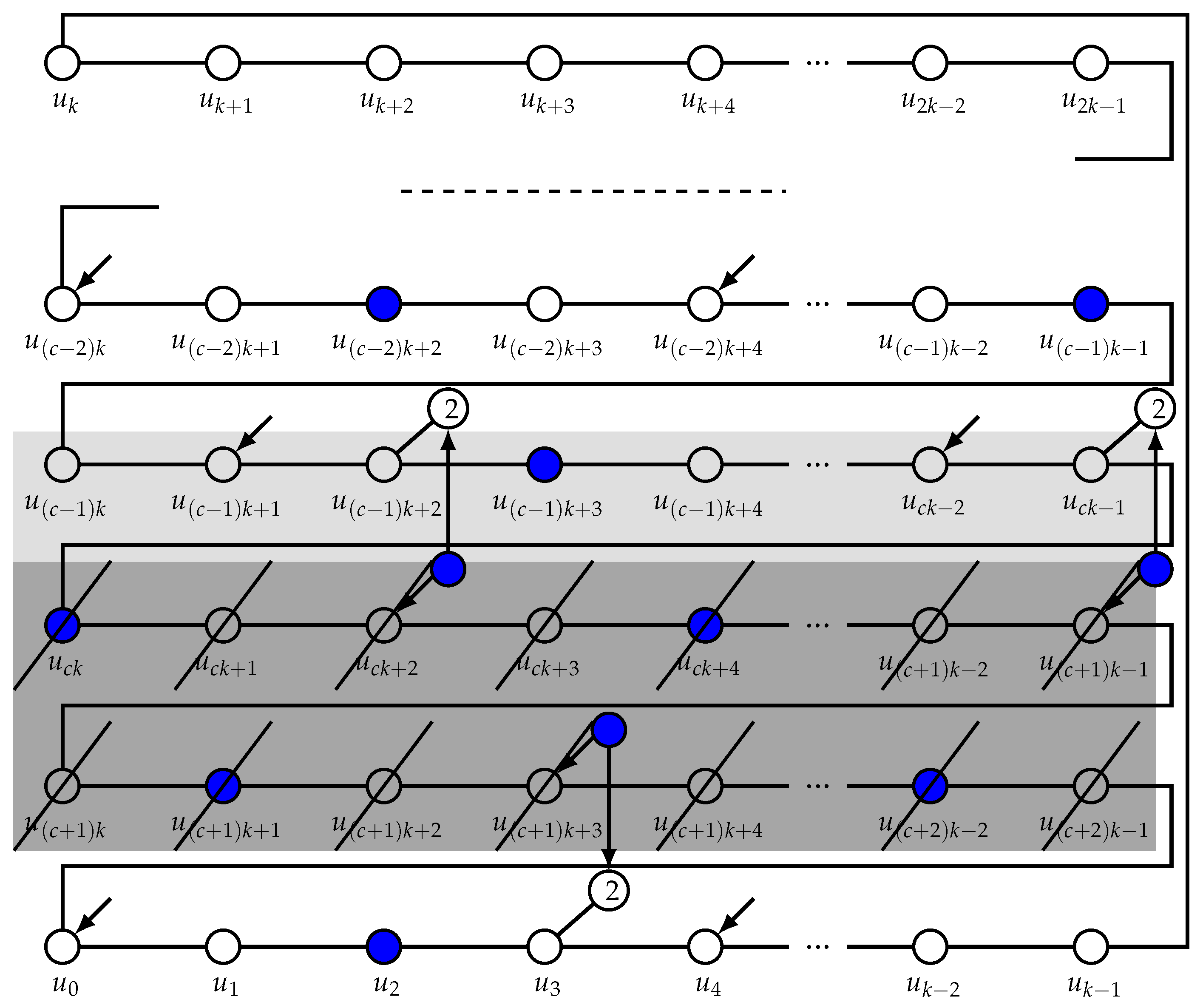
4. The Constructions

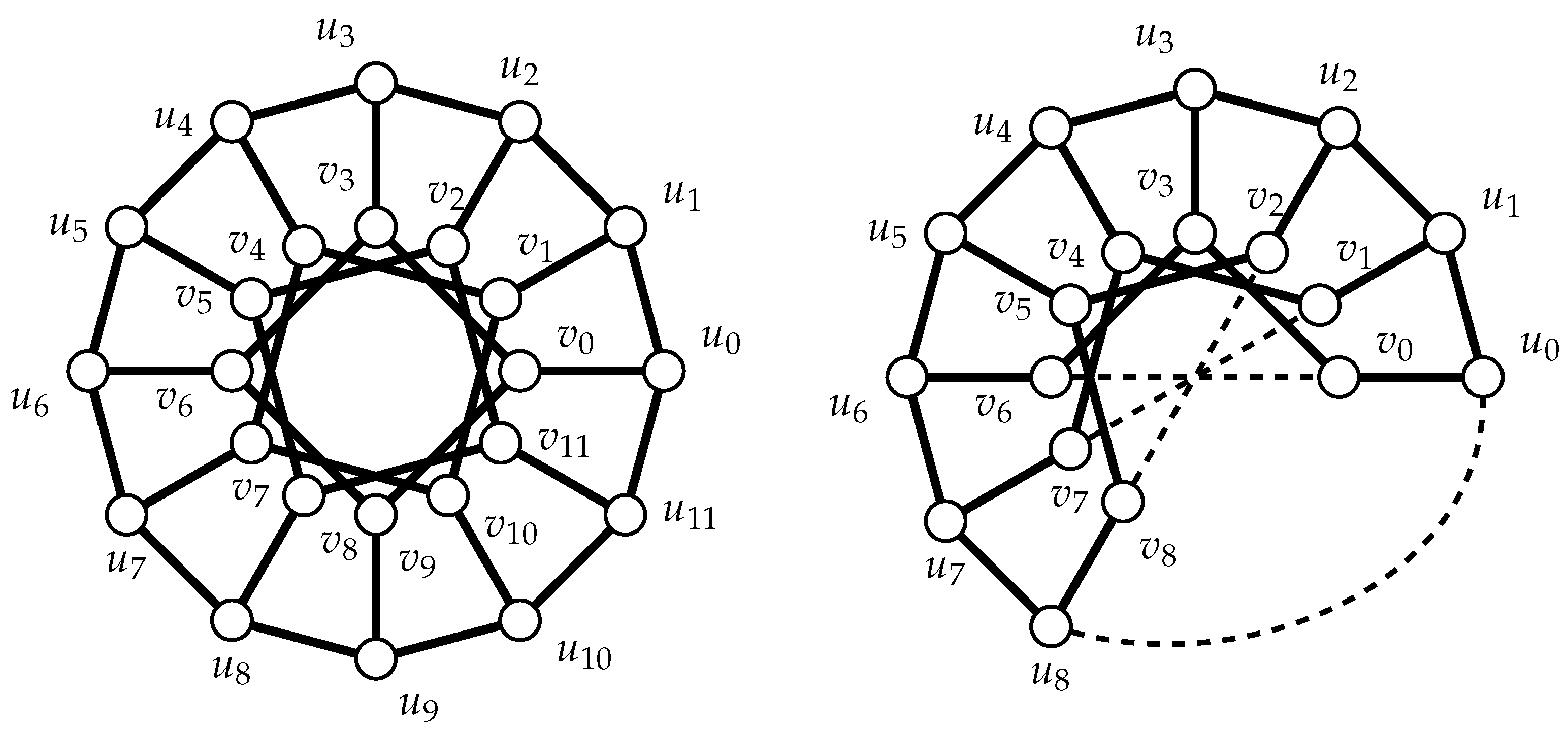
In the continuation we will heavily use the following construction which produces the graph $P\left(\right(c-1)k,k)$ from $P(ck,k)$.

Construction 1.

• Start with$P(ck,k)$.
• Delete vertices
  $V_{c-1}=\{v_{(c-1)k},v_{(c-1)k+1},v_{(c-1)k+2},\cdots ,v_{ck-1}\}$and
  $U_{c-1}=\{u_{(c-1)k},u_{(c-1)k+1},u_{(c-1)k+2},\cdots ,u_{ck-1}\}$
  and delete all edges incident to these vertices.
• Add edges$\{v_{(c-2)k}{v}_0,v_{(c-2)k+1}{v}_1,v_{(c-2)k+2}{v}_2,\cdots v_{(c-1)k-1}{v}_{k-1}\}$on the inner cycles and edge$\left\{u_{(c-1)k-1}{u}_0\right\}$on the outer cycle.

The construction is illustrated on example, from $P(12,3)$ to $P(9,3)$ (see Figure 2).

Proposition 3.

Construction Section 4 on $P(ck,k)$ results in the graph $P\left(\right(c-1)k,k)$.

Proof. 

Obviously, by the construction, each last vertex of each inner cycle is deleted, together with its neighbor on the outer cycle. The labels of the remaining vertices are the same as the standard labeling of $P\left(\right(c-1)k,k)$, and it is easy to see that the construction adds exactly the edges that are missing to obtain $P\left(\right(c-1)k,k)$. □

Obviously, repeated construction results in graphs $P\left(\right(c-2)k,k)$ and $P\left(\right(c-3)k,k)$.

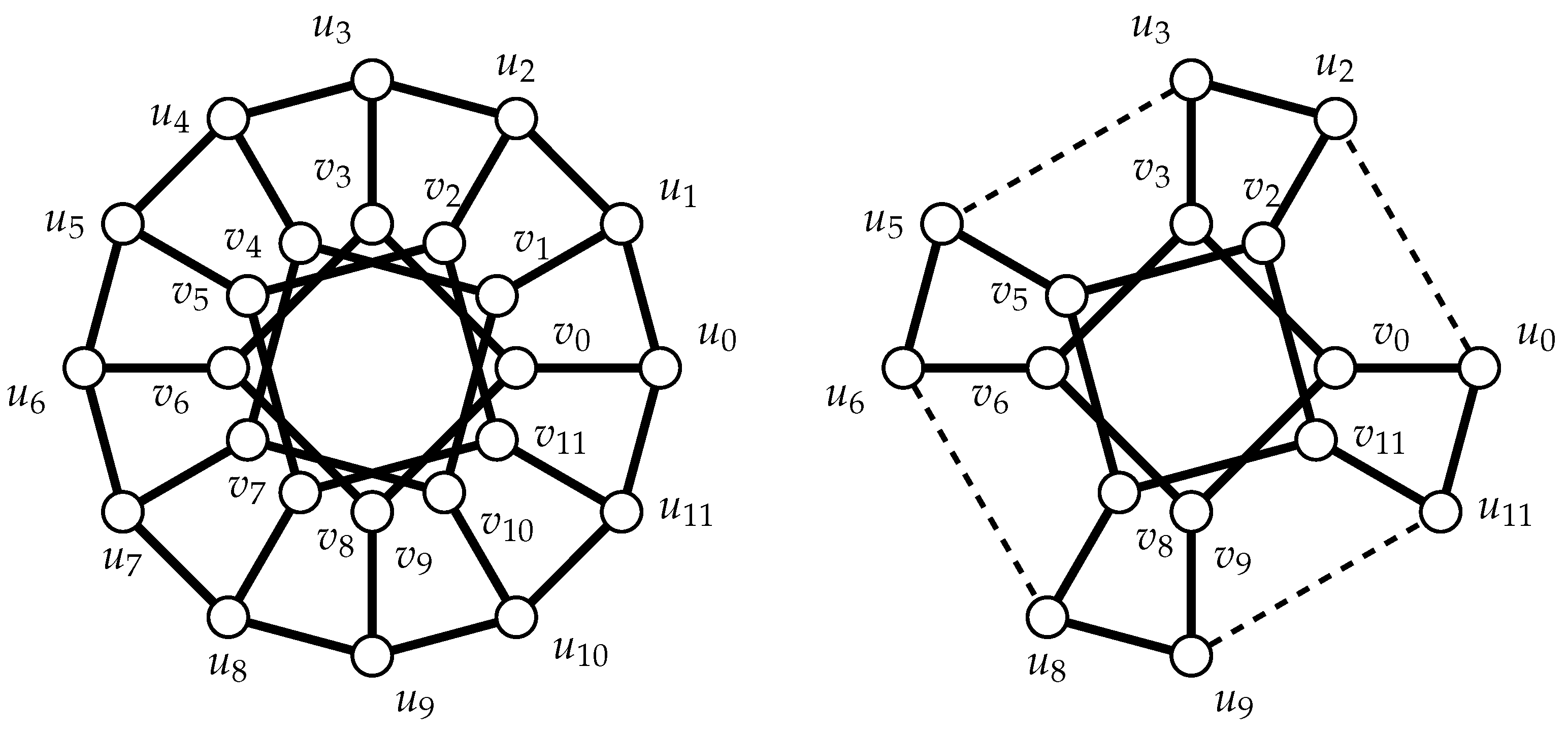
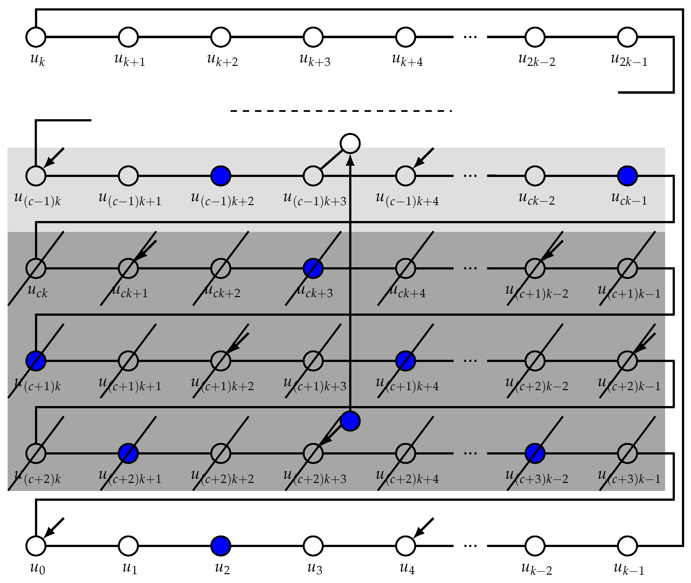
The second construction transforms $P(ck,k)$ to $P\left(c\right(k-1),k-1)$.

Construction 2.

• Start with$P(ck,k)$. Choose$K\in \{0,1,\dots ,k-1\}$.
• Delete the vertices$Ou{t}_K=\left\{u_{jk+K}\right|j=0,1,2,\dots ,c-1\}$and vertices of the corresponding inner cycle$In{n}_K=\left\{v_{jk+K}\right|j=0,1,2,\dots ,c-1\}$and delete all edges incident to these vertices.
• Add edges$u_{jk+K-1}{u}_{jk+K+1}$ for $j=0,1,2,\dots ,c-1$.

The construction is illustrated on example, from $P(12,3)$ to $P(8,2)$ (see Figure 3).

Proposition 4.

Construction Section 4 on $P(ck,k)$ results in the graph that is isomorphic to $P\left(c\right(k-1),k-1)$.

Proof. 

(Sketch.) Recall that the Petersen graph $P(ck,k)$ consists of a long outer cycle and k inner cycles of length c.

Let us choose one inner cycle and delete its vertices and all edges incident to these vertices. The resulting graph has exactly c vertices of degree 2 on the outer cycle. Deleting these vertices and replacing each of the paths of length two with a new edge clearly results in a graph that has $k-1$ cycles of length c, and one long (outer cycle of length $ck-k=c(k-1)$. Observe that this graph is isomorphic to $P\left(c\right(k-1),k-1)$. We omit obvious technical details. □

We continue with explicit constructions of double Roman dominating sets that directly imply upper bounds, and, in some cases, exact values of $P(ck,k)$.

5. Odd k

Recall that for odd k, exact values of double Roman domination number are known, namely (see Table 3)

$${\gamma }_{dR}\left(P(4k,k)\right)=6k.$$

(1)

In this section we first generalize this result to obtain exact values of ${\gamma }_{dR}\left(P(ck,k)\right)$ for $c=4h$ (or, $c\equiv 0mod4$). Then we consider the cases where $c\not\equiv 0mod4$, and provide double Roman dominating functions implying upper bounds in each case.

5.1. Case $c\equiv$ 0 mod 4

Proposition 5.

Let $k\ge 1$ and $c=4h$.

If $k\equiv 1mod2$, then ${\gamma }_{dR}\left(P(ck,k)\right)={\gamma }_{dR}\left(P(4hk,k)\right)=h{\gamma }_{dR}\left(P(4k,k)\right)=6hk=\frac{3}{2}ck$.

Proof. 

Let $c=4h$. Then, Propositions 1 and 2 imply

• $P\left(\right(h4)k,k)$ is a h-lift of $P(4k,k)$ and, consequently,
• ${\gamma }_{dR}\left(P(\left(h4\right)k,k)\right)\le h{\gamma }_{dR}\left(P(4k,k)\right)=6hk$.

Recalling the general lower bound ([13], see Table 3) we conclude that the statement holds. □

For later use, observe that application of Proposition 1 provides explicit construction of the double Roman dominating partition. More precisely, for example,

$$\begin{array}{ccc}\hfill D_3& =& \left\{v_{0+4i}\right|i=0,1,\dots ,k-1\}\cup \left\{u_{2+4i}\right|i=0,1,\dots ,k-1\}\hfill \\ \hfill D& =& (\varnothing ,\varnothing ,\varnothing ,D_3)\hfill \end{array}$$

(2)

is a double Roman domination partition for $P(4k,k)$ of minimal weight. We call this partition the basic double Roman domination partition of $P(4k,k)$. Let f be the corresponding double Roman dominating function. Then $f\left(x\right)=3$ for $x\in D_3$ and $f\left(x\right)=0$ otherwise.

Looking more closely to the partition, if $k=4\ell +3$, then by trivial counting we observe that

$$\begin{array}{c}\hfill \begin{array}{ccc}w\left(f\left(U_{c-4}\right)\right)\hfill & =\hfill & 3(\ell +1),w\left(f\left(V_{c-4}\right)\right)=3(\ell +1),\hfill \\ w\left(f\left(U_{c-3}\right)\right)\hfill & =\hfill & 3\ell ,w\left(f\left(V_{c-3}\right)\right)=3(\ell +1),\hfill \\ w\left(f\left(U_{c-2}\right)\right)\hfill & =\hfill & 3(\ell +1),w\left(f\left(V_{c-2}\right)\right)=3(\ell +1),\hfill \\ w\left(f\left(U_{c-1}\right)\right)\hfill & =\hfill & 3(\ell +1),w\left(f\left(V_{c-1}\right)\right)=3\ell .\hfill \end{array}\end{array}$$

(3)

In fact,

$$\begin{array}{c}\hfill \begin{array}{ccc}\mathrm{if}i\equiv 0mod4\mathrm{then}w\left(f\left(U_i\right)\right)\hfill & =\hfill & 3(\ell +1),w\left(f\left(V_i\right)\right)=3(\ell +1),\hfill \\ \mathrm{if}i\equiv 1mod4\mathrm{then}w\left(f\left(U_i\right)\right)\hfill & =\hfill & 3\ell ,w\left(f\left(V_i\right)\right)=3(\ell +1),\hfill \\ \mathrm{if}i\equiv 2mod4\mathrm{then}w\left(f\left(U_i\right)\right)\hfill & =\hfill & 3(\ell +1),w\left(f\left(V_i\right)\right)=3(\ell +1),\hfill \\ \mathrm{if}i\equiv 3mod4\mathrm{then}w\left(f\left(U_i\right)\right)\hfill & =\hfill & 3(\ell +1),w\left(f\left(V_i\right)\right)=3\ell .\hfill \end{array}\end{array}$$

(4)

It is useful to observe that summing up the weight of the sets for any two consecutive indices gives $3k$, i.e.,

$$w\left(f\left(U_{i-1}\right)\right)+w\left(f\left(V_{i-1}\right)\right)+w\left(f\left(U_i\right)\right)+w\left(f\left(V_i\right)\right)=3(4\ell +3)=3k.$$

(5)

Also note that in the case $k=4\ell +1$, by similar reasoning, we have

$$\begin{array}{c}\hfill \begin{array}{ccc}w\left(f\left(U_{c-4}\right)\right)\hfill & =\hfill & 3\ell ,w\left(f\left(V_{c-4}\right)\right)=3(\ell +1),\hfill \\ w\left(f\left(U_{c-3}\right)\right)\hfill & =\hfill & 3\ell ,w\left(f\left(V_{c-3}\right)\right)=3\ell ,\hfill \\ w\left(f\left(U_{c-2}\right)\right)\hfill & =\hfill & 3(\ell +1),w\left(f\left(V_{c-2}\right)\right)=3\ell ,\hfill \\ w\left(f\left(U_{c-1}\right)\right)\hfill & =\hfill & 3\ell ,w\left(f\left(V_{c-1}\right)\right)=3\ell .\hfill \end{array}\end{array}$$

(6)

and, again, $w\left(f\left(U_{i-1}\right)\right)+w\left(f\left(V_{i-1}\right)\right)+w\left(f\left(U_i\right)\right)+w\left(f\left(V_i\right)\right)=3(4\ell +1)=3k,$ for all i.

Let us summarize the observations for a later reference formally.

Proposition 6.

Let $c\equiv 0mod4$ and k odd. Then the basic double Roman dominating partition of $V\left(P\right(ck,k\left)\right)$:

$$\begin{array}{ccc}\hfill D_3& =& \left\{v_{0+4i}\right|i=0,1,\dots ,k-1\}\cup \left\{u_{2+4i}\right|i=0,1,\dots ,k-1\}\hfill \\ \hfill D& =& (\varnothing ,\varnothing ,\varnothing ,D_3)\hfill \end{array}$$

(7)

gives rise to a double Roman domination function f that is a ${\gamma }_{dR}$-function. Furthermore, for the function f, it holds that

$$w\left(f\left(U_{c-1}\right)\right)+w\left(f\left(V_{c-1}\right)\right)+w\left(f\left(U_c\right)\right)+w\left(f\left(V_c\right)\right)=3k$$

and

$$w\left(f\left(U_{c-1}\right)\right)+w\left(f\left(U_c\right)\right)>w\left(f\left(V_{c-1}\right)\right)+w\left(f\left(V_c\right)\right).$$

Furthermore,

• if $k=4\ell +3$ then $w\left(f\left(U_c\right)\right)=3(\ell +1)>\frac{3}{4}k,$ and $w\left(f\left(V_c\right)\right)=3\ell <\frac{3}{4}k.$
• if $k=4\ell +1$ then $w\left(f\left(U_{c-1}\right)\right)=3(\ell +1)>\frac{3}{4}k,$ and $w\left(f\left(V_{c-1}\right)\right)=3\ell <\frac{3}{4}k.$

Obviously, for $s=0,1,2,3$, starting with double Roman domination partitions (indices are taken modulo $ck$)

$$\begin{array}{ccc}\hfill D_3^s& =& \left\{v_{s+4i}\right|i=0,1,\dots ,k-1\}\cup \left\{u_{s+2+4i}\right|i=0,1,\dots ,k-1\}\hfill \\ \hfill D^s& =& (\varnothing ,\varnothing ,\varnothing ,D_3^s)\hfill \end{array}$$

(8)

gives rise to double Roman domination function $f^s$ that is a ${\gamma }_{dR}$-function. Clearly $D^0=D$, the basic double Roman domination partition.

5.2. Case $c\equiv$ 3 mod 4

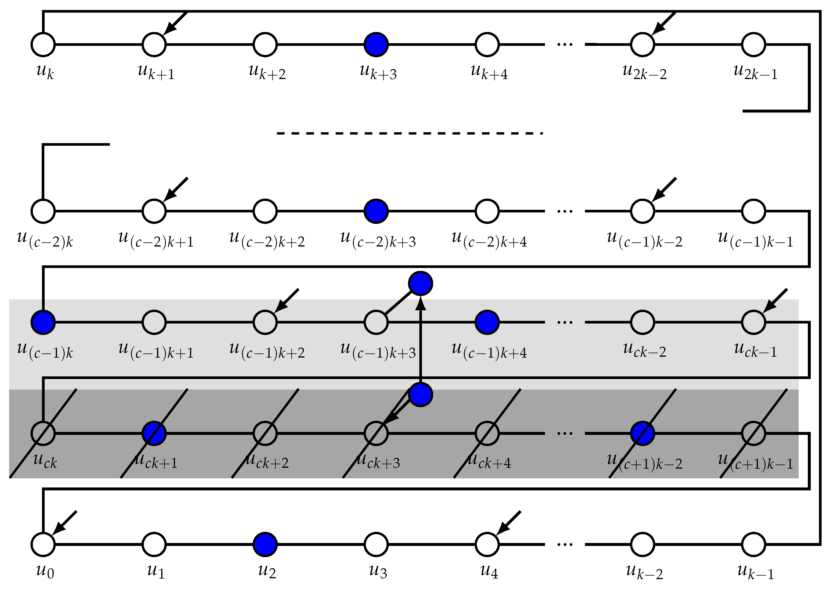
According to Proposition 3, we know that $P(ck,k)$ can be obtained from $P\left(\right(c+1)k,k)$ by Construction 1.

Proposition 7.

If $k\equiv 1mod2$, and $c\equiv 3mod4$, then ${\gamma }_{dR}\left(P(ck,k)\right)<\frac{3}{2}(c+\frac{1}{2})k$.

Proof. 

Let $c=4h-1$ and let f be the double Roman dominating function of $P\left(\right(c+1)k,k)=P(4hk,k)$ as defined above. Recall Construction 1 and note that ${\displaystyle V\left(P((c+1)k,k)\right)={\cup }_{i=0}^c(V_i\cup U_i)}$ and ${\displaystyle V\left(P(ck,k)\right)={\cup }_{i=0}^{c-1}(V_i\cup U_i)}$.

First assume, that $k\equiv 3mod4$. Define $\tilde{f}$ on $V\left(P\right(ck,k\left)\right)$ as follows.

• $\tilde{f}\left(x\right)=f\left(x\right)$ for $x\in V\left(P(ck,k)\right)\backslash (V_{c-1}\cup U_{c-1})$.
• For $x\in V_{c-1}\cup U_{c-1}$, observe that $x=u_{(c-1)k+i}$ or $x=v_{(c-1)k+i}$ for some $i=0,1,...,k-1$, and define

  $$\begin{array}{ccc}\hfill \tilde{f}\left(v_{(c-1)k+i}\right)& =& f\left(v_{(c-1)k+i}\right)+f\left(v_{ck+i}\right)\mathrm{and}\hfill \\ \hfill \tilde{f}\left(u_{(c-1)k+i}\right)& =& f\left(u_{(c-1)k+i}\right).\hfill \end{array}$$

It is straightforward to observe that, by definition, $\tilde{f}$ dominates all vertices on the inner cycle. On the outer cycle, the only interesting part are vertices $\{u_{ck-3},u_{ck-2},$$u_{ck-1},u_0,u_1,u_2\}$. By the basic assignment (see Equation (7)), we know that $\tilde{f}\left(u_2\right)=f\left(u_2\right)=3$, and $\tilde{f}\left(u_{ck-3}\right)=f\left(u_{ck-3}\right)=3$. Furthermore, $u_{ck-1}$ and $u_0$ are dominated by $\tilde{f}$, because $\tilde{f}\left(v_{ck-1}\right)=3$ and $\tilde{f}\left(v_0\right)=3$. See Figure 4 below. We conclude that $\tilde{f}$ is a double Roman dominating function of $P(ck,k)$.

Now recall that, by Proposition 6, if $k\equiv 3mod4$ then $w\left(f\left(U_c\right)\right)=3(\ell +1)>\frac{3}{4}k,$ and $w\left(f\left(V_c\right)\right)=3\ell <\frac{3}{4}k.$ It follows that $w\left(\tilde{f}\right)<\frac{3}{2}(c+\frac{1}{2})k$, as needed.

The case $k\equiv 1mod4$ can be treated similarly. Instead of D, $D^s$ is used (with $s=1$). We omit the details. □

5.3. Case $c\equiv$ 2 mod 4

According to Proposition 3, we know that $P(ck,k)$ is obtained from $P\left(\right(c+2)k,k)$ by Construction 1.

Proposition 8.

If $k\equiv 1mod2$, and $c\equiv 2mod4$, then ${\gamma }_{dR}\left(P(ck,k)\right)<\frac{3}{2}(c+\frac{2}{3})k$.

Proof. 

Let $c=4h-2$ and let f be the double Roman dominating function of $\left(P\right((c+2)k,k\left)\right)$ as defined above.

Define $\tilde{f}$ on $V\left(P\right(ck,k\left)\right)$ as follows. (Recall that Construction 1 was applied twice.)

• $\tilde{f}\left(x\right)=f\left(x\right)$ for $x\in {\cup }_{i=0}^{c-1}{U}_i$
• $\tilde{f}\left(x\right)=f\left(x\right)$ for $x\in {\cup }_{i=1}^{c-2}{V}_i$
• For $x\in V_0$, let $x=v_i$, $i=0,1,\dots ,k-1$ and set $\tilde{f}\left(v_i\right)=f\left(v_i\right)+\frac{2}{3}f\left(v_{(c+1)k+i}\right)$
• For $x\in V_{c-1}$, let $x=v_{(c-1)k+i}$, $i=0,1,\dots ,k-1$ and set $\tilde{f}\left(v_{(c-1)k+i}\right)=f\left(v_{(c-1)k+i}\right)+\frac{2}{3}f\left(v_{ck+i}\right)$

Observe that, by construction, $\tilde{f}$ is a double Roman dominating function of $P(ck,k)$.

To compute the weight of $\tilde{f}$, recall that by Proposition 6

$$w\left(f\left(U_{c-1}\right)\right)+w\left(f\left(U_c\right)\right)>w\left(f\left(V_{c-1}\right)\right)+w\left(f\left(V_c\right)\right)$$

and hence

$$w\left(f\left(V_{c-1}\right)\right)+w\left(f\left(V_c\right)\right)<\frac{1}{2}3k<w\left(f\left(U_{c-1}\right)\right)+w\left(f\left(U_c\right)\right);$$

thus, the total additional weight assigned is $\frac{2}{3}\left(\frac{1}{2}3k\right)=k$, because the weights transferred were multiplied by $\frac{2}{3}$. It follows that $w\left(\tilde{f}\right)<\frac{3}{2}(c+\frac{2}{3})k$, as claimed (see Figure 5). □

5.4. Case $c\equiv$ 1 mod 4

According to Proposition 3, we know that $P(ck,k)$ can be obtained from $P\left(\right(c+3)k,k)$ by Construction 1, applied three times.

Proposition 9.

If $k\equiv 1mod2$, and $c\equiv 1mod4$, then ${\gamma }_{dR}\left(P(ck,k)\right)<\frac{3}{2}(c+\frac{1}{2})k$.

Proof. 

Let $c=4h-3$ and f be the double Roman dominating function of $\left(P\right((c+3)k,k\left)\right)$ as defined above.

Recall Construction 1 and assume $k\equiv 3mod4$. Define $\tilde{f}$ on $V\left(P\right(ck,k\left)\right)$ as follows.

• $\tilde{f}\left(x\right)=f\left(x\right)$ for $x\in V\left(P(ck,k)\right)\backslash (V_{c-1}\cup U_{c-1})$
• For $x\in V_{c-1}\cup U_{c-1}$, observe that $x=u_{(c-1)k+i}$ or $x=v_{(c-1)k+i}$ for some $i=0,1,...,k-1$, and define

  $$\begin{array}{ccc}\hfill \tilde{f}\left(v_{(c-1)k+i}\right)& =& f\left(v_{(c-1)k+i}\right)+f\left(v_{(c+2)k+i}\right)\mathrm{and}\hfill \\ \hfill \tilde{f}\left(u_{(c-1)k+i}\right)& =& f\left(u_{(c-1)k+i}\right).\hfill \end{array}$$

Observe that, by construction, $\tilde{f}$ is a double Roman dominating function of $P\left(\right(c-3)k,k)$ and $w\left(\tilde{f}\right)<\frac{3}{2}(c+\frac{1}{2})k$, as needed (see Figure 6). We omit the details.

The case $k\equiv 1mod4$ is analogous. We skip the details. This completes the proof. □

6. Even k

For even k, we start with DRD functions for $P\left(c\right(k+1),k+1)$ constructed in the previous considerations (Propositions 5–9). The upper bounds for ${\gamma }_{dR}\left(P(ck,k)\right)$ for k even will be established by using the next observation.

Proposition 10.

Assume f is a DRDF for $P\left(c\right(k+1),k+1)$. Then there is a DRDF $\tilde{f}$ for $P(ck,k)$ of weight $w\left(\tilde{f}\right)\le (k+\frac{1}{2})\frac{1}{k+1}w\left(f\right)$.

Proof. 

Let f be a DRDF for $P\left(c\right(k+1),k+1)$. Recall Construction 2. By Proposition 4, if we choose any $K\in \{0,1,\dots ,k\}$, delete the inner cycle $In{n}_K=\left\{v_{jk+K}\right|j=0,1,2,\dots ,c\}$, $K\in \{0,1,\dots ,k\}$, and the corresponding K-th “column” of vertices $Ou{t}_K=\left\{u_{jk+K}\right|j=0,1,2,\dots ,c\}$, we obtain a graph that is isomorphic to $P(ck,k)$.

Define a DRDF $\tilde{f}$ on $P(ck,k)$, using the original labeling of $P\left(c\right(k+1),k+1)$, as follows.

• $\tilde{f}\left(x\right)=f\left(x\right)$ for $x\in P(c(k+1),k+1)\backslash (Ou{t}_{K-1}\cup In{n}_{K-1}\cup Ou{t}_K\cup In{n}_K)$.
• For $x\in Ou{t}_{K-1}$ we know that $x=u_{jk+K-1}$ for some j and define $\tilde{f}\left(x\right)=f\left(u_{jk+K-1}\right)+f\left(u_{jk+K}\right)$.
• For $x\in In{n}_{K-1}$ we know that $x=v_{jk+K-1}$ for some j and define $\tilde{f}\left(x\right)=f\left(v_{jk+K-1}\right)$.

Recall that the basic double Roman dominating partition for $P(ck,k)$ with $c=4h$ and k odd was higly symmetrical, in the sense that $w\left(In{n}_i\right)=w\left(Ou{t}_i\right)=\frac{3}{4}c$. Furthermore, in the proofs of Propositions 7–9, DRDF’s were constructed such that the property $w\left(In{n}_i\right)\ge w\left(Ou{t}_i\right)$ was preserved. Therefore, we can choose K such that the weight of the inner cycle is not under average, i.e., $w\left(f\left(In{n}_K\right)\right)\ge \frac{1}{2(k+1)}w\left(f\right)$.

We conclude that, by construction, $\tilde{f}$ is a double Roman dominating function of $P(ck,k)$, and

$$w\left(\tilde{f}\right)\le w\left(f\right)-\frac{1}{2(k+1)}w\left(f\right)=(k+\frac{1}{2})\frac{1}{k+1}w\left(f\right),$$

as needed. □

The Proposition just proved directly implies the next statement.

Proposition 11.

${\gamma }_{dR}\left(P(ck,k)\right)\le (k+\frac{1}{2})\frac{1}{k+1}{\gamma }_{dR}\left(P(c(k+1),k+1)\right)$,

We are now ready to prove the upper bounds in case k is even.

Proposition 12.

Let $k\equiv 0mod2$, then

1.

If $c\equiv 0mod4$, then ${\gamma }_{dR}\left(P(ck,k)\right)\le \frac{3}{2}c(k+\frac{1}{2})$.

2.

If $c\equiv 1mod4$, then ${\gamma }_{dR}\left(P(ck,k)\right)\le \frac{3}{2}(c+\frac{1}{2})(k+\frac{1}{2})$.

3.

If $c\equiv 2mod4$, then ${\gamma }_{dR}\left(P(ck,k)\right)\le \frac{3}{2}(c+\frac{2}{3})(k+\frac{1}{2})$.

4.

If $c\equiv 3mod4$, then ${\gamma }_{dR}\left(P(ck,k)\right)\le \frac{3}{2}(c+\frac{1}{2})(k+\frac{1}{2})$.

Proof. 

By Proposition 5 we have ${\gamma }_{dR}\left(P(c(k+1),k+1)\right)=\frac{3}{2}c(k+1)$ for $c\equiv 0mod2$ and $k+1\ge 1$ odd. From the proof of Proposition 5, we have explicit definition of a ${\gamma }_{dR}$-function f, with the property that $w\left(f\left(U_i\right)\right)=w\left(f\left(V_i\right)\right)=3\frac{k+1}{4}$ for all i. By Proposition 10, there is a DRD function $\tilde{f}$ $w\left(\tilde{f}\right)\le (k+\frac{1}{2})\frac{1}{k+1}w\left(f\right)$. Hence ${\gamma }_{dR}\left(P(ck,k)\right)\le \frac{3}{2}c(k+\frac{1}{2})$.

The other three cases follow from Propositions 7–9 by analogous reasoning. □

7. Conclusions and Future Work

Based on the previously known constructions of DRDF’s for $P(4k,k)$, the upper bounds for double Roman domination numbers of $P(ck,k)$ were derived, using the notion of graph covers and some new constructions of DRDF’s.

It may be of interest to compare the upper bounds of Theorem 1 with the bounds given by Gao et al. [12] (see Table 2). Let us take $n=ck$ and compare the following cases based on formula by Gao et al. below.

1.

Case $k\equiv 1mod2,n\equiv 0mod4$. Both formulas give exact value.

2.

Case $k\equiv 1mod4,n\not\equiv 0mod4$. Theorem 1 gives either $\frac{3k}{2}(c+\frac{1}{2})$ or $\frac{3k}{2}(c+\frac{2}{3})$ depending on c. As

$$\frac{3k}{2}(c+\frac{1}{2})<\frac{3k}{2}(c+\frac{2}{3})=\frac{3ck}{2}+k<\frac{3ck}{2}+\frac{5k+5}{4},$$

we conclude that Theorem 1 improves the upper bound of [12] in these cases.

3.

Case $k\equiv 3mod4,n\not\equiv 0mod4$. Reasoning along the same lines as in the previous case shows that Theorem 1 also improves the upper bound of [12] in these cases.

4.

Case $k\equiv 0mod4,n\equiv 0mod(3k+1)$. As we assume $n=ck$, it follows that we must have $n\equiv 0mod4$ and c must be odd. Theorem 1 thus assures the upper bound ${\gamma }_{dR}\left(P(ck,k)\right)<\frac{3}{2}(c+\frac{1}{2})(k+\frac{1}{2})=\frac{3}{2}ck+\frac{3}{4}c+\frac{3}{4}k+\frac{3}{8}$. Because $\frac{3ck}{2}\frac{(3k+2)}{(3k+1)}=\frac{3ck}{2}(1+\frac{1}{3k+1})=\frac{3ck}{2}+\frac{c}{2}\frac{3k}{(3k+1)}<\frac{3ck}{2}+\frac{c}{2},$ we conclude that in this case the upper bound in Theorem 1 does not improve the general bound of [12].

5.

Case $k\equiv 0mod4,n\not\equiv 0mod(3k+1).$ Now we cannot extract any condition on c so we compare $\lceil \frac{3ck}{2}\frac{(3k+2)}{(3k+1)}\rceil +\frac{5k+4}{4}$ with the upper bound $\frac{3}{2}(c+\frac{2}{3})(k+\frac{1}{2})=\frac{3}{2}ck+\frac{3}{4}c+k+\frac{1}{2}$ and conclude that for large enough k, the upper bound of Theorem 1 is better, whereas for the large c, the bound of [12] is not improved.

6.

Case $k\equiv 2mod4,n\equiv 0mod(3k-1)$. Compare $\frac{3ck}{2}\frac{\left(3k\right)}{(3k-1)}=\frac{3}{2}ck+\frac{3k}{(3k-1)}\frac{c}{2}$ with $\frac{3}{2}c(k+\frac{1}{2})=\frac{3}{2}ck+\frac{3}{4}c$ to conclude that in this case, the bound of Theorem 1 does not improve the general bound.

7.

Case $k\equiv 2mod4,n\not\equiv 0mod(3k-1)$. In this case, comparing $\lceil \frac{3n}{2}\frac{\left(3k\right)}{(3k-1)}\rceil +\frac{5k+6}{4}=\lceil \frac{3}{2}ck+\frac{3k}{(3k-1)}\frac{c}{2}\rceil +\frac{5k+6}{4}$ and $\frac{3}{2}(c+\frac{2}{3})(k+\frac{1}{2})=\frac{3}{2}ck+\frac{3}{4}c+k+\frac{1}{2}$ leads to the conclusion that Theorem 1 improves the general bounds for large enough k, and that for large c, the bound of [12] is not improved.

We can thus conclude that Theorem 1 in several cases improves the previously known general upper bound. The new bounds hold for all c and k, and are asymptoticaly the best possible, as the following corollary formally states.

Corollary 1.

For the double Roman domination number of generalized Petersen graphs $P(ck,k)$ of large graphs the following holds.

(1)

${\displaystyle \frac{3}{4}c\le \underset{k\to \infty }{lim}\frac{{\gamma }_{dR}\left(P(ck,k)\right)}{2k}\le \frac{3}{4}(c+\epsilon )}$, where $\epsilon =0,\frac{1}{2},\frac{2}{3},\frac{1}{2}$ when $c\equiv 0,1,2,3mod4$.

(2)

${\displaystyle \frac{3}{4}k\le \underset{c\to \infty }{lim}\frac{{\gamma }_{dR}\left(P(ck,k)\right)}{2c}\le \frac{3}{4}(k+\epsilon )}$, where $\epsilon =kmod2$.

(3)

${\displaystyle \underset{c\to \infty ,k\to \infty }{lim}\frac{{\gamma }_{dR}\left(P(ck,k)\right)}{2ck}=\frac{3}{4}}$.

The proof of Corollary 1 follows from Theorem 1.