Generalized Type-2 Fuzzy Parameter Adaptation in the Marine Predator Algorithm for Fuzzy Controller Parameterization in Mobile Robots

Abstract

This article is oriented to the application of generalized type-2 fuzzy systems in the dynamic adjustment of the parameters of a recent metaheuristic based on nature that follows the rules of the best feeding strategies of predators and prey in ecosystems. This metaheuristic is called fuzzy marine predator algorithm (FMPA) and is presented as an improved variant of the original marine predator algorithm (MPA). The FMPA balances the degree of exploration and exploitation through its iterations according to the advancement of the predator. In the state of the art, it has been shown that type-2 fuzzy increases metaheuristic performance when adapting parameters, although there is also an increase in the execution time. The FMPA with generalized type-2 and interval type-2 parameter adaptations was applied to a group of benchmark functions introduced in the competition on evolutionary computation (CEC2017); the results show that generalized FMPA provides better solutions. A second case for FMPA is also presented, which is the optimal fuzzy control design, in the search for the optimal membership function parameters. A symmetrical distribution of these functions is assumed for reducing complexity in the search process for optimal parameters. Simulations were carried out considering different degrees of noise when analyzing the performance when simulating each of the used fuzzy methods.

1. Introduction

In this article, a particular metaheuristic is considered: the marine predator algorithm (MPA), which can be considered a robust metaheuristic that has many advantages, for example, simple procedures, few design variables, flexibility, high level of convergence, almost global solution, and gradient-free attributes [1]. In addition, the MPA has been applied in diverse areas and has shown effective results, in which it has already been compared in previous studies in different problems, such as the prediction of COVID-19, and in control. Some of the studies that have considered this algorithm are the following: the first discussed a new integration between a neuro-fuzzy model and the marine predator optimization algorithm, with a search for optimal system parameters to increase biomethane gas production [2]. A hybrid computational intelligence approach for structural damage detection using the marine predator algorithm and feedforward neural networks is described in [3]. The following study implemented an MPA-based design for large-scale photovoltaic (PV) systems to achieve maximum power under partial shading conditions in [4]. The marine predator algorithm is proposed for solving transcendental nonlinear equations in a selective harmonic elimination technique using a multilevel inverter (MLI) [5]. In the search for the optimal values of the commutation angles with MPA, it is applied to control a three-phase motor of 11 levels using a cascade H-bridge (CHB) topology in the control of the fundamental component and cancel the low-order harmonics to all modulation index values from 0 to 1 [5]. The marine predator algorithm is used to optimize the gains as well as the input scaling factors and membership functions of a proposed fuzzy PID controller in [6]. A novel technique for multilevel thresholding of digital image segmentation by combining fuzzy entropy type-II (FE-TII) with a metaheuristic marine predator algorithm is proposed in [7]. A new short-term COVID-19 forecast model is proposed using an improved version of the adaptive neuro-fuzzy inference system (ANFIS); then an improved MPA, called chaotic MPA (CMPA), is applied to improve the ANFIS and avoid its deficiencies [8]. More recently, a hybrid COVID-19 detection model based on an improved marine predator algorithm (IMPA) and a ranking-based diversity reduction strategy is proposed for X-ray image segmentation with the aim of rapidly extracting from chest X-ray images the similar small regions that may contain the identifying features of COVID-19 [9].

Some researchers have proposed implementing the fuzzy logic controller (FLC) in parallel with conventional controllers to improve overall system performance [10,11,12,13]. A trend that has occurred in recent years is that fuzzy controllers are optimized using metaheuristic approaches and, in this way, optimally achieve a parameter setting and therefore reduce the proposed objective function since the best is not usually achieved [14,15]. Although these techniques can be very competitive, they do not necessarily obtain better times and computational costs with their application [16]. The fuzzy controller input variables are determined by combinations of membership functions known as fuzzy sets, and their parameter values can be metaheuristically tuned to produce the desired performance required by the system [17]. The area of fuzzy logic continues to advance, since recently an investigation was presented in which dynamic fractional order models are obtained from an extension to general type-2 fuzzy systems, which are called interval type-3 fuzzy logic systems (IT3FLS) [18].

In previous control investigations, different variants of algorithms have been presented to adapt the parameter values of the membership functions of the fuzzy controller, such as the hybrid harmony search and differential evolution algorithm for the optimal design of fuzzy controllers [19,20], and the optimization of type-2 and type-1 fuzzy controllers utilizing the shark smell optimization algorithm is described in [17]. In addition, to control an inverted pendulum system in [21], the optimal parameter estimation of a controller for an autonomous mobile robot for adjusting a fuzzy controller using the firefly algorithm is described in [22], and an optimization of interval type-2 fuzzy controllers with parameter adaptation utilizing fuzzy systems (of the interval type-2 and type-1 form) for the optimization of the fuzzy controller of an autonomous mobile robot is presented in [23]. In addition, fuzzy parameter adaptation of the grey wolf algorithm is offered in [24]. A variant of differential evolution applying shaded and general type-2 systems for adjustment of the main parameter of an evolutionary technique is presented in [25], a comparison applying the multiverse optimizer and also varying the parameter values of the principal points in each membership function, its comparison with other algorithms in the optimization of fuzzy controllers, and benchmark problems in [26], An improved hybrid IT2FLC design was proposed for the design of a fuzzy controller based on a variant of the shark smell and salp swarm algorithms with parameter adaptation for the benchmark problem of a DC motor. Additionally, test runs on CEC2017 benchmark functions are presented in [27].

Research has been developed that suggests the use of generalized type-2 fuzzy systems (GT2FLSs) in the control area or in other more complex endeavors. In addition, very few related works have been developed that apply optimization techniques to formulate an optimal GT2FLS. In addition, the concepts of GT2FLS and the representation of planes (α cuts) as a mechanism to increase their ability to find solutions to problems of different complexity have been recently applied [28,29,30,31,32,33]. It has been established in previous research how much type-2 fuzzy systems help when utilized, as they increase the performance of metaheuristics by dynamically adapting the parameters through their executions [34]. However, there is a limitation when using fuzzy logic in the variation of parameters that we get longer execution times for metaheuristics.

Therefore, the application of the FMPA metaheuristic in solving complex problems has been established with the guidance of previously referenced works as the main motivation of this research, since in the state of the art, there are few works that deal with metaheuristics inspired by nature and using parameter adjustment based on a GT2FLC. Appealing to the robustness, as a property of the GT2FLS, we use it as a tool to find the best values of the P, FADs, and CF parameters of the MPA algorithm.

The greatest contribution of this research, analyzing the divergence from previous works in the literature, was to develop a comparative analysis by taking the different types of FLSs, in the optimal tuning of the main parameters of the marine predator algorithm, for the functionality of fuzzy controllers and, finally, for the improvement of results for CEC2017 benchmark functions. Furthermore, the results obtained from the executions with the marine predator algorithm based on the adaptation of generalized type-2 FLC parameters show a great improvement. The generalized type-2 FLS (FMPAGT2) is by far more efficient than the original MPA algorithm and its fuzzy counterparts, the interval type-2 and type-1 FLS (FMPAIT2 and FMPAT1), in finding better parameter values.

Therefore, hybridization is an important contribution of this work, as GT2FLSs are combined with marine predator algorithm to propose a novel variant of MPA to help in the exploration of optimal fuzzy controllers and the optimal search for results in the CEC2017 benchmark functions. It was assumed that a goal was a better treatment and handling of uncertainty in optimization problems, in addition to presenting a comparison between T1FLC, IT2FLC, and GT2FLC for the development of optimal fuzzy controllers and the application of fuzzy systems in the search for the key parameter values in the marine predator algorithm implemented for the optimization of benchmark functions.

The composition of the document is as follows: Section 2 outlines a background of the types of fuzzy systems used in this work. Section 3 puts forward the proposal for the improvement on the optimization of fuzzy systems. Section 4 presents the case studies: CEC2017 benchmark functions and fuzzy controller design, in addition to the formulation of the objective function. Section 5 describes a compilation of results of experimentation with both case studies: CEC2017 benchmark functions and mobile robot fuzzy controller optimization. Section 6 offers conclusions and possible future works.

2. Fuzzy Systems

Fuzzy logic systems (FLSs) have advanced through the years since their inception in 1965 with a type-1 fuzzy logic system (T1FLS) to represent the vagueness in the real world, as a methodology for control, as well as the application of mathematical models to emulate human understanding, industrial developments, electronic applications, medical opinion systems, and robotics, to name a few. Later, due to the interest in managing uncertainties, what we now know as type-2 fuzzy logic did emerge, which has steadily evolved to the present day.

Although the area of fuzzy logic continues to advance, recently, an investigation was presented in which dynamic fractional-order models were obtained from an extension of general type-2 fuzzy systems, which are called interval type-3 fuzzy logic systems (IT3FLS), where the secondary membership function (SMF) is an interval type-2 fuzzy set (FS). Values of a tertiary membership are unity over the footprint of uncertainty (FOU) of secondary membership [35]. A proposed novel method based on interval type-3 fuzzy logic systems (IT3-FLSs), an online learning approach for solar energy management systems, is described in [18]. Finally, the design of an interval type-3 (IT3) Takagi–Sugeno (T-S) fuzzy logic system (FLS) using the alpha plane representation is presented in [34].

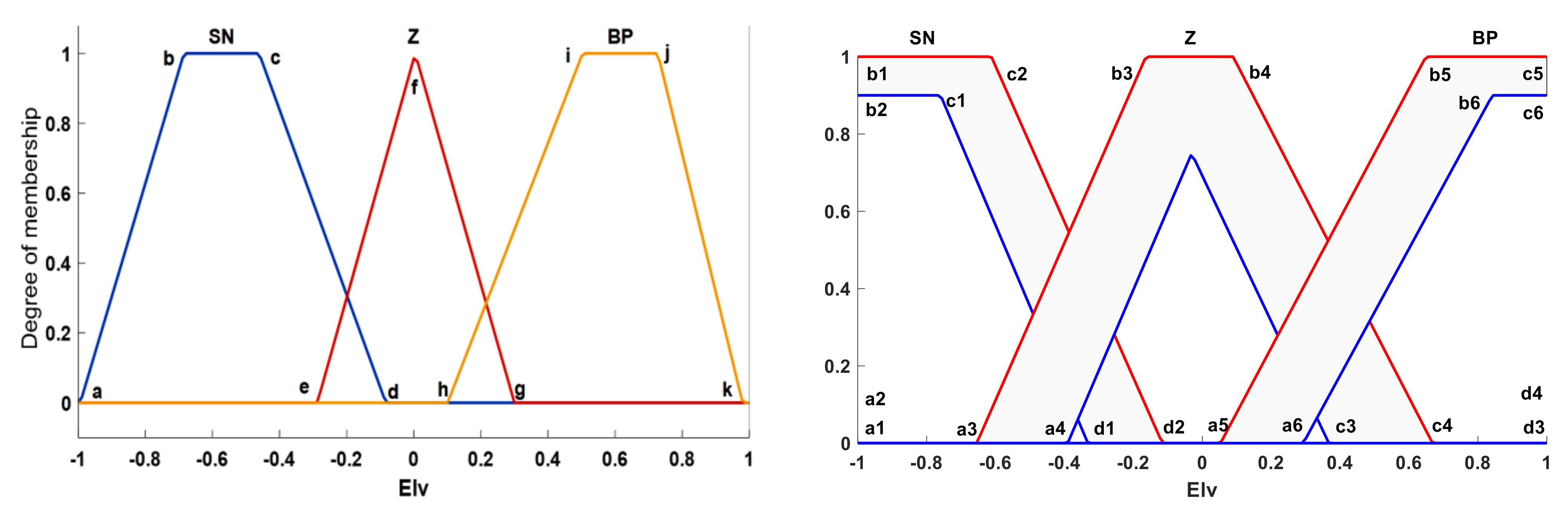
2.1. Type-1 Fuzzy Systems

Based on the foundations of fuzzy logic [36], we can define a fuzzy set (FS) characterized by the membership function (MF). This initial definition of a type-1 fuzzy set is expressed as: a fuzzy set is characterized by an MF ${\mu }_A\left(x\right)$ that has values on [0, 1] and can be interpreted as a set of pairs defined by Equation (1):

$$A=\left\{\left(x, {\mu }_A\left(x\right)\right)\right| x \in X\}$$

(1)

where ${\mu }_A$: X→ [0, 1]. Here, ${\mu }_A\left(x\right)$ represents the membership degree of the element x ∈X to the set A. Figure 1 depicts a type-1 fuzzy system, which is structured by the fuzzifier, the rules, the inference, and finally, the defuzzifier [37].

The fuzzifier performs the process of converting precise numbers to fuzzy sets, the inference process computes fuzzy rules based on the activation of the inputs, and finally, the defuzzifier performs the reverse process, converting the resulting fuzzy sets to precise numbers. Figure 2 illustrates the inference process of a Mamdani-type T1FIS. In the control area, the fuzzy systems have had a great boom due to their great ability to control nonlinear systems. Some examples of recent applications can be found in [14,36,37], having each day more applications in different areas, like to Robot control [38,39].

Given the inputs (numerical values), different membership values are obtained for each of the values. This represents an “input fuzzification”. If the premise of the rule contains more than one expression, we will apply an operator (t-norm or t-conorm) to obtain the activation of the rule. This is shown in the example in Figure 2.

Starting from the consequent of each rule in addition to the value of the obtained antecedent, we use a fuzzy implication operator, resulting in a new FS. One of the most used implication operators is the minimum, which cuts the MF of the consequent, and the product, which scales it.

The outputs resulting from each rule in step 2 are combined into a single fuzzy set using an aggregation operator. The most popular aggregation operators are the maximum, the sum, or the probabilistic or. In Figure 2, the maximum is utilized.

In the case of finding a solution to a decision problem, what we need as output is a number. Therefore, we have to transform the fuzzy set calculated in step 3 into a number. One of the most used methods is the centroid method that calculates the center of the area defined by the FS calculated in step 3. The calculation is shown in Figure 2.

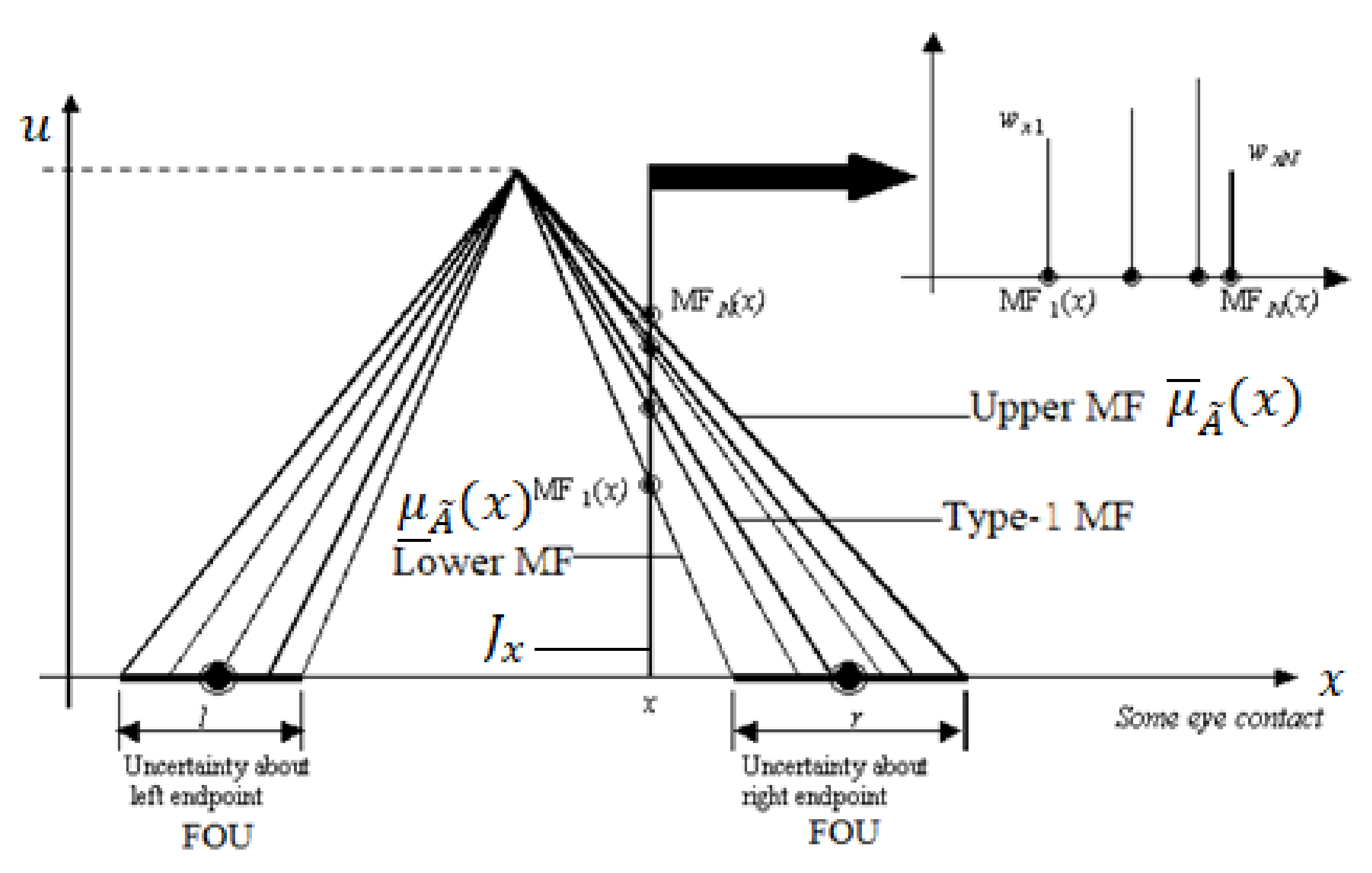
2.2. Interval Type-2 Fuzzy Systems

Based on Zadeh’s ideas, Mendel et al. introduced the definition of a type-2 fuzzy set [40,41]. Based on the initial concepts of FS [42,43], interval type-2 fuzzy sets (IT2FS) represent an uncertainty model [44] (see

Table 1. Formula for the upper and lower MFs.

FOU	${\mathit{\mu }}_{\overline{\mathit{A}}}^{ }\left(\mathit{x}\right)$	${\mathit{\mu }}_{\underset{\_}{\mathit{A}}}\left(\mathit{x}\right)$
	$F_{\overline{A}}^{ }\left(x\right)=\left\{ \begin{array}{c}0, x\le a\\ \frac{x-a}{b-a}, a<x\le b\\ 1, b<x\le c\\ \frac{d-x}{d-c}, c<x\le d\\ 0, x\ge d\end{array}\right.$	$F_{\underset{¯}{A}}\left(x\right)=\left\{ \begin{array}{c}0, x\le e\\ \frac{x-e}{f-e}, e<x\le f\\ \\ \frac{\mathrm{g}-x}{\mathrm{g}-f}, f<x\le g\\ 0, x>g\end{array}\right.$

). An IT2FS $\tilde{A}$ is represented by ${\underset{\_}{\mu }}_{\tilde{A}}\left(x\right)$ and ${\overline{\mu }}_{\tilde{A}}\left(x\right)$, the lower and upper MFs of ${\mu }_{\tilde{A}}\left(x,u\right)$, where $x\in X$, and $u\in J_x \subseteq \left[0, 1\right]$. Equation (2) describes the concept of an IT2FS [45]:

$$\tilde{A}=\left\{\left(\left(\mathrm{x}, \mathrm{u}\right), {\mu }_{\tilde{A}}\left(x,u\right)\right)\right| \forall x \in X, \forall u \in J_x \subseteq \left[0, 1\right]\}$$

(2)

where X is the primary domain, and $J_x$ is the the secondary domain of the primary memberships, which is the secondary domain. All secondary degrees ${\mu }_{\tilde{A}}\left(x,u\right)$ are equal to 1 representing the membership degree of each element. Figure 3 illustrates and represents an IT2FLS.

An MF of type IT2 can be represented as two T1 MFs, described as upper MF and lower MF, and the extension between them is recognized as the footprint of uncertainty (FOU) [46,47], and Figure 3 illustrates this representation.

What also characterizes an IT2FLS are the IF-THEN control rules; what differentiates it are its fuzzy sets that now have the form of a type-2 interval. A T2FS can be used when the events are too ambiguous to specify the relationship with exact degrees of membership, as in a fuzzy controller, where the membership functions take on many values, and we seek to determine the assignment of the best MF features that give optimal results and a stable controller [48] and function optimization [49].

The main difference in an IT2FS is that it includes a type-reducer module to summarize an IT2FS to a T1FS, and later is presented in the defuzzifier module, obtaining a crisp result [40]. The IT2FLS takes the uncertainty or ambiguity in the system, while the T1FLS just does not do it properly [41]. Although it is similar to a T1FLS, a block diagram presented in Figure 4 describes an IT2FLS.

In this work, we used the architecture of the fuzzy system, as described in Figure 4. For all inputs p and rule l, we are using MFs with an uncertain mean. The upper and lower MFs for the IT2FS are described in Table 1.

Taking into account that we formulate N rules on a rule base of T2FLC, these are with the form [41] of Equations (3) and (4):

$$R^l:If x_1 is {\tilde{F}}_{\mathrm{i}}^l and \dots , x_p is {\tilde{F}}_p^l then y is G_{ }^l,\hspace{1em}\hspace{1em}\hspace{1em}\hspace{1em} l=1,\dots ,N$$

(3)

where $x_i\left(i=1,..p\right)$ are inputs and ${\tilde{F}}_{\mathrm{i}}^l$ are antecedent sets, $G_{ }^l$ are consequent sets, $y$ is the output variables, and ‘~’ implies that the set is a type-2 fuzzy set.

The firing strength is the following set of type-2 intervals:

$$F^i\left(x\right)=[ {\underset{\_}{f}}^i{}_{ }^{ }\left(x\right),{\overline{f}}^i\left(x\right) \equiv \left[ {\underset{\_}{f}}^i,{\overline{f}}^i\right]]$$

(4)

There are different techniques for the implementation of an IT2FLS type reducer, where the center of gravity (cos) is one of the most used techniques, where $y_{COS}$ is an interval, described by the values $y_l^i,y_r^i$, which are computed with Equations (5) and (6). Karnik and Mendel [43] showed that the two endpoints $y_l$ and $y_r$ depend on a combination of ${\underset{\_}{f}}_i$ and ${\overline{f}}_i$ values.

$$\begin{array}{c} y_l=y_l\left({\overline{f}}^1,\dots ,{\overline{f}}^N,{\underset{\_}{f}}^{L+1},\dots ,{\underset{\_}{f}}^N,y_l^1,\dots ,y_l^N\right) \\ y_r=y_r\left({\underset{\_}{f}}^1,\dots ,{\underset{\_}{f}}^N,{\overline{f}}^{R+1},\dots ,{\overline{f}}^N,y_r^1,\dots ,y_r^N\right)\end{array}$$

(5)

Here, ${\overline{f}}_j$ and ${\underset{\_}{f}}_j$ are upper and lower values of F, and Karnik and Mendel developed an iterative process for computing the values of $y_l$ and $y_{r.}$

$${\mu }_{{\tilde{A}}_k^i}\left( x_k\right)=\left[{\underset{\_}{\mu }}_{{\tilde{A}}_k^i}\left( x_k\right), {\overline{\mu }}_{{\tilde{A}}_k^i}\left( x_k\right)\right]=\left[{\underset{\_}{\mu }}^i, {\overline{\mu }}^i\right]$$

(6)

They proposed an algorithm that finds the switch points L and R and calculates the end points $y_l$ and $y_r$ of a type-reduced set in the following way:

$$y_l=\frac{{{\displaystyle \sum }}_{i=1}^L\overline{f_i}{y}_i^l+{{\displaystyle \sum }}_{i=L+1}^N\underset{\_}{f_i}{y}_i^l}{{{\displaystyle \sum }}_{i=1}^L{\overline{f}}_i+{{\displaystyle \sum }}_{i=L+1}^N\underset{\_}{f_i}}$$

(7)

$$y_r=\frac{{{\displaystyle \sum }}_{i=1}^R\underset{\_}{f_i}{y}_i^r+{{\displaystyle \sum }}_{i=R+1}^N\overline{f_i}{y}_i^r}{{{\displaystyle \sum }}_{i=1}^R\underset{\_}{f_i}+{{\displaystyle \sum }}_{i=R+1}^N\overline{f_i}}$$

(8)

Here, with the Karnik–Mendel algorithm (

Table 2. Karnik–Mendel algorithm.

Step	Left Point	Right Point
1	Sort $x_i$ by increasing order	Sort $x_i$ by increasing order
2	Initialize $w_i$ as: $w_i=\frac{{\overline{w}}_i+{\underset{\_}{w}}_i}{2}$	Initialize $w_i$ as: $w_i=\frac{{\underset{\_}{w}}_i+{\overline{w}}_i}{2}$
3	Compute $y=\frac{{{\displaystyle \sum }}_{i=1}^N{x}_i{w}_i}{{{\displaystyle \sum }}_{i=1}^N{w}_i}$	Compute $y=\frac{{{\displaystyle \sum }}_{i=1}^N{x}_i{w}_i}{{{\displaystyle \sum }}_{i=1}^N{w}_i}$
4	Find $k$ where $x_k<y<x_{k+1}$	Find $k$ where $x_k<y<x_{k+1}$
5	Set $w_i=\left\{\begin{array}{c}{\overline{w}}_i, i\le k\\ {\underset{\_}{w}}_i, i>k\end{array}\right.$	Set $w_i=\left\{\begin{array}{c}{\underset{\_}{w}}_i, i\le k\\ {\overline{w}}_i, i>k\end{array}\right.$
6	Compute $y=\frac{{{\displaystyle \sum }}_{i=1}^N{x}_i{w}_i}{{{\displaystyle \sum }}_{i=1}^N{w}_i}$	Compute $y=\frac{{{\displaystyle \sum }}_{i=1}^N{x}_i{w}_i}{{{\displaystyle \sum }}_{i=1}^N{w}_i}$
7	If, then stop, set, and if not, go to step 8	If, then stop, set, and if not, go to step 8
8	Go to step 3	Go to step 3

), the change points can be calculated. Finally, the crisp outputs in the defuzzification process can be evaluated as:

$$y=\frac{y_l+y_r}{2}$$

(9)

Here, $y$ is a defuzzified output. The Karnik–Mendel algorithm is not too time-consuming, and it is efficient for the application of T2FLSs.

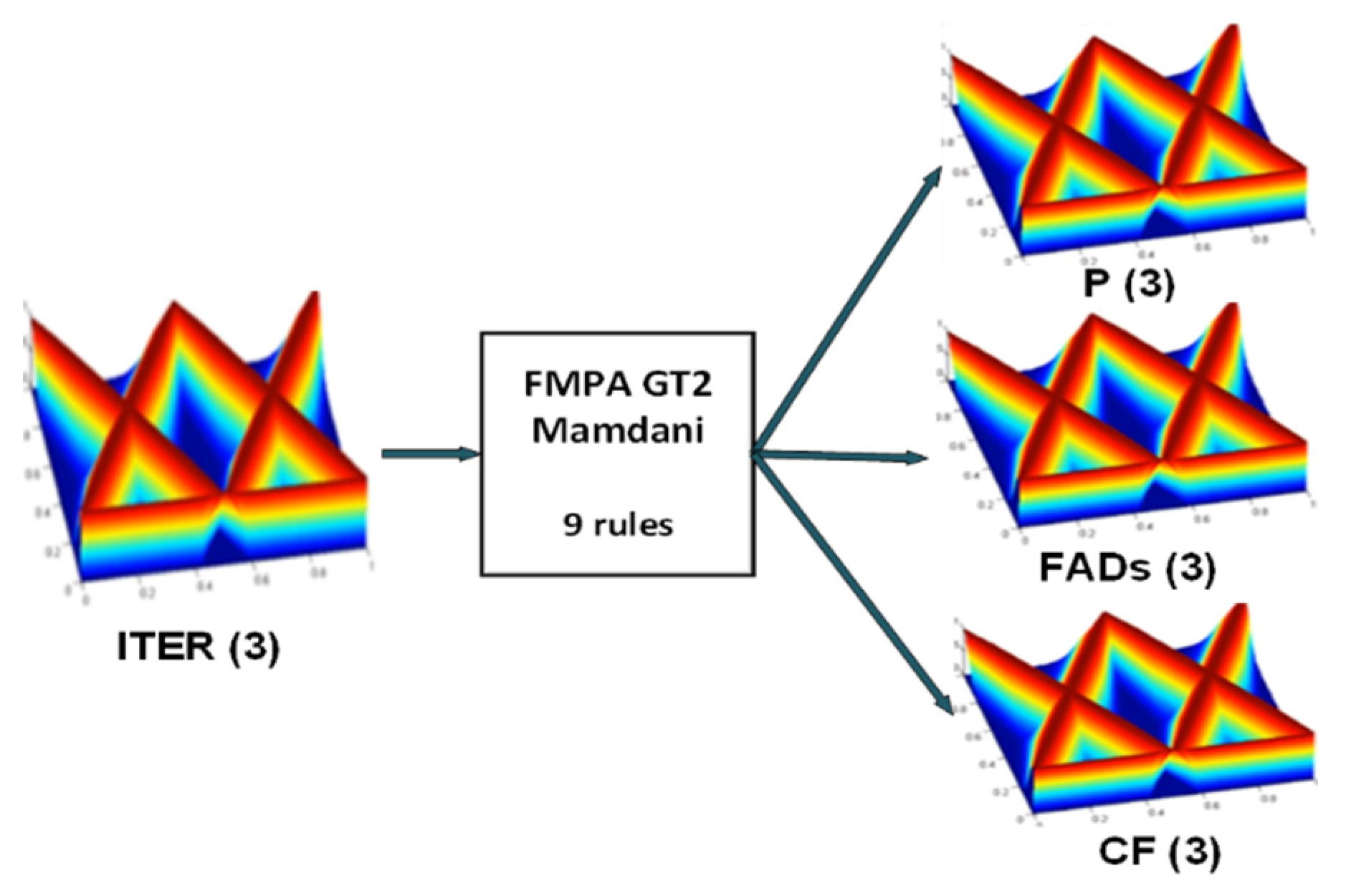
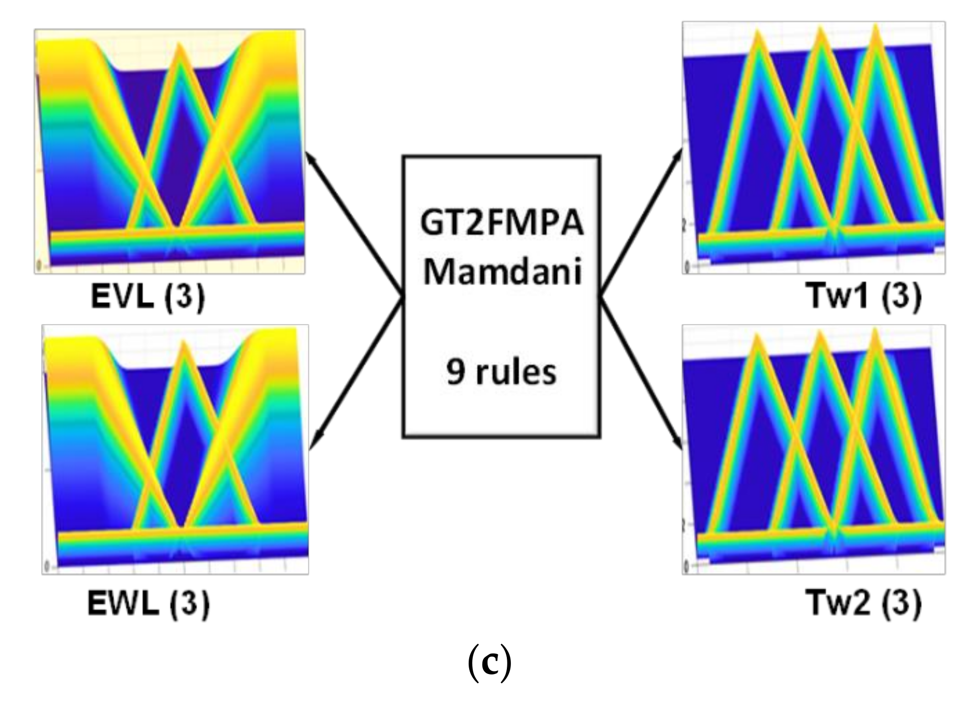
2.3. Generalized Type-2 System

The GT2FLS was determined approximately in 1999; however, its practical use has been impeded by its greater computational complexity, favoring the simplest version, the IT2FLS. The logic that is applied in IT2FLSs and T1FLSs is similar to that used in a GT2FLS, only that there is relatively more complexity in its procedure and operations [30]. Figure 5 describes a membership function using an example of a generalized type-2 Gaussian illustrated from various angles, which is showing the relationship with a third dimension and presents a better approximation to uncertainty.

The difference of a GT2FLS is due to the need to utilize the vertical axis, where the main reason lies in the complexity involved in the GT2FLS compared with the less complex fuzzy sets in T1FLSs and IT2FLSs [50,51].

Equation (10) describes the function of the generalized T2 fuzzy set:

$$\tilde{A}=\left\{\left( \right.\left(x,u\right), {\mu }_{\tilde{A}}\left(x, u\right)\left. \right)\left|{\forall }_x ϵ X,\right.\right.{\forall }_u \in J_{x }\subseteq \left[0, 1\right]\left. \right\}$$

(10)

where $J_{x }\subseteq \left[0, 1\right]$, x is in the domain of the primary MF, and $u$ is in the domain of the secondary MF.

Figure 6 describes the architecture of a GT2FLS in a more synthesized and stylized way.

2.3.1. The Fuzzification Stage

The generalized fuzzy set, in its fuzzification stage, has a single non-zero member-ship point. So the singleton fuzzy block interprets the crisp input $x_P$ into a Type-2 fuzzy singleton, whose MF is ${\mathsf{\mu }}_{{ \tilde{\mathrm{A}}}_{\mathrm{p}} }\left({\mathrm{x}}_{\mathrm{p}}\right)=\raisebox{1ex}{$1$}\!\left/ \!\raisebox{-1ex}{$1$}\right.{ \mathrm{for} \mathrm{x}}_{\mathrm{p}}={\mathrm{x}}_{\mathrm{p}}^{\prime }{ \mathrm{and} \mathsf{\mu }}_{{ \tilde{\mathrm{A}}}_{\mathrm{p}} }\left({\mathrm{x}}_{\mathrm{p}}\right)=0{ \mathrm{for} \mathrm{all} \mathrm{x}}_{\mathrm{p}}\ne {\mathrm{x}}_{\mathrm{p}}^{\prime } \mathrm{for} \mathrm{all} \mathrm{p}=1, 2, \dots ,\mathrm{P}, \mathrm{where} \mathrm{P} \mathrm{is} \mathrm{the} \mathrm{number} \mathrm{inputs}$ [52].

2.3.2. The Inference Stage

This stage introduces the interpretation of the rule base configuration; it is used in a GT2FLS using the definition of Mamdani-type rules, similar to those described for a T1FLS and IT2FLS. In this case, the antecedents and the consequent are characterized for a GT2FLS. Therefore, there are K rules defined, and the $k_{th}$ rule in the GT2FLS can be formulated by means of Equation (11) [20,32] and defines the relationship between the input and output fields.

$$R^{k}k: \mathit{IF} x_1 \mathit{is}{\tilde{F}}_1^k \mathit{and} \dots \mathit{and} x_p \mathit{is} {\tilde{F}}_p^k, \mathit{THEN} y \mathit{is} {\tilde{G}}^k$$

(11)

where $R^k$ is a specific rule, $x_p$ is the input $p$, ${\tilde{F}}_p^k$ is an MF on rule $y$ and the input $p$, and $y$ is the output on MF ${\tilde{G}}^k$. Both ${\tilde{F}}_1^k$ and ${\tilde{G}}^k$ are in the forms ${\mu }_F\left(x\right)$ and ${\mu }_G\left(y\right)$, respectively.

The inference of the rules is generated with Equations (12) and (13) by means of the t-norm connectors ($\tilde{\ast }$), where ${\mu }_{\tilde{B}}$ defines the membership function that arises in the consequents when inferring each rule, and w corresponds to the space of the consequents. The GT2FLS is used in the inference process, which involves two procedures identified as meet and join. These are formulated in Equations (12) and (13), respectively.

$${\mu }_{\tilde{A}}(x, u) ⨆ {\mu }_{\tilde{B}}(x, w)=\{\left(v, f_x\left(u\right) \tilde{\ast } f_x\left(w\right)\right) | v \in u \vee w, u\in J_x^u \subseteq [0, 1], w\in J_x^w \subseteq [0, 1]\}$$

(12)

$${\mu }_{\tilde{A}}\left(x, u\right) ⨅ {\mu }_{\tilde{B}}\left(x, w\right)=\{ \left(v, f_x\left(u\right) \tilde{\ast } f_x\left(w\right)\right) | v \in u \bigwedge w, u \in J_x^u \subseteq \left[0, 1\right], w \in J_x^w \subseteq \left[0, 1\right]\}$$

(13)

2.3.3. Interpretation of α-Planes

The interpretation of an α-plane for a GT2FLS ($\widetilde{A }$) takes the following form: it is denoted by ${\widetilde{A }}_{\propto }$, and it is postulated as the union of all primary MFs of $\widetilde{A }$, whose secondary memberships are higher than or equal to $\alpha \left(0 \le \alpha \le 1\right)$ [40,41]. The definition for the α-plane is described by Equation (14), and Figure 7 depicts a particular case of an α-plane [20,28].

$${\widetilde{A }}_{\mathsf{\alpha }}=\left\{\right(\mathrm{x}, u), {\mu }_{\tilde{A}}(x, u) \ge \mathsf{\alpha }|\forall x\in X, \forall u\in J_X \subseteq [ 0, 1\left]\right\}$$

(14)

2.3.4. Type Reduction

Regarding the type reducer that is applied to a GT2FLS, the most used technique is the centroid, described by Equation (15), taking it as the definition of the centroid $C_{\widetilde{A }}$ of a GT2FLS. ${\theta }_i$ represents the changes in relation to the secondary degree of the function $f_{x_1}\left({\theta }_1\right)\tilde{\ast }\dots \tilde{\ast }{f}_{x_N}\left({\theta }_N\right)$.

$$C_{\widetilde{A }}= \{(z, \mathsf{\mu }(z)) | z\in \frac{{{\displaystyle \sum }}_{i=1}^N{x}_i{\theta }_i}{{{\displaystyle \sum }}_{i=1}^N{\theta }_i}, \mathsf{\mu }\left(z\right) \in f_{x_1}({\theta }_1) \times ... \times f_{x_N}({\theta }_N), {\theta }_1 \in J_{x_1}\times ... \times J_{x_N}\}$$

(15)

One of the techniques for type reduction is the one developed by Karnik and Mendel [43], where ${ \overline{\mathsf{\Omega }}}_{\alpha }^k$ indicates the upper MFs’ alpha plane and ${ \underset{\_}{\mathsf{\Omega }}}_{\alpha }^k$ denotes the lowest alpha plane of the MF. Equations (16) and (17) condense this type reduction.

$$y_{\alpha }^l\left(x^{\prime }\right)=\frac{{{\displaystyle \sum }}_{k=1}^L{ \overline{\mathsf{\Omega }}}_{\alpha }^k\left(x^{\prime }\right)y_l^i+{{\displaystyle \sum }}_{j=L+1}^N{ \underset{\_}{\mathsf{\Omega }}}_{\alpha }^j\left(x^{\prime }\right){\overline{y}}_l^j}{{{\displaystyle \sum }}_{k=1}^L{ \overline{\mathsf{\Omega }}}_{\alpha }^k\left(x^{\prime }\right)+{{\displaystyle \sum }}_{j=L+1}^N{ \underset{\_}{\mathsf{\Omega }}}_{\alpha }^j\left(x^{\prime }\right)}$$

(16)

$$y_{\alpha }^r\left(x^{\prime }\right)=\frac{{{\displaystyle \sum }}_{k=1}^R{\mathsf{\Omega }}_{\alpha }^k\left(x^{\prime }\right)y_r^i+{{\displaystyle \sum }}_{k=R+1}^N{\mathsf{\Omega }}_{\alpha }^k\left(x^{\prime }\right){\overline{y}}_r^k}{{{\displaystyle \sum }}_{i=1}^R{ \underset{\_}{\mathsf{\Omega }}}_{\alpha }^i\left(x^{\prime }\right)+{{\displaystyle \sum }}_{i=R+1}^N{ \overline{\mathsf{\Omega }}}_{\alpha }^i\left(x^{\prime }\right)}$$

(17)

The process that continues is composed of the integration of the alpha planes, and Equations (18) and (19) describe the procedures necessary to achieve this [28,43].

$${\widehat{y}}_j^l\left(x^{\prime }\right)=\frac{{{\displaystyle \sum }}_{i=1}^N{\alpha }_i^{{\alpha }_i}{y}_j^l\left(x^{\prime }\right)}{{{\displaystyle \sum }}_{i=1}^N{\alpha }_i}$$

(18)

$${\widehat{y}}_j^r\left(x^{\prime }\right)=\frac{{{\displaystyle \sum }}_{i=1}^N{\alpha }_i^{{\alpha }_i}{y}_j^r\left(x^{\prime }\right)}{{{\displaystyle \sum }}_{i=1}^N{\alpha }_i}$$

(19)

2.3.5. The Defuzzification Stage

Once the type reduction operation has been carried out, the resulting values go to the defuzzification stage, which is obtained by the mean of $y_l$ and $y_r$. Equation (20) represents the defuzzified output of a nonsingleton GT2FLS [32,33].

$${\widehat{y}}_j\left(x^{\prime }\right)=\frac{{\widehat{y}}_j^l\left(x^{\prime }\right)+{\widehat{y}}_j^r\left(x^{\prime }\right)}{2}$$

(20)

3. Metaheuristic of Marine Predators

Now, in current research, it has become very common to apply metaheuristics when determining feasible solutions to problems in different areas, and they are used expecting to optimize the results of the problems. This research presents a recently created algorithm, its main qualities, and mathematical procedures for its implementation. The algorithm is the marine predator algorithm (MPA) with the implementation of GT2FLS for parameter adaptation. The combination between the GT2FLS and the marine predator algorithm is called FMPAGT2, which is a new variant proposed in this work (see Figure 8).

3.1. Marine Predator Algorithm

The marine predator’s algorithm (MPA) is a fairly recent proposed algorithm inspired by the actions of predator and prey in nature [1,2,3,4,5]. When presenting the proposed algorithm, it is very important to first know the mathematical model of the two main random movements on which this approach is based, the (i) Brownian movement and (ii) the Lévy movement.

3.1.1. Brownian Motion

The Brownian motion is the random motion observed in particles, where the trajectories developed by the Brownian particle are irregular (Equation (21)) and, of course, depend on the experimental observation times; that is, the sampling points on the path will not be the same as if the particle is observed in different time intervals.

It is a stochastic process in continuous time, where the extension of its step is extracted from a probability function determined by the normal distribution (Gaussian) with zero mean (μ = 0) and unit variance (${\sigma }^2$ = 1). The probability density function (PDF) that governs point $x$ for this movement is given by (Equation (21)):

$$f_B\left(x;\mu , \sigma \right)=\frac{1}{\sqrt{2\pi {\sigma }^2}}{e}^{\left(-\frac{{\left(x-\mu \right)}^2}{2{\sigma }^2}\right)}$$

(21)

Figure 9a shows how the Brownian motion covers more domain areas with more uniform and controlled steps, unlike the Lévy strategy.

3.1.2. Levy Movement

The probability density function of the Lévy distribution over the x$\ge \mu$ (Equation (22)) is defined as.

$$f_L\left(x; \mu , c \right)=\sqrt{\frac{c}{2\pi }} \frac{e^{-\frac{c}{2\left(x-\mu \right)}}}{{\left(x-\mu \right)}^{\frac{3}{2}}}$$

(22)

The side of this function exhibits heavy tail behavior that falls according to a power law (Equation (23)):

$$f_L\left(x; \mu , c \right)=\sqrt{\frac{c}{2\pi }} \frac{1}{x^{\frac{3}{2}}}, if x\to \infty$$

(23)

where $c$ is the scale parameter. This shows that Lévy not only has a tail, but also has a thick tail where $\mu =0$. Figure 9b shows that a Lévy flight is mainly related to small steps and occasional long jumps.

Therefore, predators take the Lévy strategy when there is a low conglomeration of prey and Brownian motions when there is prey abundance [2], where the velocity ratio v from the prey to the predators represents the tradeoff between the Lévy and Brownian strategies:

As in any population-based algorithm, the MPA does not differ from other metaheuristics, in which the candidate’s position and its interpretation in mathematical terms give rise to a series of steps and their appropriate mathematical expressions:

Step 1: Initialize the candidate position and parameters, updated as in Equation (24):

$${\overrightarrow{X}}_0={\overrightarrow{X}}_{min}+rand\left(0, 1\right)\left({\overrightarrow{X}}_{max}-{\overrightarrow{X}}_{min}\right)$$

(24)

where ${\overrightarrow{X}}_{min}$ and ${\overrightarrow{X}}_{max}$ represent the upper and lower limits of the design variable for the search space of each dimension, and rand represents a random vector with upper and lower bounds $\in \left[0 1\right]$.

Step 2: As established by the survival strategy of the fittest, the main predators have great capacity in the process of foraging. Therefore, the one with the most outstanding fitness value is the top predator. Such elite seekers who survey and find the prey have the knowledge of the location of the most abundant prey:

$$Elite=\left[\begin{array}{c}\begin{array}{ccc}{X}_{1,1}^I& \dots & X_{1,D}^I\\ X_{2,1}^I& \dots & X_{2,D}^I\\ \dots & \dots & \dots \end{array}\\ \begin{array}{ccc}{X}_{n,1}^I& \dots & X_{n,D}^I\end{array}\end{array}\right]$$

(25)

where $X^I$ is the vector of the top predator, produced $n$ times to form the elite matrix; $n$ represents the number of search agents; and $D$ is the number of dimensions. At the conclusion of each iteration, the elite matrix is updated with the best predator.

Step 3: Initialize the second matrix called prey with the same dimension as elite.

$$Prey=\left[\begin{array}{c}\begin{array}{ccc}{X}_{1,1}^{ }& \dots & X_{1,D}^{ }\\ X_{2,1}^{ }& \dots & X_{2,D}^{ }\\ \dots & \dots & \dots \end{array}\\ \begin{array}{ccc}{X}_{n,1}^{ }& \dots & X_{n,D}^{ }\end{array}\end{array}\right]$$

(26)

In Equation (26), $X{ }_{i, j}$ shows the $j_{th}$ dimension of $i_{th}$ prey, clarifying at this point that the entire optimization process depends mainly on the update of these two matrices.

Step 4: Update the position memory. To update the MPA with the new solutions matrix, elite, and prey, the optimization scenarios will be used to evaluate them. An evaluation is performed to see whether the worst historical solution is eliminated and updated with a new one.

3.1.3. High-Velocity-Rate Scenario

At first, the prey moves faster than the predator (high-speed rate). It occurs when they are the initial iterations, in which the idea of exploration is important. When the movement speed is high (v ≥ 10), the predator remains still and watches the prey search for food quickly. This stage is mathematically modeled as follows [1]:

For $Iter<\raisebox{1ex}{$Ite{r}_{max}$}\!\left/ \!\raisebox{-1ex}{$3$}\right.$

$$\begin{array}{c}{\overrightarrow{ STEPSIZE}}_i={\overrightarrow{R}}_B\otimes \left({\overrightarrow{Elite}}_i-{\overrightarrow{R}}_B\otimes {\overrightarrow{Prey}}_i\right)\\ {\overrightarrow{Prey}}_i={\overrightarrow{Prey}}_i+P.R\otimes S{\overrightarrow{TEPSIZE}}_i\end{array}\hspace{1em}\hspace{1em}\hspace{1em}i=1,\dots n$$

(27)

where ${\overrightarrow{R}}_B$ is a vector based on a normal distribution, which interprets Brownian motion, $P$ is a dynamic value (the author establishes it as a constant value equal to 0.5), $R$ is a vector of random numbers between 0 and 1, and $Iter$ and $Ite{r}_{max}$ describe the current and maximum iterations, respectively. This stage occurs in the first $\frac{1}{3}$ of the optimization process, where the exploration capacity is high due to the length of the jump and the speed of the movement.

3.1.4. Velocity Rate Unit Scenario

This scenario describes a similar speed between predator and prey in their search for food. This change occurs midway through the optimization process. Therefore, in this part of the process, the prey is in charge of the exploitation, and the predator is the cause of the exploration. When the velocity is (v ≈ 1), the predator applies Brownian motion, and the prey will tend to move in Lévy. Its mathematical description of this stage is the following (Equations (28) and (29)):

-

A process for the first half of the population:

For $\raisebox{1ex}{$Ite{r}_{max}$}\!\left/ \!\raisebox{-1ex}{$3$}\right.<Iter$

$$\begin{array}{c}S{\overrightarrow{TEPSIZE}}_i={\overrightarrow{R}}_{L\otimes }\left({\overrightarrow{Elite}}_i-{\overrightarrow{R}}_L\otimes {\overrightarrow{Prey}}_i\right)\\ {\overrightarrow{Prey}}_i={\overrightarrow{Prey}}_i+P.R\otimes S{\overrightarrow{TEPSIZE}}_i\end{array}\hspace{1em}\hspace{1em}\hspace{1em}i=1,\dots \raisebox{1ex}{$n$}\!\left/ \!\raisebox{-1ex}{$2$}\right.$$

(28)

where ${\overrightarrow{R}}_{L }$ is a vector of random numbers that represents the Lévy flight strategy. The notation $\otimes$ describes entrywise multiplications. ${\overrightarrow{R}}_L\otimes {\overrightarrow{Prey}}_i$ represents the movement of the prey based on Lévy, and in this part by means of the position and the size of the prey’s passage, the movement of the prey is emulated.

-

A process with the second half of the population:

For $Iter<\raisebox{1ex}{$ 2$}\!\left/ \!\raisebox{-1ex}{$3$}\right.·Ite{r}_{max}$

$$\begin{array}{c} S{\overrightarrow{TEPSIZE}}_i={\overrightarrow{R}}_{B\otimes }\left({\overrightarrow{R}}_B\otimes {\overrightarrow{Elite}}_i-{\overrightarrow{Prey}}_i\right) \\ {\overrightarrow{Prey}}_i={\overrightarrow{Elite}}_i+P·CF\otimes {\overrightarrow{STEPSIZE}}_i\end{array}\hspace{1em}\hspace{1em}\hspace{1em}i=\raisebox{1ex}{$n$}\!\left/ \!\raisebox{-1ex}{$2$}\right.,\dots n$$

(29)

where ${\overrightarrow{R}}_B\otimes {\overrightarrow{Elite}}_i$ represents the predator movement using the Brownian approach; here, the prey updates its position based on the motion of the predator when changing to advance with Brownian. $CF$ is an adaptive variable designed to control the stride length of this movement, and is generated using Equation (30).

$$CF={\left(1-\frac{Iter}{Ite{r}_{max}}\right)}^{\left(2\frac{Iter}{Ite{r}_{max}}\right)}$$

(30)

3.1.5. Low-Velocity-Rate Scenario

In this last stage, the predator moves rapidly towards the prey representing the optimization process that results in a high exploitation process. Otherwise, the predator with a low-speed ratio (v = 0.1) will move with a Levy approach. This procedure is mathematically formulated using Equation (31) as follows:

For $Iter>\raisebox{1ex}{$ 2$}\!\left/ \!\raisebox{-1ex}{$3$}\right.·Ite{r}_{max}$

$$\begin{array}{c}S{\overrightarrow{TEPSIZE}}_i={\overrightarrow{R}}_{L\otimes }\left({\overrightarrow{R}}_{L\otimes }{\overrightarrow{Elite}}_i-{\overrightarrow{Prey}}_i\right)\\ {\overrightarrow{Prey}}_i={\overrightarrow{Elite}}_i+P·CF\otimes {\overrightarrow{STEPSIZE}}_i\end{array}\hspace{1em}\hspace{1em}\hspace{1em}i=1,\dots n$$

(31)

Step 5: Check if stopping criteria are satisfied, where the iterations are repeated until the established criterion is satisfied ($Ite{r}_{max}$); if it is not fulfilled, it repeats the process from steps 2 and 4. Lastly, an optimal solution is obtained, and it is presented as an unbeatable result for the established problem.

Step 6: The formation of marine eddies or the effects of fish aggregation devices (FADs) are environmental issues that determine the behavior of the predators. These avoid falling into stagnation as local minimums and affect our search space and can be formulated mathematically, causing predators to search the surroundings for their prey 80% of their time, and during the remaining time, they prowl in another environment. This stage is known as FADs and is evaluated as follows:

$${\overrightarrow{Prey}}_i=\left\{\begin{array}{c}{\overrightarrow{Prey}}_i+CF\left[{\overrightarrow{X}}_{min}+\overrightarrow{R}\otimes \left({\overrightarrow{X}}_{max}-{\overrightarrow{X}}_{min}\right)\right]\otimes \overrightarrow{U}\\ if r\le FADs\\ {\overrightarrow{Prey}}_i+\left[FADs\left(1-r\right)+r\right]\left({\overrightarrow{Prey}}_{r1}-{\overrightarrow{Prey}}_{r2}\right)\\ if r\ge FADs\end{array}\right.$$

(32)

where $FADs$ is selected; $\overrightarrow{U}$ is a vector that is made up of arrays of zeros and ones. This is structured to generate a random vector between 0 and 1 and modify this matrix to zero if the array is less than 0.2 and one if it is greater than 0.2. ${\overrightarrow{X}}_{min} and {\overrightarrow{X}}_{max}$ are the vectors that comprise the upper and lower limits of the dimensions, $r$ is the uniform random number in [0, 1], and $r_1 and r_2$ represent random indices of the prey matrix.

MPA achieves less memory consumption by maintaining the old position of the dam. Then, after updating the current solutions, the suitability values of each of them are evaluated with each previous solution, so if the suitability of the previous one is better than the current one, they are permuted.

The $FADs’$ effect with long steps of the Lévy strategy greatly helps MPA to avoid local optima stagnation and ensure better performance of the method (Equation (32)). The adaptive defined convergence factor ($CF$) parameter represents the intensification of exploitation (Equation (30)) and the adjustment ($P$), and the randomization parameter ($R$) (Equations (27) and (28)) represents the exploration of the algorithm.

3.2. Fuzzy Marine Predator Algorithm (FMPA) Design

The main approach given to the adaptation of dynamic parameters using fuzzy systems is to enhance the quality of the results achieved by performing a better local and global search than with MPA. The metric used in the input of the fuzzy system is the iterations postulated by Equation (33) [27], where the current $Iter$ describes the current iteration, partitioned by the maximum number of iterations to execute what is called $Ite{r}_{Max}$. The output is the dynamic fuzzy fit of the main FMPA parameters, the $P$, $FADs$, and $CF$ parameters representing the exploration, exploitation, and avoidance deadlocks of local optima (stagnation) in the search space, established by Equations (34)–(36). The values are considered fuzzy since they are computed with the FMPA progress and are calculated by Equation (33), where the $CF$ values are in the ratio [0, 1]. The $FADs’$ effect in the ratio [0.1, 0.3], synchronously with the long steps (the Lévy strategy) to avoid stopping at the local optima, improving the performance of the method and the adjustment ($P$) with the ratio [0.35, 0.75], works the exploration of the algorithm.

$$Iteration\left(Iter\right)=\frac{Current Iteration\left(Iter\right)}{Total of Iterations\left(Ite{r}_{max}\right)}$$

(33)

Equation (33) generates a percentage of iterations generated to detect the $CF, FADs,$ and $p$ values. It is initialized with very low $CF$ values so that the algorithm reaches alternation and then achieves an increase. This is a process in which the three phases of the FMPA depend on the exploration and exploitation of search space.

Equations (34)–(36) express the outputs of the FMPA algorithm, respectively:

$$P=\frac{{{\displaystyle \sum }}_{i=1}^{r_p} {\mu }_i^p\left(p_{1 i}\right)}{{{\displaystyle \sum }}_{i=1 }^{r_p}{\mu }_i^p}$$

(34)

where $P$ is the speed ratio or when a predator moves towards the prey (fast-slow), $r_p$ is the given number of fuzzy system rules assigned to $p$, $p_{1 i}$ is the output result for rule $i$ corresponding to $p$, and ${\mu }_i^p$ $i$ is the MF of rule $i$ corresponding to $p$:

$$FADs=\frac{{{\displaystyle \sum }}_{i=1}^{r_{fads}} {\mu }_i^{fads}\left(fad{s}_{1 i}\right)}{{{\displaystyle \sum }}_{i=1 }^{r_{fads}}{\mu }_i^{fads}}$$

(35)

where $FADs$ are to avoid local optima stagnation and achieve better performance of the method, $r_{fads}$ is the given number of fuzzy system rules assigned to $fads$, $fad{s}_{1 i}$ is the output result for rule $i$ corresponding to $fads$, and ${\mu }_i^{fads}$ $i$ is the MF of rule $i$ corresponding to $FADs$:

$$CF=\frac{{{\displaystyle \sum }}_{i=1}^{r_{cf}} {\mu }_i^{cf}\left(c{f}_{1 i}\right)}{{{\displaystyle \sum }}_{i=1 }^{r_{cf}}{\mu }_i^{cf}}$$

(36)

where $CF$ is the speed ratio or when a predator moves towards the prey (fast–slow), $r_{cf}$ is the given number of fuzzy system rules assigned to $cf$, $c{f}_{1 i}$ is the output result for rule $i$ corresponding to $cf$, and ${\mu }_i^{cf}$ $i$ is the MF of rule $i$ that corresponds to $cf$.

The tuning of the optimization parameters for the marine predator algorithm is performed with the type-1 and type-2 fuzzy systems (interval and generalized), which have iteration as an input variable that is in a range [0, 1], and as output variables, they have the parameters $CF$ (convergence coefficient) in a range [0, 1], $FADs$ (the probability effect on the optimization process) in a range [0.1, 0.3], and $P$ (a dynamic value) in a range [0.35, 0.75] [9]. In addition, the FMPA dynamically obtains the values of the parameters $CF, FADs$, and $P$ through iterations, thus addressing the search for solutions at a local and global level. The proposed fuzzy marine predator metaheuristic is shown below in Algorithm 1 and Figure 10.

Algorithm 1. The fuzzy MPA

START STAGE 1 (Initialization): Initialize search agents (prey) $P_i$ (i = 1, 2, 3,…n) Set parameters value Fuzzy evaluation of the main parameters P, FAD, and CF by FMPA Top_Predator_Fit == MAX_VALUEX Top_Predator_Position = NULL While (Iter < $\raisebox{1ex}{$Max\_Iter$}\!\left/ \!\raisebox{-1ex}{$3$}\right.$ termination criteria are not met: For each i prey Calculate the fitness value of prey End for construct the elite matrix accomplish the memory saving. START STAGE 2: (FMPA optimization is divided into three main phases): For each i prey / Scenario 1 If $Iter$$< \raisebox{1ex}{$Ma{x}_{Iter}$}\!\left/ \!\raisebox{-1ex}{$3$}\right.$ Update the current prey with Equation (27) / Scenario 2 Else if $\raisebox{1ex}{$Ma{x}_{Iter}$}\!\left/ \!\raisebox{-1ex}{$3$}\right.$$< Iter$$< \raisebox{1ex}{$2$}\!\left/ \!\raisebox{-1ex}{$3$}\right.$*Max_Iter / The first half of the populations (i = 1,…,n/2) Update the current prey with Equation (28) / The second half of the population (i = n/2,…,n) Update the current prey with Equation (29) / Scenario 3 Else if $Iter$$> \raisebox{1ex}{$2$}\!\left/ \!\raisebox{-1ex}{$3$}\right.$*Max_Iter Update the current prey with Equation (31) End (if) End For START STAGE 3 (Detecting top predator): Recalculate the fitness value of prey if (Top_Predator_Position < Top_Predator_Best) Top_Predator_Best = Predator Top_Predator_Position = $P_i$ End (if) Achieve memory saving and elite update Accomplish the FADs’ effect for each predator and update using Equation (32) It ++ End while

The basis for optimizing the parameters, the main parameters of MPA mentioned above, will be: First, the fuzzy system of the FMPA is Mamdani type with T1FLS and IT2FLS. The input variable is the iteration, granulated in three MFs, low, medium, and high, with two trapezoidal to the extremes and triangular to the middle; and the output variables $CF$, $FADs$, and $P$ are granulated into partitions of three MFs, low, medium, and high of the triangular type. These are shown below in Figure 11 of the proposed fuzzy system.

Another important part to consider is the set of rules of the FMPA for the dynamic tuning of the parameter values of the MPA algorithm for the method where the parameter values of the FMPA MFs are adjusted. The function that the rules achieve allows us to evaluate it. This means that as the iterations in the stages progress, $P$ and $FADs$ increase and $CF$ tends to decrease. The rules are summarized in

Table 3. Rules of FMPA fuzzy system.

Iter/	P	FADs	CF
L	L	L	H
M	M	M	M
H	H	H	L

.

Second, we apply a Sugeno method to FMPA with T1FLS and IT2FLS. In this method, as in Mamdani, the input variable is the iteration, granulated in three MFs, two trapezoidal to the extremes and one triangular to the middle. The output variables $CF$, $FAD$, and $P$ are of the linear type so that in each combination of antecedent–consequent values, a function of the linear type is obtained in the general form f (x, y) = ax + by + c. In Figure 12, the proposed fuzzy system is shown:

Lastly, the generalized fuzzy system FMPAGT2 is of Mamdani type without optimization, where the input variable is iteration, granulated in three MFs of the low, medium, and high membership of the triangular type; and the output variables $CF$, $FAD$, and $P$ are granulated into partitions of three MFs, low, medium, and high of the triangular type. The main goal is the dynamic adaptation of MPA parameters using fuzzy systems to improve the results achieved by performing a better local and global search than with MPA. Similarly, the metric used in the input of the generalized fuzzy system is the percentage of iterations defined by Equation (33), and the output is the dynamic adjustment of the parameters $P$, $FADs$, and $CF$ that represent the exploration and exploitation of the search space. In Figure 13, the proposed fuzzy system is illustrated.

4. Study Cases for Testing the Proposal

4.1. Study Case CEC2017 Benchmark Functions

This first case study considers the improvement on the optimization of the CEC2017 (Competition on Evolutionary Computation 2017) mathematical functions. In this case, 19 functions are taken with the purpose of augmenting their performance with GT2FLS by dynamically finding the best parameter values for MPA. We perform 30 experiments with each reference function.

Table 4. CEC2017 benchmark functions.

Type	No	Functions	Fi* = Fi(x*)
Unimodal Fnct	1	Shifted and Rotated Bent Cigar Function	100
	2	Shifted and Rotated Zakharov Function	200
Simple Multimodal	3	Shifted and Rotated Rosenbrock’s Function	300
	4	Shifted and Rotated Rastrigin’s Function	400
	5	Shifted and Rotated Expanded Scaffer’s F6 fcn	500
	6	Shifted and Rotated LunacekBi_Rastrigin Fcn	600
	7	Shifted and Rotated Noncontinuous Rastrigin’s	700
	8	Shifted and Rotated Levy Function	800
	9	Shifted and Rotated Schwefel’s Function	900
Hybrid Functions	10	Hybrid Function 1 (N = 3)	1000
	11	Hybrid Function 2 (N = 3)	1100
	12	Hybrid Function 3 (N = 3)	1200
	13	Hybrid Function 4 (N = 4)	1300
	14	Hybrid Function 5 (N = 4)	1400
	15	Hybrid Function 6 (N = 4)	1500
	16	Hybrid Function 6 (N = 5)	1600
	17	Hybrid Function 6 (N = 5)	1700
	18	Hybrid Function 6 (N = 5)	1800
	19	Hybrid Function 6 (N = 6)	1900
Composition Functions	20	Composition Function 1 (N = 3)	2000
	21	Composition Function 2 (N = 3)	2100
	22	Composition Function 3 (N = 4)	2200
	23	Composition Function 4 (N = 4)	2300
	24	Composition Function 5 (N = 5)	2400
	25	Composition Function 6 (N = 5)	2500
	26	Composition Function 7 (N = 6)	2600
	27	Composition Function 8 (N = 6)	2700
	28	Composition Function 9 (N = 3)	2800
	29	Composition Function 10 (N = 3)	2900
Search Range: [−100, 100] D

describes the mathematical functions that were considered. The mathematical functions were optimized with the MPA fuzzy variants, with T1FLS, IT2FLS, and GT2FLS, respectively.

The Competition on Evolutionary Computation 2017 functions for real-parameter single-objective optimization with learning is composed of a set of unimodal, simple multimodal, hybrid, and composition functions [49]. Table 4 shows the complete 29 functions of CEC2017, which are formed by 2 unimodal functions, 7 multimodal functions, 10 hybrid functions, and finally, 10 composite functions that can be utilized to validate the algorithms proposed in this research.

4.2. Mobile Robot Controller

The second case study analyzes the control procedure for tracking a trajectory by a mobile robot. The main objective is to control the ability to follow the direction of a predetermined trajectory through the control of the two independent wheels of the differential-type robot. Figure 14a presents a graphical representation of the kinematic model to pursue the direction of the trajectory, and Figure 14b schematically illustrates the mathematical model block representation.

The main goal of the FMPA fuzzy system is to find the values that form each of the MFs, where the best solution to the problem is found in the optimal parameters that represent the best positions in each of the MFs of the controller. When each of the outputs of the FMPA system is iterated, the aim is to dynamically move the parameter values to improve the performance of the algorithm. Figure 15 illustrates how to make the optimization of MFs of the trapezoidal and triangular type, which takes advantage of a symmetrical distribution of the MFs for reducing complexity in the search process of optimal parameters.

Objective Function Formulation

A predator symbolizes the parameter values of the MFs of the FLC, where in the process of the iterations, the values of the mean square error (MSE) (Equation (37)) that are calculated denote the fitness function as a result of the reduction in the calculation of the error in the simulation. When obtaining the minimum error, the best predator with the best predator error is evaluated, until completing the total iterations. The adjustments of parameters a, b, c, and d in the trapezoidal case of the type-1 and type-2 inputs and outputs are listed in

Table 5. Adjusting parameters of the type-1 and type-2 inputs without optimization.

Type-1 FLS						Type-2 FLS
Inputs	MFs	a	b	c	d	${\mathit{a}}_1$	${\mathit{b}}_1$	${\mathit{c}}_1$	${\mathit{d}}_1$	${\mathit{a}}_2$	${\mathit{b}}_2$	${\mathit{c}}_2$	${\mathit{d}}_2$
	N	−1	−0.6	−0.4	0	−1	−0.8	−0.5	−0.3	−0.8	−0.6	−0.4	0
$E_{vl}$	Z	−0.4	0	0.4	-	−0.6	−0.1	0.4	--	−0.4	−0.07	0.6	--
	P	0	0.4	0.7	1	0	0.4	0.7	0.8	0.2	0.6	0.8	1
	N	−1	−0.6	−0.4	0	−1	−0.8	−0.5	−0.3	−0.8	−0.6	−0.4	0
$E_{wl}$	Z	−0.4	0	0.4	-	−0.6	−0.1	0.4	--	−0.4	−0.07	0.6	--
	P	0	0.4	0.7	1	0	0.4	0.7	0.8	0.2	0.6	0.8	1

and

Table 6. Adjusting parameters of the type-1 and type-2 outputs without optimization.

Type-1 FLS					Type-2 FLS
Outputs	MFs	a	b	c	${\mathit{a}}_1$	${\mathit{b}}_1$	${\mathit{c}}_1$	${\mathit{a}}_2$	${\mathit{b}}_2$	${\mathit{c}}_2$
	N	−1	−0.5	0	−1	−0.7	−0.3	−0.8	−0.5	−0.1
$T{W}_1$	Z	−0.5	0	0.5	−0.6	−0.1	0.4	−0.4	0.1	0.6
	P	0	0.5	1	0.1	0.4	0.8	0.3	0.6	1
	N	−1	−0.5	0	−1	−0.7	−0.3	−0.1	−0.5	−0.1
$T{W}_2$	Z	−0.5	0	0.5	−0.6	−0.1	0.4	−0.4	0.1	0.6
	P	0	0.5	1	0.1	0.4	0.8	0.3	0.6	1

, respectively. This will be adjusted in Section 5.2 using the proposed FMPA. The structures of the type-1 and type-2 fuzzy systems and controller are illustrated in Figure 15 we describe the parameters in each of the MFs of the different tracking controllers proposed in Figure 16. The rules are described in

Table 7. Fuzzy rules for the autonomous mobile robot controller.

Rules	Inputs		Outputs
	Evl	Ewl	TW1	TW2
1	N	N	N	N
2	N	Z	N	Z
3	N	P	N	P
4	Z	N	Z	N
5	Z	Z	Z	Z
6	Z	P	Z	P
7	P	N	P	N
8	P	Z	P	Z
9	P	P	P	P

, and the control surface can be found in Figure 17, where in Figure 17a is shown for wheel 1 and in Figure 17b for wheel 2, respectively. The interpretation of the predator size in MPA in searching for the adjustment of values of the MFs is shown in Figure 18 for the second case study (fuzzy controllers of a mobile robot).

In the T1FLC, the size of the predators is 40 parameter values that belong to the inputs and outputs. When implementing the IT2FLC, the size is 80 values because the IT2FLC requires 6 points for triangular MFs and 8 points for trapezoidal MFs in total; the IT2FLC has 8 triangular MFs and 4 trapezoidal MFs.

Finally, the GT2FLC needs 92 values because each triangular MF needs 6 points and 9 points for trapezoidal MFs in total, taking the same parameter values from the IT2FLC, where the last parameter in the configuration that describes the trapezoidal MFs represents the thickness, which is represented by the rho parameter $\left(\rho \right)$ taking values between [0, 1]; in this way, the number of secondary MFs is defined.

The case of the FLC design requires a fitness function; in this case, we utilized Equation (37), which describes the mean square error (MSE):

$$MSE=\frac{1}{N}{\displaystyle \sum }_{I=1}^n {\left(X_i-Y_i\right)}^2$$

(37)

where $X_i$ represents the reference value at the time $i$ and is given in [50], $Y_i$ is the value produced by the system at the time $i$, and $n$ is the number of samples utilized in the experimentation.

The desired path for the robot is described by the following (Equation (38)), where u(t) represents the changes in time:

$$v_d\left(t\right)=\left\{\begin{array}{c}{v}_d\left(t\right)=0.9\ast \cos \left(0.9-\exp \left(-\mathsf{u}\left(t\right)\right)\right)\\ w_d\left(t\right)= 0.9\ast \sin \left(0.5 \ast \mathsf{u}\left(t\right)\right)\end{array}\right.$$

(38)

5. Experimentation Results

This section summarizes the results achieved with the experimentation on the CEC2017 mathematical functions: First, the results are presented with FMPAT1 and FMPAIT2; then statistical testing is performed. Then for the results obtained with FMPAGT2, the same procedure is followed; after that, a statistical test with respect to FMPAIT2 is performed, demonstrating its good performance. In addition to performing in the second case, the optimization of the FLC of an AMR with the proposed fuzzy methods shows its performance evaluation with the following metrics: IAE, ISE, ITAE, and MSE.

5.1. Case 1: Experimentation and Statistical Analysis

This section shows a breakdown of the results in the application of the fuzzy marine predator algorithm, and we use the CEC2017 mathematical functions that are described in Section 4.1 to carry out the experiments considering the following parameter values:

• Dimensions: D = 30, 50, 100.
• Space search: [−100, 100] D.
• The maximum number of the function’s evaluations: 1000*D.
• Optimization trials per problem: 30.
• The optimization process is finished upon completing of the maximum number of the function’s evaluations.

The parameters that were taken for the tests of the optimized marine predator algorithm with the Mamdani and Sugeno types of inference, for dimensions 30, 50, and 100, are described in

Table 8. Parameters utilized in the experiments.

Parameter	MPA	FMPA with T1FLS	FMPA with IT2FLS	FMPA with GT2FLS
SearchAgents	100	100	100	100
Iterations	1000	1000	1000	1000
$P$	0.7	Dyn	Dyn	Dyn
$FADs$	0.5	Dyn	Dyn	Dyn
$CF$	Random [0, 1]	Dyn	Dyn	Dyn

.

Table 9. Mamdani results for 30 dimensions.

F M P A 30D
		I T 2 FLS		T 1 FLS
FNC	$f_i$	AVERAG	DEV. STD	AVERAG	DEV. STD	Z
$f_1$	100	$2.24 \times {10}^{+3}$	$1.27 \times {10}^{+3}$	$2.39 \times {10}^{+3}$	$1.26 \times {10}^{+3}$	$-4.59 \times {10}^{-1}$
$f_3$	300	$3.89 \times {10}^{+3}$	$2.06 \times {10}^{+3}$	$3.08 \times {10}^{+3}$	$2.05 \times {10}^{+3}$	$1.53 \times {10}^{ 0}$
$f_4$	400	$4.09 \times {10}^{+2}$	$2.29 \times {10}^{+1}$	$4.47 \times {10}^{+2}$	$2.63 \times {10}^{+1}$	−5.97 ×$10{ }^0$
$f_5$	500	$6.00 \times {10}^{+2}$	$2.03 \times {10}^{+1}$	$5.21 \times {10}^{+2}$	$2.23 \times {10}^{+1}$	$1.43 \times {10}^{+1}$
$f_6$	600	$6.00 \times {10}^{+2}$	$1.11 \times {10}^{-2}$	$6.00 \times {10}^{+2}$	$1.16 \times {10}^{-2}$	$0.00 \times {10}^{ 0}$
$f_7$	700	$7.07 \times {10}^{+2}$	$1.07 \times {10}^{+1}$	$7.33 \times {10}^{+2}$	$1.76 {10}^{+1}$x	−6.91 ×$10{ }^0$
$f_8$	800	$8.06 \times {10}^{+2}$	$2.17 \times {10}^{+1}$	$8.06 \times {10}^{+2}$	$2.23 \times {10}^{+1}$	$0.00 \times {10}^{ 0}$
$f_9$	900	$9.02 \times {10}^{+2}$	$1.24 \times {10}^{+1}$	$9.01 \times {10}^{+2}$	$3.49 \times {10}^{-1}$	$4.42 \times {10}^{-1}$
$f_{10}$	1000	$2.06 \times {10}^{+3}$	$1.03 \times {10}^{+2}$	$2.12 \times {10}^{+3}$	$1.78 \times {10}^{-1}$	−3.19 ×$10{ }^0$
$f_{11}$	1100	$1.13 \times {10}^{+3}$	$2.11 \times {10}^{+2}$	$1.13 \times {10}^{+3}$	$2.40 \times {10}^{+2}$	$0.00 \times 10{ }^0$
$f_{12}$	1200	$2.22 \times {10}^{+3}$	$2.14 \times {10}^{+2}$	$2.24 \times {10}^{+3}$	$2.24 \times {10}^{+2}$	$-3.54 \times {10}^{-1}$
$f_{13}$	1300	$2.06 \times {10}^{+3}$	$2.44 \times {10}^{+2}$	$2.36 \times {10}^{+3}$	$2.54 \times {10}^{+2}$	−4.67 ×$10{ }^0$
$f_{14}$	1400	$1.48 \times {10}^{+3}$	$3.11 \times {10}^{+1}$	$1.49 \times {10}^{+3}$	$3.13 \times {10}^{+1}$	−1.24 ×$10{ }^0$
$f_{15}$	1500	$1.53 \times {10}^{+3}$	$6.30 \times {10}^{+2}$	$1.51 \times {10}^{+3}$	$3.68 \times {10}^{+2}$	$1.50 \times {10}^{-1}$
$f_{16}$	1600	$2.66 \times {10}^{+3}$	$2.10 \times {10}^{+1}$	$2.69 \times {10}^{+3}$	$2.14 \times {10}^{+1}$	−5.48 ×${10}^{ 0}$
$f_{17}$	1700	$1.82 \times {10}^{+3}$	$1.21 \times {10}^{+2}$	$1.87 \times {10}^{+3}$	$1.24 \times {10}^{+2}$	−1.58 ×${10}^{ 0}$
$f_{18}$	1800	$1.81 \times {10}^{+3}$	$2.25 \times {10}^{+2}$	$1.85 \times {10}^{+3}$	$2.25 \times {10}^{+3}$	$-9.69 \times {10}^{-2}$
$f_{19}$	1900	$2.94 \times {10}^{+3}$	$2.27 \times {10}^{+2}$	$2.39 \times {10}^{+3}$	$1.26 \times {10}^{+3}$	$-4.59 \times {10}^{-1}$

,

Table 10. Mamdani results for 50 dimensions.

F M P A 50D
		I T 2 FLS		T 1 FLS
FNC	$f_i$	AVERAG	DEV. STD	AVERAG	DEV. STD	Z
$f_1$	100	$1.00 \times {10}^{+2}$	$0.00 \times {10}^{ 0}$	$1.36 \times {10}^{+6}$	$2.84 \times {10}^{+5}$	−2.62 ×${10}^{+1}$
$f_3$	300	$6.26 \times {10}^{+2}$	$1.77 \times {10}^{+1}$	$4.89 \times {10}^{+2}$	$2.79 \times {10}^{+1}$	$2.27 \times {10}^{+1}$
$f_4$	400	$6.02 \times {10}^{+2}$	$9.18 \times {10}^{-1}$	$6.39 \times {10}^{+2}$	$1.94 \times {10}^{+1}$	$-1.04 \times {10}^{+1}$
$f_5$	500	$8.51 \times {10}^{+2}$	$3.26 \times {10}^{+1}$	$6.03 \times {10}^{+2}$	$1.18 \times {10}^{ 0}$	$4.16 \times {10}^{+1}$
$f_6$	600	$9.23 \times {10}^{+2}$	$1.53 \times {10}^{+1}$	$8.69 \times {10}^{+2}$	$2.25 \times {10}^{+1}$	$1.09 \times {10}^{+1}$
$f_7$	700	$9.64 \times {10}^{+2}$	$3.50 \times {10}^{+1}$	$9.23 \times {10}^{+2}$	$1.66 \times {10}^{+1}$	$5.80 \times {10}^{ 0}$
$f_8$	800	$5.78 \times {10}^{+3}$	$4.65 \times {10}^{+2}$	$9.99 \times {10}^{ 0}$	$3.85 \times {10}^{+1}$	$6.77 \times {10}^{+1}$
$f_9$	900	$1.18 \times {10}^{+3}$	$1.48 \times {10}^{+1}$	$5.48 \times {10}^{+3}$	$4.42 \times {10}^{+2}$	−5.33 ×${10}^{+1}$
$f_{10}$	1000	$7.13 \times {10}^{+3}$	$1.18 \times {10}^{+2}$	$1.18 \times {10}^{+3}$	$1.58 \times {10}^{+1}$	$2.74 \times {10}^{+2}$
$f_{11}$	1100	$1.70 \times {10}^{+3}$	$5.40 \times {10}^{+1}$	$1.67 \times {10}^{+5}$	$2.35 \times {10}^{+4}$	−3.85 ×${10}^{+1}$
$f_{12}$	1200	$1.53 \times {10}^{+3}$	$1.24 \times {10}^{+1}$	$2.04 \times {10}^{+3}$	$9.11 \times {10}^{+1}$	−3.04 ×${10}^{+1}$
$f_{13}$	1300	$1.65 \times {10}^{+3}$	$1.67 \times {10}^{+1}$	$1.55 \times {10}^{+3}$	$1.03 \times {10}^{+1}$	$2.79 \times {10}^{+1}$
$f_{14}$	1400	$2.21 \times {10}^{+3}$	$7.80 \times {10}^{+1}$	$1.65 \times {10}^{+3}$	$3.31 \times {10}^{+1}$	$3.62 \times {10}^{+1}$
$f_{15}$	1500	$2.27 \times {10}^{+3}$	$8.04 \times {10}^{+1}$	$2.26 \times {10}^{+3}$	$1.82 \times {10}^{+2}$	$2.75 \times {10}^{-1}$
$f_{16}$	1600	$1.90 \times {10}^{+3}$	$9.66 \times {10}^{ 0}$	$2.33 \times {10}^{+3}$	$1.03 \times {10}^{+2}$	−2.28 ×${10}^{+1}$
$f_{17}$	1700	$1.97 \times {10}^{+3}$	$8.15 \times {10}^{ 0}$	$1.93 \times {10}^{+3}$	$9.65 \times {10}^{ 0}$	$1.73 \times {10}^{+1}$
$f_{18}$	1800	$1.00 \times {10}^{+2}$	$0.00 \times {10}^{ 0}$	$1.96 \times {10}^{+3}$	$2.20 \times {10}^{+1}$	−4.63 ×${10}^{+2}$
$f_{19}$	1900	$1.00 \times {10}^{+2}$	$0.00 \times {10}^{ 0}$	$1.36 \times {10}^{+6}$	$2.84 \times {10}^{+5}$	−2.62 ×${10}^{+1}$

and

Table 11. Mamdani results for 100 dimensions.

F M P A 100D
		I T 2 FLS		T 1 FLS
FNC	$f_i$	AVERAG	DEV. STD	AVERAG	DEV. STD	Z
$f_1$	100	$1.41 \times {10}^{+8}$	$4.73 \times {10}^{+7}$	$1.13 \times {10}^{+8}$	$4.25 \times {10}^{+7}$	$2.41 \times {10}^{ 0}$
$f_3$	300	$7.56 \times {10}^{+2}$	$4.06 \times {10}^{+1}$	$1.02 \times {10}^{+3}$	$1.14 \times {10}^{+2}$	−3.49 ×${10}^{+1}$
$f_4$	400	$9.19 \times {10}^{+2}$	$7.04 \times {10}^{+1}$	$1.10 \times {10}^{+3}$	$7.29 \times {10}^{+1}$	$-1.19 \times {10}^{+1}$
$f_5$	500	$6.17 \times {10}^{+2}$	$2.98 \times {10}^{ 0}$	$6.43 \times {10}^{+2}$	$5.66 \times {10}^{ 0}$	$-9.78 \times {10}^{ 0}$
$f_6$	600	$1.41 \times {10}^{+3}$	$7.24 \times {10}^{+1}$	$1.65 \times {10}^{+3}$	$8.62 \times {10}^{+1}$	$-2.23 \times {10}^{+1}$
$f_7$	700	$1.19 \times {10}^{+3}$	$5.27 \times {10}^{+1}$	$1.37 \times {10}^{+3}$	$6.95 \times {10}^{+1}$	$-1.17 \times {10}^{+1}$
$f_8$	800	$1.23 \times {10}^{+4}$	$5.06 \times {10}^{+3}$	$3.07 \times {10}^{+4}$	$5.72 \times {10}^{+3}$	$-1.13 \times {10}^{+1}$
$f_9$	900	$1.42 \times {10}^{+4}$	$9.27 \times {10}^{+2}$	$1.28 \times {10}^{+4}$	$5.12 \times {10}^{+2}$	$-1.32 \times {10}^{+1}$
$f_{10}$	1000	$1.99 \times {10}^{+3}$	$9.41 \times {10}^{+1}$	$2.16 \times {10}^{+3}$	$4.31 \times {10}^{+1}$	$7.24 \times {10}^{ 0}$
$f_{11}$	1100	$2.99 \times {10}^{+7}$	$7.51 \times {10}^{+6}$	$5.30 \times {10}^{+7}$	$2.46 \times {10}^{+7}$	$-9.00 \times {10}^{ 0}$
$f_{12}$	1200	$1.32 \times {10}^{+5}$	$1.82 \times {10}^{+4}$	$9.45 \times {10}^{+4}$	$4.11 \times {10}^{+4}$	$-4.92 \times {10}^{ 0}$
$f_{13}$	1300	$1.91 \times {10}^{+3}$	$3.38 \times {10}^{+1}$	$1.94 \times {10}^{+3}$	$2.18 \times {10}^{+1}$	$4.57 \times {10}^{ 0}$
$f_{14}$	1400	$5.47 \times {10}^{+3}$	$4.82 \times {10}^{+2}$	$6.74 \times {10}^{+3}$	$9.44 \times {10}^{+2}$	$-4.09 \times {10}^{ 0}$
$f_{15}$	1500	$4.26 \times {10}^{+3}$	$3.56 \times {10}^{+2}$	$4.70 \times {10}^{+3}$	$4.11 \times {10}^{+2}$	$-6.56 \times {10}^{ 0}$
$f_{16}$	1600	$1.93 \times {10}^{+3}$	$1.49 \times {10}^{+2}$	$4.10 \times {10}^{+3}$	$2.70 \times {10}^{+4}$	$-4.43 \times {10}^{ 0}$
$f_{17}$	1700	$6.78 \times {10}^{+3}$	$1.12 \times {10}^{+3}$	$3.28 \times {10}^{+3}$	$2.59 \times {10}^{+2}$	$-4.40 \times {10}^{+1}$
$f_{18}$	1800	$2.52 \times {10}^{+4}$	$5.81 \times {10}^{+3}$	$3.26 \times {10}^{+3}$	$2.78 \times {10}^{+2}$	$1.67 \times {10}^{+1}$
$f_{19}$	1900	$1.41 \times {10}^{+8}$	$4.73 \times {10}^{+7}$	$1.13 \times {10}^{+8}$	$4.25 \times {10}^{+7}$	$2.07 \times {10}^{+1}$

show the solutions of the tests after 30 runs with the Mamdani FMPAT1 and FMPAIT2 fuzzy systems, and show the averages after 30 runs for 30, 50, and 100 dimensions with the statistical tests (best results highlighted in bold).

Table 12. Sugeno results for 30 dimensions.

F M P A 30D
		I T 2 FLS		T 1 FLS
FNC	$f_i$	AVERAG	DEV. STD	AVERAG	DEV. STD	Z
$f_1$	100	$1.85 \times {10}^{+5}$	$2.38 \times {10}^{+4}$	$1.99 \times {10}^{+5}$	$3.57 \times {10}^{+4}$	$-1.79 \times {10}^{ 0}$
$f_3$	300	$3.01 \times {10}^{+2}$	$3.02 \times {10}^{-1}$	$3.01 \times {10}^{+2}$	$2.16 \times {10}^{-1}$	$0.00 \times {10}^{ 0}$
$f_4$	400	$4.77 \times {10}^{+2}$.	$1.60 \times {10}^{+1}$	$4.75 \times {10}^{+2}$	$1.18 \times {10}^{+1}$	$5.51 \times {10}^{-1}$
$f_5$	500	$5.61 \times {10}^{+2}$	$9.47 \times {10}^{ 0}$	$5.55 \times {10}^{+2}$	$7.06 \times {10}^{ 0}$	$2.78 \times {10}^{ 0}$
$f_6$	600	$6.01 \times {10}^{+2}$	$6.58 \times {10}^{-1}$	$6.02 \times {10}^{+2}$	$5.38 \times {10}^{-1}$	$-6.44 \times {10}^{ 0}$
$f_7$	700	$7.92 \times {10}^{+2}$	$1.20 \times {10}^{+1}$	$7.92 \times {10}^{+2}$	$1.60 \times {10}^{+1}$	$0.00 \times {10}^{ 0}$
$f_8$	800	$8.58 \times {10}^{+2}$	$8.79 \times {10}^{ 0}$	$8.58 \times {10}^{+2}$	$7.91 \times {10}^{ 0}$	$0.00 \times {10}^{ 0}$
$f_9$	900	$9.25 \times {10}^{+2}$	$1.54 \times {10}^{+1}$	$9.17 \times {10}^{+3}$	$6.69 \times {10}^{ 0}$	$-2.69 \times {10}^{+3}$
$f_{10}$	1000	$3.13 \times {10}^{+3}$	$4.98 \times {10}^{+2}$	$3.32 \times {10}^{+3}$	$2.77 \times {10}^{+2}$	$-1.83 \times {10}^{ 0}$
$f_{11}$	1100	$6.73 \times {10}^{+23}$	$0.00 \times {10}^{ 0}$	$1.14 \times {10}^{+3}$	$1.46 \times {10}^{+1}$	$2.52 \times {10}^{+23}$
$f_{12}$	1200	$7.28 \times {10}^{+3}$	$1.07 \times {10}^{+2}$	$7.76 \times {10}^{+3}$	$1.55 \times {10}^{+3}$	$-1.69 \times {10}^{ 0}$
$f_{13}$	1300	$1.47 \times {10}^{+3}$	$1.09 \times {10}^{+1}$	$1.48 \times {10}^{+3}$	$1.15 \times {10}^{+1}$	$-3.46 \times {10}^{ 0}$
$f_{14}$	1400	$1.47 \times {10}^{+3}$	$4.82 \times {10}^{ 0}$	$1.47 \times {10}^{+3}$	$5.63 \times {10}^{ 0}$	$0.00 \times {10}^{ 0}$
$f_{15}$	1500	$1.57 \times {10}^{+3}$	$8.64 \times {10}^{ 0}$	$1.57 \times {10}^{+3}$	$9.10 \times {10}^{ 0}$	$0.00 \times {10}^{ 0}$
$f_{16}$	1600	$1.91 \times {10}^{+3}$	$1.21 \times {10}^{+1}$	$1.93 \times {10}^{+3}$	$9.16 \times {10}^{+2}$	$-1.20 \times {10}^{-1}$
$f_{17}$	1700	$1.77 \times {10}^{+3}$	$1.35 \times {10}^{+1}$	$1.77 \times {10}^{+3}$	$1.32 \times {10}^{+1}$	$0.00 \times {10}^{ 0}$
$f_{18}$	1800	$1.85 \times {10}^{+3}$	$4.05 \times {10}^{ 0}$	$1.85 \times {10}^{+3}$	$5.23 \times {10}^{ 0}$	$0.00 \times {10}^{ 0}$
$f_{19}$	1900	$1.94 \times {10}^{+3}$	$2.17 \times {10}^{ 0}$	$1.94 \times {10}^{+3}$	$2.91 \times {10}^{ 0}$	$0.00 \times {10}^{ 0}$

,

Table 13. Sugeno results for 50 dimensions.

F M P A 50D
		I T 2 FLS		T 1 FLS
FNC	$f_i$	AVERAG	DEV. STD	AVERAG	DEV. STD	Z
$f_1$	100	$1.00 \times {10}^{+2}$	$0.00 \times {10}^{ 0}$	$8.05 \times {10}^{+6}$	$4.08 \times {10}^{+6}$	$-1.08 \times {10}^{+1}$
$f_3$	300	$3.00 \times {10}^{+2}$	$0.00 \times {10}^{ 0}$	$3.59 \times {10}^{+2}$	$2.76 \times {10}^{+1}$	$-1.17 \times {10}^{+1}$
$f_4$	400	$4.00 \times {10}^{+2}$	$0.00 \times {10}^{ 0}$	$5.12 \times {10}^{+2}$	$1.96 \times {10}^{+1}$	$-3.13 \times {10}^{+1}$
$f_5$	500	$5.00 \times {10}^{+2}$	$0.00 \times {10}^{ 0}$	$6.50 \times {10}^{+2}$	$2.76 \times {10}^{+1}$	$-2.98 \times {10}^{+1}$
$f_6$	600	$6.04 \times {10}^{+2}$	$3.25 \times {10}^{ 0}$	$6.05 \times {10}^{+2}$	$9.88 \times {10}^{-1}$	$-1.61 \times {10}^{ 0}$
$f_7$	700	$7.50 \times {10}^{+2}$	$1.40 \times {10}^{-2}$	$8.92 \times {10}^{+2}$	$2.31 \times {10}^{+1}$	$-3.37 \times {10}^{+1}$
$f_8$	800	$8.00 \times {10}^{+2}$	$0.00 \times {10}^{ 0}$	$9.46 \times {10}^{+2}$	$1.70 \times {10}^{+1}$	$-4.70 \times {10}^{+1}$
$f_9$	900	$9.05 \times {10}^{+2}$	$2.35 \times {10}^{-13}$	$1.21 \times {10}^{+3}$	$1.18 \times {10}^{+2}$	$-1.42 \times {10}^{+1}$
$f_{10}$	1000	$1.00 \times {10}^{+3}$	$0.00 \times {10}^{ 0}$	$5.71 \times {10}^{+3}$	$5.21 \times {10}^{+2}$	$-4.95 \times {10}^{+1}$
$f_{11}$	1100	$1.19 \times {10}^{+3}$	$1.50 \times {10}^{+1}$	$1.20 \times {10}^{+3}$	$2.32 \times {10}^{+1}$	$-1.98 \times {10}^{ 0}$
$f_{12}$	1200	$5.20 \times {10}^{+3}$	$1.45 \times {10}^{+5}$	$5.09 \times {10}^{+5}$	$1.26 \times {10}^{+5}$	$3.14 \times {10}^{-1}$
$f_{13}$	1300	$4.78 \times {10}^{+3}$	$5.53 \times {10}^{+2}$	$4.82 \times {10}^{+3}$	$6.13 \times {10}^{+2}$	$-2.65 \times {10}^{-1}$
$f_{14}$	1400	$1.57 \times {10}^{+3}$	$1.14 \times {10}^{+1}$	$1.57 \times {10}^{+3}$	$8.67 \times {10}^{ 0}$	$0.00 \times {10}^{ 0}$
$f_{15}$	1500	$1.82 \times {10}^{+3}$	$2.65 \times {10}^{+1}$	$1.81 \times {10}^{+3}$	$1.97 \times {10}^{+1}$	$1.66 \times {10}^{ 0}$
$f_{16}$	1600	$2.36 \times {10}^{+3}$	$1.39 \times {10}^{+2}$	$2.36 \times {10}^{+3}$	$1.59 \times {10}^{+2}$	$0.00 \times {10}^{ 0}$
$f_{17}$	1700	$2.40 \times {10}^{+3}$	$1.22 \times {10}^{+2}$	$2.36 \times {10}^{+3}$	$1.02 \times {10}^{+2}$	$1.38 \times {10}^{ 0}$
$f_{18}$	1800	$2.18 \times {10}^{+3}$	$5.76 \times {10}^{+1}$	$2.20 \times {10}^{+3}$	$7.59 \times {10}^{+1}$	$-1.15 \times {10}^{ 0}$
$f_{19}$	1900	$2.03 \times {10}^{+3}$	$9.48 \times {10}^{ 0}$	$2.03 \times {10}^{+3}$	$7.19 \times {10}^{ 0}$	$0.00 \times {10}^{ 0}$

and

Table 14. Sugeno results for 100 dimensions.

F M P A 100D
		I T 2 FLS		T 1 FLS
FNC	$f_i$	AVERAG	DEV. STD	AVERAG	DEV. STD	Z
$f_1$	100	$2.10 \times {10}^{+8}$	$6.08 \times {10}^{+6}$	$2.36 \times {10}^{+8}$	$6.89 \times {10}^{+7}$	$-2.06 \times {10}^{ 0}$
$f_3$	300	$5.41 \times {10}^{+3}$	$1.53 \times {10}^{+3}$	$6.22 \times {10}^{+3}$	$2.06 \times {10}^{+3}$	$-1.73 \times {10}^{ 0}$
$f_4$	400	$7.55 \times {10}^{+2}$	$3.05 \times {10}^{+1}$	$7.64 \times {10}^{+2}$	$2.43 \times {10}^{+1}$	$-1.26 \times {10}^{ 0}$
$f_5$	500	$8.58 \times {10}^{+2}$	$4.89 \times {10}^{+1}$	$8.86 \times {10}^{+2}$	$4.77 \times {10}^{+1}$	$-2.25 \times {10}^{ 0}$
$f_6$	600	$6.21 \times {10}^{+2}$	$6.11 \times {10}^{ 0}$	$6.20 \times {10}^{+2}$	$4.25 \times {10}^{ 0}$	$7.36 \times {10}^{-1}$
$f_7$	700	$1.30 \times {10}^{+3}$	$4.94 \times {10}^{+1}$	$1.30 \times {10}^{+3}$	$7.86 \times {10}^{+1}$	$0.00 \times {10}^{ 0}$
$f_8$	800	$1.16 \times {10}^{+3}$	$4.42 \times {10}^{+1}$	$1.18 \times {10}^{+3}$	$4.15 \times {10}^{+1}$	$-1.81 \times {10}^{ 0}$
$f_9$	900	$6.98 \times {10}^{+3}$	$2.39 \times {10}^{+2}$	$8.82 \times {10}^{+3}$	$3.82 \times {10}^{+3}$	$-2.63 \times {10}^{ 0}$
$f_{10}$	1000	$1.36 \times {10}^{+3}$	$8.34 \times {10}^{+2}$	$1.40 \times {10}^{+4}$	$1.31 \times {10}^{+3}$	$-4.46 \times {10}^{+1}$
$f_{11}$	1100	$2.19 \times {10}^{+3}$	$1.21 \times {10}^{+2}$	$2.18 \times {10}^{+3}$	$1.24 \times {10}^{+2}$	$3.16 \times {10}^{-1}$
$f_{12}$	1200	$5.10 \times {10}^{+7}$	$1.19 \times {10}^{+7}$	$6.05 \times {10}^{+7}$	$2.84 \times {10}^{+7}$	$-1.69 \times {10}^{ 0}$
$f_{13}$	1300	$1.81 \times {10}^{+5}$	$3.39 \times {10}^{+3}$	$2.02 \times {10}^{+5}$	$3.81 \times {10}^{+4}$	$-3.01 \times {10}^{ 0}$
$f_{14}$	1400	$2.15 \times {10}^{+3}$	$5.38 \times {10}^{+1}$	$2.15 \times {10}^{+3}$	$4.89 \times {10}^{+1}$	$0.00 \times {10}^{ 0}$
$f_{15}$	1500	$1.54 \times {10}^{+4}$	$4.10 \times {10}^{+3}$	$1.62 \times {10}^{+4}$	$3.36 \times {10}^{+3}$	$-8.27 \times {10}^{-1}$
$f_{16}$	1600	$4.84 \times {10}^{+3}$	$3.53 \times {10}^{+2}$	$4.69 \times {10}^{+3}$	$3.54 \times {10}^{+2}$	$1.64 \times {10}^{ 0}$
$f_{17}$	1700	$3.99 \times {10}^{+3}$	$2.40 \times {10}^{+2}$	$4.11 \times {10}^{+3}$	$2.79 \times {10}^{+2}$	$-1.79 \times {10}^{ 0}$
$f_{18}$	1800	$1.23 \times {10}^{+4}$	$1.57 \times {10}^{+3}$	$1.19 \times {10}^{+4}$	$2.86 \times {10}^{+3}$	$6.72 \times {10}^{-1}$
$f_{19}$	1900	$4.15 \times {10}^{+4}$	$8.97 \times {10}^{+3}$	$4.07 \times {10}^{+4}$	$5.65 \times {10}^{+3}$	$4.13 \times {10}^{-1}$

show the results of the tests after 30 runs with the Sugeno FMPAT1 and FMPAIT2 fuzzy systems, and show the averages after 30 runs for 30, 50, and 100 dimensions with the statistical tests.

Table 9, Table 10, Table 11, Table 12, Table 13, Table 14,

Table 15. Results for 30 dimensions.

F M P A 30D
		GT 2 FLS		I T 2 FLS
FNC	$f_i$	AVERAG	DEV. STD	AVERAG	DEV. STD	Z
$f_1$	100	$2.53 \times {10}^{+7}$	$2.57 \times {10}^{+7}$	$1.00 \times {10}^{+2}$	$1.33 \times {10}^{-6}$	$5.39 \times {10}^{ 0}$
$f_3$	300	$3.00 \times {10}^{+2}$	$0.00 \times {10}^{ 0}$	$3.00 \times {10}^{+2}$	$3.09 \times {10}^{-11}$	$0.00 \times {10}^{ 0}$
$f_4$	400	$4.00 \times {10}^{+2}$	$0.00 \times {10}^{ 0}$	$4.02 \times {10}^{+2}$	$2.62 \times {10}^{ 0}$	$-4.18 \times {10}^{ 0}$
$f_5$	500	$5.00 \times {10}^{+2}$	$0.00 \times {10}^{ 0}$	$5.36 \times {10}^{+2}$	$4.01 \times {10}^{ 0}$	$-4.92 \times {10}^{+1}$
$f_6$	600	$6.06 \times {10}^{+2}$	$4.25 \times {10}^{ 0}$	$6.00 \times {10}^{+2}$	$7.05 \times {10}^{-2}$	$7.73 \times {10}^{ 0}$
$f_7$	700	$7.39 \times {10}^{+2}$	$3.04 \times {10}^{+1}$	$7.64 \times {10}^{+2}$	$3.06 \times {10}^{ 0}$	$-4.48 \times {10}^{ 0}$
$f_8$	800	$8.00 \times {10}^{+2}$	$0.00 \times {10}^{ 0}$	$8.38 \times {10}^{+2}$	$2.65 \times {10}^{ 0}$	$-7.85 \times {10}^{+1}$
$f_9$	900	$1.23 \times {10}^{+5}$	$6.51 \times {10}^{+1}$	$9.00 \times {10}^{+2}$	$5.91 \times {10}^{-5}$	$1.03 \times {10}^{+4}$
$f_{10}$	1000	$1.00 \times {10}^{+3}$	$0.00 \times {10}^{ 0}$	$2.43 \times {10}^{+3}$	$2.20 \times {10}^{+2}$	$-3.56 \times {10}^{+1}$
$f_{11}$	1100	$1.23 \times {10}^{+3}$	$4.56 \times {10}^{+1}$	$1.11 \times {10}^{+3}$	$4.01 \times {10}^{ 0}$	$1.44 \times {10}^{+1}$
$f_{12}$	1200	$2.13 \times {10}^{+6}$	$1.17 \times {10}^{+6}$	$1.49 \times {10}^{+3}$	$1.44 \times {10}^{+2}$	$9.96 \times {10}^{ 0}$
$f_{13}$	1300	$1.51 \times {10}^{+3}$	$2.87 \times {10}^{+2}$	$1.35 \times {10}^{+3}$	$1.46 \times {10}^{+1}$	$3.05 \times {10}^{ 0}$
$f_{14}$	1400	$1.61 \times {10}^{+3}$	$2.38 \times {10}^{+1}$	$1.43 \times {10}^{+3}$	$3.99 \times {10}^{ 0}$	$4.09 \times {10}^{+1}$
$f_{15}$	1500	$1.56 \times {10}^{+3}$	$3.18 \times {10}^{+1}$	$1.51 \times {10}^{+3}$	$4.47 \times {10}^{ 0}$	$8.53 \times {10}^{ 0}$
$f_{16}$	1600	$1.70 \times {10}^{+3}$	$1.15 \times {10}^{+2}$	$1.83 \times {10}^{+3}$	$4.14 \times {10}^{+1}$	$-5.83 \times {10}^{ 0}$
$f_{17}$	1700	$1.87 \times {10}^{+3}$	$7.79 \times {10}^{+1}$	$1.75 \times {10}^{+3}$	$8.61 \times {10}^{ 0}$	$8.39 \times {10}^{ 0}$
$f_{18}$	1800	$1.86 \times {10}^{+3}$	$4.11 \times {10}^{+1}$	$1.82 \times {10}^{+3}$	$1.63 \times {10}^{ 0}$	$5.33 \times {10}^{ 0}$
$f_{19}$	1900	$1.95 \times {10}^{+3}$	$4.37 \times {10}^{+1}$	$1.91 \times {10}^{+3}$	$1.55 \times {10}^{ 0}$	$5.01 \times {10}^{ 0}$

,

Table 16. Results for 50 dimensions.

F M P A 50D
		GT 2 FLS		I T 2 FLS
FNC	$f_i$	AVERAG	DEV. STD	AVERAG	DEV. STD	Z
$f_1$	100	$1.19 \times {10}^{+2}$	$8.02 \times {10}^{+1}$	$1.00 \times {10}^{+2}$	$0.00 \times {10}^{ 0}$	$1.30 \times {10}^{ 0}$
$f_3$	300	$3.00 \times {10}^{+2}$	$0.00 \times {10}^{ 0}$	$3.02 \times {10}^{+2}$	$7.15 \times {10}^{-1}$	$-1.53 \times {10}^{+1}$
$f_4$	400	$4.00 \times {10}^{+2}$	$0.00 \times {10}^{ 0}$	$4.87 \times {10}^{+2}$	$2.42 \times {10}^{+1}$	$-1.97 \times {10}^{+1}$
$f_5$	500	$5.00 \times {10}^{+2}$	$0.00 \times {10}^{ 0}$	$6.26 \times {10}^{+2}$	$1.77 \times {10}^{+1}$	$-3.90 \times {10}^{+1}$
$f_6$	600	$6.11 \times {10}^{+2}$	$6.32 \times {10}^{ 0}$	$6.02 \times {10}^{+2}$	$9.18 \times {10}^{-1}$	$7.72 \times {10}^{ 0}$
$f_7$	700	$9.19 \times {10}^{+2}$	$1.31 \times {10}^{+1}$	$8.51 \times {10}^{+2}$	$3.26 \times {10}^{+1}$	$1.06 \times {10}^{ 0}$
$f_8$	800	$8.00 \times {10}^{+2}$	$0.00 \times {10}^{ 0}$	$9.23 \times {10}^{+2}$	$1.53 \times {10}^{+1}$	$-4.40 \times {10}^{+1}$
$f_9$	900	$3.51 \times {10}^{+3}$	$3.07 \times {10}^{+2}$	$9.64 \times {10}^{+2}$	$3.50 \times {10}^{+1}$	$4.51 \times {10}^{+1}$
$f_{10}$	1000	$1.00 \times {10}^{+3}$	$0.00 \times {10}^{ 0}$	$5.78 \times {10}^{+3}$	$4.65 \times {10}^{+2}$	$-5.63 \times {10}^{+1}$
$f_{11}$	1100	$1.33 \times {10}^{+3}$	$2.17 \times {10}^{+1}$	$1.18 \times {10}^{+3}$	$1.48 \times {10}^{+1}$	$3.13 \times {10}^{+1}$
$f_{12}$	1200	$1.68 \times {10}^{+3}$	$2.73 \times {10}^{+2}$	$7.13 \times {10}^{+3}$	$1.18 \times {10}^{+2}$	$-1.00 \times {10}^{+2}$
$f_{13}$	1300	$2.26 \times {10}^{+3}$	$3.24 \times {10}^{+3}$	$1.70 \times {10}^{+3}$	$5.40 \times {10}^{+1}$	$9.47 \times {10}^{-1}$
$f_{14}$	1400	$1.51 \times {10}^{+3}$	$6.82 \times {10}^{+1}$	$1.53 \times {10}^{+3}$	$1.24 \times {10}^{+1}$	$-1.58 \times {10}^{ 0}$
$f_{15}$	1500	$1.58 \times {10}^{+3}$	$7.15 \times {10}^{+1}$	$1.65 \times {10}^{+3}$	$1.67 \times {10}^{+1}$	$-5.22 \times {10}^{ 0}$
$f_{16}$	1600	$1.99 \times {10}^{+3}$	$1.84 \times {10}^{+2}$	$2.21 \times {10}^{+3}$	$7.80 \times {10}^{+1}$	$-6.03 \times {10}^{ 0}$
$f_{17}$	1700	$1.77 \times {10}^{+3}$	$6.00 \times {10}^{+1}$	$2.27 \times {10}^{+3}$	$8.04 \times {10}^{+1}$	$-2.73 \times {10}^{+1}$
$f_{18}$	1800	$1.83 \times {10}^{+3}$	$3.06 \times {10}^{+1}$	$1.90 \times {10}^{+3}$	$9.66 \times {10}^{ 0}$	$-1.19 \times {10}^{+1}$
$f_{19}$	1900	$3.10 \times {10}^{+3}$	$4.51 \times {10}^{+3}$	$1.97 \times {10}^{+3}$	$8.15 \times {10}^{ 0}$	$1.37 \times {10}^{ 0}$

and

Table 17. Results for 100 dimensions.

F M P A 100D
		GT 2 FLS		I T 2 FLS
FNC	$f_i$	AVERAG	DEV. STD	AVERAG	DEV. STD	Z
$f_1$	100	$6.55 \times {10}^{+4}$	$0.00 \times {10}^{ 0}$	$1.41 \times {10}^{+8}$	$4.73 \times {10}^{+7}$	$-1.63 \times {10}^{+1}$
$f_3$	300	$3.00 \times {10}^{+2}$	$0.00 \times {10}^{ 0}$	$2.12 \times {10}^{+4}$	$8.56 \times {10}^{+3}$	$-1.34 \times {10}^{+1}$
$f_4$	400	$4.00 \times {10}^{+2}$	$0.00 \times {10}^{ 0}$	$7.56 \times {10}^{+2}$	$4.06 \times {10}^{+1}$	$-4.80 \times {10}^{+1}$
$f_5$	500	$5.00 \times {10}^{+2}$	$0.00 \times {10}^{ 0}$	$9.19 \times {10}^{+2}$	$7.04 \times {10}^{+1}$	$-3.26 \times {10}^{+1}$
$f_6$	600	$6.75 \times {10}^{+2}$	$7.02 \times {10}^{ 0}$	$6.17 \times {10}^{+2}$	$2.98 \times {10}^{ 0}$	$4.17 \times {10}^{+1}$
$f_7$	700	$9.02 \times {10}^{+2}$	$2.33 \times {10}^{+2}$	$1.41 \times {10}^{+3}$	$7.24 \times {10}^{+1}$	$-1.14 \times {10}^{+1}$
$f_8$	800	$8.00 \times {10}^{+2}$	$0.00 \times {10}^{ 0}$	$1.19 \times {10}^{+3}$	$5.27 \times {10}^{+1}$	$-4.05 \times {10}^{+1}$
$f_9$	900	$9.10 \times {10}^{+2}$	$1.18 \times {10}^{-13}$	$1.23 \times {10}^{+4}$	$5.06 \times {10}^{+3}$	$-1.23 \times {10}^{+1}$
$f_{10}$	1000	$1.00 \times {10}^{+3}$	$0.00 \times {10}^{ 0}$	$1.42 \times {10}^{+4}$	$9.27 \times {10}^{+2}$	$-7.80 \times {10}^{+1}$
$f_{11}$	1100	$1.39 \times {10}^{+3}$	$5.43 \times {10}^{+1}$	$1.99 \times {10}^{+3}$	$9.41 \times {10}^{+1}$	$-3.02 \times {10}^{+1}$
$f_{12}$	1200	$1.10 \times {10}^{+9}$	$4.75 \times {10}^{+8}$	$2.99 \times {10}^{+7}$	$7.51 \times {10}^{+6}$	$1.23 \times {10}^{+1}$
$f_{13}$	1300	$1.86 \times {10}^{+7}$	$1.11 \times {10}^{+7}$	$1.32 \times {10}^{+5}$	$1.82 \times {10}^{+4}$	$9.11 \times {10}^{ 0}$
$f_{14}$	1400	$6.70 \times {10}^{+3}$	$2.59 \times {10}^{+3}$	$1.91 \times {10}^{+3}$	$3.38 \times {10}^{+1}$	$1.01 \times {10}^{+1}$
$f_{15}$	1500	$1.40 \times {10}^{+6}$	$8.76 \times {10}^{+5}$	$5.47 \times {10}^{+3}$	$4.82 \times {10}^{+2}$	$8.72 \times {10}^{ 0}$
$f_{16}$	1600	$2.65 \times {10}^{+3}$	$3.82 \times {10}^{+3}$	$4.26 \times {10}^{+3}$	$3.56 \times {10}^{+2}$	$-2.30 \times {10}^{ 0}$
$f_{17}$	1700	$5.19 \times {10}^{+3}$	$4.81 \times {10}^{+2}$	$1.93 \times {10}^{+3}$	$1.49 \times {10}^{+2}$	$3.55 \times {10}^{+1}$
$f_{18}$	1800	$7.14 \times {10}^{+5}$	$3.89 \times {10}^{+5}$	$6.78 \times {10}^{+3}$	$1.12 \times {10}^{+3}$	$9.96 \times {10}^{ 0}$
$f_{19}$	1900	$5.28 \times {10}^{+6}$	$2.15 \times {10}^{+6}$	$2.52 \times {10}^{+4}$	$5.81 \times {10}^{+3}$	$1.34 \times {10}^{+1}$

show the results for 30, 50, and 100 dimensions, respectively. First, Table 9, Table 10 and Table 11 show the results and statistical comparison between FMPAIT2 and FMPAT1 Mamdani-type fuzzy systems. In second place, we have Table 12, Table 13 and Table 14, which show the results and statistical comparison between the FMPAIT2 and FMPAT1 fuzzy systems of the Sugeno type. Finally, we have Table 15, Table 16 and Table 17, which show the results and statistical comparison between the FMPAGT2 and FMPAIT2 fuzzy systems of Mamdani type. All the experiments are with the proposed FMPA with dynamic adjustment in the parameters P, FADs, and CF, respectively. The averages and standard deviations of 30 experiments are summarized in these tables. From Table 9 with 30 dimensions, it is noticeable that in the FMPA optimizing a Mamdani-type IT2FLS, the results achieved in the mathematical functions are more accurate, unlike the T1FLS results.

As functions, we have the Shifted and Rotated Rastrigin’s Function, Shifted and Rotated Noncontinuous Rastrigin’s Function, Hybrid Function 1 (N = 3), Hybrid Function 4 (N = 4), and Hybrid Function 5 (N = 4), where it is demonstrated that by adjusting the important parameters of the MPA algorithm, better errors are obtained. As shown in the results, in the shifted and rotated Rastrigin’s functions, the average of 30 experiments, for the FMPAT1, the average is 4.47 × ${10}^{+2}$, and in the FMPAIT2, the average is 4.09 × ${10}^{+2}$.

From Table 10 and Table 11, with 50 and 100 dimensions, it is noticeable that in regard to the FMPAIT2 of the Mamdani type, the results achieved with the mathematical functions are more accurate, unlike the FMPAT1 results.

As functions, we have the Shifted and Rotated Schwefel’s Function, Hybrid Function 2 (N = 3), Hybrid Function 3 (N = 3), and Hybrid Function 6 (N = 5), where it is demonstrated that by adjusting the important parameters of the MPA metaheuristic, better errors are obtained. As shown in the results, in the Shifted and Rotated Schwefel’s Function (FCN 9), the average of 30 experiments, for the FMPAT1, the average is 5.48 × 10³, and for the FMPAIT2, the average is 1.18 × ${10}^{+3}$ (in 50 dimensions). Now for the Hybrid Function 2 (N = 3), Hybrid Function 3 (N = 3), and Hybrid Function 6 (N = 5) are presented. As shown, the results are follows: for the Hybrid Function 2 (N = 3), the average of 30 experiments, for the FMPAT1, the average is 5.30 × ${10}^{+7}$, and for the FMPAIT2, the average is 2.99 × ${10}^{+7}$ (in 100 dimensions).

From Table 12, Table 13 and Table 14, with 30, 50, and 100 dimensions, it is noticeable that in regard to the FMPAIT2 optimized with the Sugeno type, the results achieved in the mathematical functions are more accurate, unlike the FMPAT1. Functions, such as the Shifted and Rotated Bent Cigar Function, Shifted and Rotated Schwefel’s Function, and Hybrid Function 1 (N = 3), once again have demonstrated that by adjusting the important parameters of the MPA algorithm, better errors are obtained. As shown in the results, in the Shifted and Rotated Bent Cigar Function (FCN 1), the average of 30 experiments, for the FMPAT1, the average is 1.99 × ${10}^{+5}$, and for the FMPAIT2, the average is 1.85 × ${10}^{+5}$ (in 30 dimensions). For the FMPAT1, the average is 8.05 × ${10}^{+6}$, and for the FMPAIT2, the average is 1.00 × ${10}^{+2}$ (in 50 dimensions). Finally, for the FMPAT1, the average is 2.36 × ${10}^{+8}$, and for the FMPAIT2, the average is 2.10 × ${10}^{+8}$ (in 100 dimensions).

From Table 15, Table 16 and Table 17, with 30, 50, and 100 dimensions, it can be seen that with regard to the FMPAGT2, the results achieved in the mathematical functions are more accurate, unlike for the FMPAIT2, as the dimensions are increased. This is true for functions, such as the Shifted and Rotated Rastrigin’s Function (FCN 4), Shifted and Rotated Expanded Schaffer’s F6 Function (FCN 5), and Shifted and Rotated Levy Function (FCN 8). For example, for the Shifted and Rotated Rastrigin’s Function (FCN 4), the average of 30 experiments, for the FMPAIT2, the average is 4.02 × ${10}^{+2}$, and for the FMPAGT2, the average is 4.00 × ${10}^{ 0}$ (in 30 dimensions). For the FMPAIT2, the average is 4.87 × ${10}^{+2}$, and for the FMPAGT2, the average is 4.00 × ${10}^{+2}$ (in 50 dimensions). Finally, for the FMPAIT2, the average is 4.87 × ${10}^{+2}$, and for the FMPAGT2, the average is 4.00 × ${10}^{+2}$ (in 100 dimensions). Analyzing the results in Table 15, Table 16 and Table 17, we confirm that the results of the functions improve in most cases with the FMPAGT2, not due to the absence of uncertainty, in contrast to the FMPAT1 and FMPAIT2. For example, for the Hybrid Function 1 (N = 3) (FCN 10), the P parameter found for the featured experiment with GT2FLS is in [0.35, 0.75], the parameters of FADs are in [0.2, 0.5], and for the CF, the parameter is in [0, 1].

5.2. Case 2: Mobile Robot Fuzzy Controller Optimization

The composition and organization of the values of the FMPA metaheuristic for the experimentation with the FLC are described in

Table 18. FMPA parameters assigned to fuzzy controller design.

Parameters	Values
SearchAgents	50
Iterations	10
$P$	Dynamic
$FADs$	Dynamic
$CF$	Dynamic

. Figure 19 illustrates an overview of the proposed FLCs.

The phase that highlights the efficiency and stability of a FLC is the application of disturbance, for example, in the form of white noise to the inputs and in other experiments in the feedback loop of the fuzzy controller with Gaussian noise [17,51].

Initially, the tests were carried out with the proposal without affecting the controller with noise, and later, the following tests were carried out, applying a Gaussian noise of 0.7, which would be equivalent to 70% of the noise (alteration) in the robot controller. In this case study, the results of the experimentation are summarized using the mean or average of 30 runs, contrasting the averages of their integral errors (ITAE, IAE, ISE) describing their performance and MSE as an objective function in error minimization. Additionally, the best, the worst, and the standard deviation are selected from the fitness function and are represented by the MSE values in

Table 19. Performance index and statistical test results for the FMPAT1FLC and FMPAIT2FLC.

Performance Index	Output Wheel Torque (TW1) and (TW2)
	FMPAT1FLC without Noise	FMPAIT2FLC without Noise	FMPAT1FLC with Noise	FMPAIT2FLC with Noise
ITAE	$2.32 \times {10}^{ 2}$	$2.37 \times {10}^{ 2}$	$3.41 \times {10}^{ 2}$	$2.13 \times {10}^{ 2}$
ISE	$4.04 \times {10}^0$	$4.07 \times {10}^0$	$6.28 \times {10}^{ 2}$	$4.11 \times {10}^0$
IAE	$1.15 \times {10}^{ 1}$	$1.22 \times {10}^{ 1}$	$1.46 \times {10}^{ 1}$	$1.26 \times {10}^{ 1}$
Average	$2.81 \times {10}^{-1}$	$5.3 \times {10}^{-2}$	$8.7 \times {10}^{-1}$	$3.1 \times {10}^{-2}$
STD	$1.8 \times {10}^{-1}$	$9.4 \times {10}^{-2}$	$2.5 \times {10}^{-2}$	$2.0 \times {10}^{-3}$
Best	$4.15 \times {10}^{-3}$	$6.64 \times {10}^{-3}$	$7.35 \times {10}^{-3}$	$2.05 \times {10}^{-4}$
Worst	$3.17 \times {10}^{-1}$	$4.81 \times {10}^{-2}$	$4.52 \times {10}^0$	$5.09 \times {10}^{-2}$
Z-Value	−7.5		−1.85

and

Table 20. Performance index and statistical test results for the FMPAIT2FLC and FMPAGT2FLC.

Performance Index	Output Wheel Torque (TW1) and (TW2)
	FMPAIT2FLC without Noise	FMPAGT2FLC without Noise	FMPAIT2FLC with Noise	FMPAGT2FLC with Noise
ITAE	$2.37 \times {10}^{ 2}$	$2.08 \times {10}^{ 2}$	$2.13 \times {10}^{ 2}$	$1.93 \times {10}^{ 2}$
ISE	$4.07 \times {10}^0$	$4.26 \times {10}^0$	$4.11 \times {10}^0$	$3.95 \times {10}^0$
IAE	$1.22 \times {10}^{ 1}$	$1.04 \times {10}^{ 1}$	$1.26 \times {10}^{ 1}$	$1.19 \times {10}^{ 1}$
Average	$5.3 \times {10}^{-2}$	$3.3 \times {10}^{-4}$	$3.1 \times {10}^{-2}$	$2.2 \times {10}^{-4}$
Std Dev	$9.4 \times {10}^{-2}$	$2.0 \times {10}^{-4}$	$2.0 \times {10}^{-3}$	$1.8 \times {10}^{-4}$
Best	$6.64 \times {10}^{-3}$	$6.54 \times {10}^{-5}$	$2.05 \times {10}^{-4}$	$3.05 \times {10}^{-5}$
Worst	$4.81 \times {10}^{-2}$	$9.13 \times {10}^{-4}$	$5.09 \times {10}^{-2}$	$2.92 \times {10}^{-4}$
Z-Value	−3.068		−83.95

.

In the Z-statistical value described in Equation (39), the parameter values used in this test were as follows: the level of significance, 0.05, for all Z-values lower than −1.645:

$$Z=\frac{\left({\overline{X}}_1-{\overline{X}}_2\right)-\left({\mu }_1-{\mu }_2\right)}{\sqrt{\frac{{\sigma }_1^2}{n_1}+\frac{{\sigma }_2^2}{n_2}}}$$

(39)

where ${\overline{X}}_1$ and ${\overline{X}}_2$ represent the values of the means of the samples; ${\mu }_1$ and ${\mu }_2$ are the values of the population means for FMPAT1, FMPAIT2, FMPAGT2, and FHSIT2; ${\sigma }_1^2$ and ${\sigma }_2^2$ represent the standard deviations of the samples; and $n_1$ and $n_2$ are the sizes of the samples used in the experimentation.

Table 19 and Table 20 show a comparison first between the FMPAT1 and FMPAIT2 controllers, and later between the FMPAIT2 and FMPAGT2 for the autonomous mobile robot, and the average values and standard deviations for the MSE fitness function are presented. This comparison was made for 30 experiments with both methods.

The results of Table 20 show the minimum errors in the simulations with the different fuzzy methods, FMPAIT2 and FMPAGT2, with and without applying noise. For example, in the case of the autonomous mobile robot controller with FMPAGT2 without noise, the minimum error without noise is 3.3 × ${10}^{-4}$ with a standard deviation of 2.0 × ${10}^{-4}$, and for the FMPAIT2 algorithm, it is 5.3 × ${10}^{-2}$ with a standard deviation of 9.4 × ${10}^{-2}$. With a Gaussian noise of 0.7 (70%) FMPAGT2, the error is 2.2 × ${10}^{-4}$ with a standard deviation of 1.8 × ${10}^{-4}$, and for the FMPAIT2 algorithm, it is 3.1 × ${10}^{-2}$ with a standard deviation of 2.0 × ${10}^{-3}$. Therefore, the FMPAGT2FLC shows good performance with the best minimum errors in the simulations.

In Table 20, when analyzing the statistical results, it can be established that there is significant evidence to establish conclusions. First, in the tests without Gaussian noise, the error generated by the FMPAGT2 controller is less than that generated by the FMPAIT2 controller with a Z-value of −3.06. For the case of tests with Gaussian noise, the error generated by the FMPAGT2 controller is less than that generated by the FMPAIT2 controller with a Z-value of −83.95.

Table 21. Performance index and statistical test results for error in comparison of FMPAGT2FLC and FHSIT2FLC methods.

Performance Index	Output Wheel Torque (TW1) and (TW2)
	FHSIT2FLC without Noise	FMPAGT2FLC without Noise	FHSIT2FLC with Noise	FMPAGT2FLC with Noise
ITAE	$3.03 \times {10}^6$	2.08 × ${10}^{ 2}$	$3.10 \times {10}^{ 6}$	1.93 × ${10}^{ 2}$
ISE	$5.72 \times {10}^4$	4.26 × ${10}^0$	$6.49 \times {10}^4$	3.95 × ${10}^0$
IAE	$6.09 \times {10}^{ 3}$	1.04 × ${10}^{ 1}$	$6.47 \times {10}^{ 3}$	1.19 × ${10}^{ 1}$
Average	$1.11 \times {10}^{-1}$	3.3 × ${10}^{-4}$	$3.69 \times {10}^{-2}$	2.2 × ${10}^{-4}$
Std Dev	$1.37 \times {10}^{-1}$	2.0 × ${10}^{-4}$	$4.20 \times {10}^{-2}$	1.8 × ${10}^{-4}$
Z-Value	−4.42		−4.78

shows a comparison with the FHS algorithm [53] for the autonomous mobile robot controller, and the average and standard deviation values for the fitness function of MSE are presented. This comparison was realized for 30 experiments with both works.

Results in Table 21 show minimal errors in the simulations with the FMPAGT2 algorithm. For example, in the case of the autonomous mobile robot controller, the minimal error without noise is 3.3 × ${10}^4$ with a standard deviation of 2.0 × ${10}^4$, and for the FHSIT2 algorithm, it is 1.11 × ${10}^{-1}$ with a standard deviation of 1.37 × ${10}^{-1}$. With the noise FMPAGT2, the error is 2.2 × ${10}^{-4}$ with a standard deviation of 1.8 × ${10}^{-4}$, and for the FHSIT2 algorithm, it is 3.69 × ${10}^{-2}$ with a standard deviation of 4.20 × ${10}^{-2}$. Therefore, the FMPAGT2FLC shows the best errors in the simulations.

In Table 21, when analyzing the statistical results, it can be established that there is significant evidence to establish, first, in the tests without Gaussian noise, that the error of the FMPAGT2 is less than that of the FHSIT2 with a Z-value of −4.42. For the case of tests with Gaussian noise, the error of the FMPAGT2 is less than that of the FHSIT2 with a Z-value of −4.78.

Figure 20 illustrates a better simulation resulting with the FMPAT1FLC, FMPAIT2FLC, and FMPAGT2FLC methods without considering noise.

Figure 21 illustrates the simulation with the FMPAT1FLC, FMPAIT2FLC, and FMPAGT2FLC methods with Gaussian noise in the controller.

The red curves in Figure 20 and Figure 21 detail the controller reference, and the blue curves indicate the best results achieved by the best simulation achieved in each proposed method.

Finally, when we supervise the route in the autonomous mobile robot, the FMPA obtains a better behavior with the FMPAGT2FLC than that with its counterpart, FMPAIT2FLC and FMPAT1FLC, despite the disturbance (0.7 Gaussian noise) in the model (Figure 22), so the results demonstrate the excellent performance and behavior of the fuzzy predators with the GT2FLC (FMPAGT2) algorithm for optimal stabilization and tuning of fuzzy controllers.

6. Conclusions

In this article, an efficient FMPA algorithm for function optimization and the design of MFs for the autonomous mobile robot control problem is presented as the main goal of this research. The scheme presented to find an optimal distribution of the MFs in the control problem shows that when a disturbance in the form of Gaussian noise is added to the model, the FMPA algorithm achieves stabilization by reducing the error in the autonomous mobile robot controller. Then, based on the results, the strategy of the FMPA to explore and exploit stands out. A symmetrical distribution of these membership functions was assumed for reducing computational complexity and was found to be successful in this case for finding optimal parameter values.

Therefore, to demonstrate the aforementioned, comprehensive performance metrics were applied, such as ITAE, ISE, IAE, and MSE, to reveal the performance of the FMPA algorithm.

By applying the FMPA algorithm, it can be determined that it is an excellent search tool for the optimal design of FLS MFs, achieving capable and stable fuzzy controllers. The results of Table 19, Table 20 and Table 21 present the contrasts in the minimum errors achieved by the three methods used in the simulations and their comparison with the harmony search method.

As future work for this research, it would be a good idea to make use of type-2 shadow sets to make a comparison in search for shorter times and reduce computational overhead when applying generalized type-2 fuzzy. In this way, an improvement in the design of fuzzy controllers for dynamic trajectory tracking control, obstacle evasion, and goal seeking from mobile autonomous robots is achieved.

References

1. Faramarzi, A.; Heidarinejad, M.; Mirjalili, S.; Gandomi, A.H. Marine Predators Algorithm: A nature-inspired metaheuristic. Expert Syst. Appl. 2020, 152, 113377. [Google Scholar] [CrossRef]
2. Rezk, H.; Inayat, A.; Abdelkareem, M.A.; Olabi, A.G.; Nassef, A.M. Optimal operating parameter determination based on fuzzy logic modeling and marine predators algorithm approaches to improve the methane production via biomass gasification. Energy 2022, 239, 122072. [Google Scholar] [CrossRef]
3. Ho, L.V.; Nguyen, D.H.; Mousavi, M.; De Roeck, G.; Bui-Tien, T.; Gandomi, A.H.; Wahab, M.A. A hybrid computational intelligence approach for structural damage detection using marine predator algorithm and feedforward neural networks. Comput. Struct. 2021, 252, 106568. [Google Scholar] [CrossRef]
4. Yousri, D.; Babu, T.S.; Beshr, E.; Eteiba, M.B.; Allam, D. A Robust Strategy Based on Marine Predators Algorithm for Large Scale Photovoltaic Array Reconfiguration to Mitigate the Partial Shading Effect on the Performance of PV System. IEEE Access 2020, 8, 112407–112426. [Google Scholar] [CrossRef]
5. Riad, N.; Anis, W.; ElKassas, A.; Hassan, A. Three-phase multilevel inverter using selective harmonic elimination with marine predator algorithm. Electronics 2021, 10, 374. [Google Scholar] [CrossRef]
6. Yakout, A.H.; Kotb, H.; Hasanien, H.M.; Aboras, K.M. Optimal Fuzzy PIDF Load Frequency Controller for Hybrid Microgrid System Using Marine Predator Algorithm. IEEE Access 2021, 9, 54220–54232. [Google Scholar] [CrossRef]
7. Mahajan, S.; Mittal, N.; Pandit, A.K. Image segmentation using multilevel thresholding based on type II fuzzy entropy and marine predators algorithm. Multimed. Tools Appl. 2021, 80, 19335–19359. [Google Scholar] [CrossRef]
8. Al-Qaness, M.A.; Saba, A.I.; Elsheikh, A.H.; Elaziz, M.A.; Ibrahim, R.A.; Lu, S.; Hemedan, A.A.; Shanmugan, S.; Ewees, A.A. Efficient artificial intelligence forecasting models for COVID-19 outbreak in Russia and Brazil. Process Saf. Environ. Prot. 2020, 149, 399–409. [Google Scholar] [CrossRef]
9. Abdel-Basset, M.; Mohamed, R.; Elhoseny, M.; Chakrabortty, R.K.; Ryan, M. A Hybrid COVID-19 Detection Model Using an Improved Marine Predators Algorithm and a Ranking-Based Diversity Reduction Strategy. IEEE Access 2020, 8, 79521–79540. [Google Scholar] [CrossRef]
10. Debnath, M.K.; Jena, T.; Mallick, R.K. Optimal design of PD-Fuzzy-PID cascaded controller for automatic generation control. Cogent Eng. 2017, 4, 1416535. [Google Scholar] [CrossRef]
11. Vigneysh, T.; Kumarappan, N. Autonomous operation and control of photovoltaic/solid oxide fuel cell/battery energy storage based microgrid using fuzzy logic controller. Int. J. Hydrog. Energy 2016, 41, 1877–1891. [Google Scholar] [CrossRef]
12. Tang, W.K.; Man, K.F.; Chen, G.; Kwong, S. An optimal fuzzy PID controller. IEEE Trans. Ind. Electron. 2001, 48, 757–765. [Google Scholar] [CrossRef] [Green Version]
13. Carvajal, J.; Chen, G.; Ogmen, H. Fuzzy PID controller: Design, performance evaluation, and stability analysis. Inf. Sci. 2000, 123, 249–270. [Google Scholar] [CrossRef]
14. Cuevas, F.; Castillo, O. Design and implementation of a fuzzy path optimization system for omnidirectional autonomous mobile robot control in real-time. Swarm Intell. Data Min. 2018, 749, 241–252. [Google Scholar] [CrossRef]
15. Ahmed, B.T.; Abdulhameed, O.Y. Fingerprint Authentication using Shark Smell Optimization Algorithm. UHD J. Sci. Technol. 2020, 4, 28–39. [Google Scholar] [CrossRef]
16. Castillo, O.; Melin, P. Experimental study of intelligent controllers under uncertainty using Type-1 and Type-2 fuzzy logic. Type-2 Fuzzy Log. Theory Appl. 2008, 223, 121–132. [Google Scholar] [CrossRef]
17. Cuevas, F.; Castillo, O.; Cortes, P. Optimal Setting of Membership Functions for Interval Type-2 Fuzzy Tracking Controllers Using a Shark Smell Metaheuristic Algorithm. Int. J. Fuzzy Syst. 2021, 24, 799–822. [Google Scholar] [CrossRef]
18. Liu, Z.; Mohammadzadeh, A.; Turabieh, H.; Mafarja, M.; Band, S.S.; Mosavi, A. A new online learned Interval type-3 fuzzy control system for solar energy management systems. IEEE Access 2021, 9, 10498–10508. [Google Scholar] [CrossRef]
19. Castillo, O.; Melin, P.; Valdez, F.; Soria, J.; Ontiveros-Robles, E.; Peraza, C.; Ochoa, P. Shadowed Type-2 Fuzzy systems for dynamic parameter adaptation in harmony search and Differential Evolution Algorithms. Algorithms 2019, 12, 17. [Google Scholar] [CrossRef] [Green Version]
20. Castillo, O.; Peraza, C.; Ochoa, P.; Amador-Angulo, L.; Melin, P.; Park, Y.; Geem, Z. Shadowed Type-2 Fuzzy Systems for Dynamic Parameter Adaptation in Harmony Search and Differential Evolution for Optimal Design of Fuzzy Controllers. Mathematics 2021, 9, 2439. [Google Scholar] [CrossRef]
21. Ochoa, G.V.; Forero, J.D.; Quiñones, L.O. Fuzzy Control of an Inverted Pendulum Systems in MATLAB/Simulink. Contemp. Eng. Sci. 2018, 11, 2857–2864. [Google Scholar] [CrossRef]
22. Lagunes, M.L.; Castillo, O.; Soria, J.; Garcia, M.; Valdez, F. Optimization of granulation for fuzzy controllers of autonomous mobile robots using the Firefly Algorithm. Granul. Comput. 2018, 4, 185–195. [Google Scholar] [CrossRef]
23. Bernal, E.; Castillo, O.; Soria, J.; Valdez, F. Optimization of fuzzy controller using galactic swarm optimization with Type-2 fuzzy dynamic parameter adjustment. Axioms 2019, 8, 26. [Google Scholar] [CrossRef] [Green Version]
24. Rodríguez, L.; Castillo, O.; Soria, J.; Melin, P.; Valdez, F.; Gonzalez, C.I.; Martinez, G.E.; Soto, J. A fuzzy hierarchical operator in the grey wolf optimizer algorithm. Appl. Soft Comput. 2017, 57, 315–328. [Google Scholar] [CrossRef]
25. Ochoa, P.; Castillo, O.; Melin, P.; Soria, J. Differential evolution with shadowed and general type-2 fuzzy systems for dynamic parameter adaptation in optimal design of Fuzzy controllers. Axioms 2021, 10, 194. [Google Scholar] [CrossRef]
26. Amézquita, L.; Castillo, O.; Soria, J.; Cortes-Antonio, P. Optimal design of fuzzy controllers using the Multiverse optimizer. In Proceedings of the International Conference on Hybrid Intelligent Systems, Seattle, WA, USA, 14–16 December 2021. [Google Scholar]
27. Cuevas, F. Dynamic Optimal Parameter Setting with Fuzzy Argument to Metaheuristic Algorithm Variant for Fuzzy Tracking Controllers. In Proceedings of the International Conference on Intelligent and Fuzzy Systems, Istanbul, Turkey, 21–23 July 2021; pp. 528–536. [Google Scholar] [CrossRef]
28. Ontiveros, E.; Melin, P.; Castillo, O. High order α-planes integration: A new approach to computational cost reduction of General Type-2 Fuzzy Systems. Eng. Appl. Artif. Intell. 2018, 74, 186–197. [Google Scholar] [CrossRef]
29. Ontiveros-Robles, E.; Melin, P.; Castillo, O. Comparative analysis of noise robustness of Type 2 fuzzy logic controllers. Kybernetika 2018, 54, 175–201. [Google Scholar] [CrossRef] [Green Version]
30. Castillo, O.; Amador-Angulo, L.; Castro, J.R.; Garcia-Valdez, M. A comparative study of Type-1 fuzzy logic systems, Interval Type-2 fuzzy logic systems and Generalized Type-2 fuzzy logic systems in control problems. Inf. Sci. 2016, 354, 257–274. [Google Scholar] [CrossRef]
31. Gonzalez, C.I.; Melin, P.; Castro, J.R.; Mendoza, O.; Castillo, O. An improved sobel edge detection method based on generalized Type-2 fuzzy logic. Soft Comput. 2016, 20, 773–784. [Google Scholar] [CrossRef]
32. Sanchez, M.A.; Castillo, O.; Castro, J.R. Generalized Type-2 fuzzy systems for controlling a mobile robot and a performance comparison with Interval Type-2 and Type-1 fuzzy systems. Expert Syst. Appl. 2015, 42, 5904–5914. Available online: https://www.sciencedirect.com/science/article/pii/S0957417415002183 (accessed on 2 September 2018). [CrossRef]
33. Melin, P.; Gonzalez, C.I.; Castro, J.R.; Mendoza, O.; Castillo, O. Edge-detection method for image processing based on Generalized Type-2 fuzzy logic. IEEE Trans. Fuzzy Syst. 2014, 22, 1515–1525. Available online: https://ieeexplore.ieee.org/abstract/document/6698367/ (accessed on 18 May 2019). [CrossRef]
34. Bernal, E.; Castillo, O.; Soria, J.; Valdez, F. Generalized Type-2 fuzzy logic in galactic swarm optimization: Design of an optimal ball and beam fuzzy controller. J. Intell. Fuzzy Syst. 2020, 39, 3545–3559. [Google Scholar] [CrossRef]
35. Mohammadzadeh, A.; Castillo, O.; Band, S.S.; Mosavi, A. A novel fractional-order Multiple model Type-3 fuzzy control. Int. J. Fuzzy Syst. 2021, 23, 1633–1651. [Google Scholar] [CrossRef]
36. Zadeh, L.A. Fuzzy sets. Inf. Control 1965, 8, 338–353. [Google Scholar] [CrossRef] [Green Version]
37. Zadeh, L.A. Fuzzy sets and systems. Int. J. Gen. Syst. 1990, 17, 129–138. [Google Scholar] [CrossRef]
38. Oltean, S.E.; Dulau, M.; Puskas, R. Position control of Robotino mobile robot using fuzzy logic. In Proceedings of the 2010 IEEE International Conference on Automation, Quality and Testing, Robotics, AQTR 2010-Proceedings, Cluj-Napoca, Romania, 28–30 May 2010; Volume 1, pp. 366–371. [Google Scholar] [CrossRef]
39. Njah, M.; Jallouli, M. Wheelchair Obstacle Avoidance Based on Fuzzy Controller and Ultrasonic Sensors. Available online: https://ieeexplore.ieee.org/abstract/document/6522062/ (accessed on 2 September 2018).
40. Wu, D. On the fundamental differences between Interval Type-2 and Type-1 fuzzy logic controllers. IEEE Trans. Fuzzy Syst. 2012, 20, 832–848. [Google Scholar] [CrossRef]
41. Wu, D. An Interval Type-2 fuzzy logic system cannot be implemented by traditional Type-1 fuzzy logic systems. In Proceedings of the World Conference on Soft Computing, San Francisco, CA, USA, 19–21 October 2011; Available online: http://scholar.google.com/scholar?hl=en&btnG=Search&q=intitle:An+Interval+Type-2+Fuzzy+Logic+System+Cannot+Be+Implemented+by+Traditional+Type-1+Fuzzy+Logic+Systems#1 (accessed on 20 January 2022).
42. Zadeh, L.A. The concept of a linguistic variable and its application to approximate reasoning-I. Inf. Sci. 1975, 8, 199–249. [Google Scholar] [CrossRef]
43. Karnik, N.N.; Mendel, J.M. Introduction to Type-2 Fuzzy Logic Systems. Available online: https://ieeexplore.ieee.org/abstract/document/686240/ (accessed on 24 May 2019).
44. Liang, Q.; Mendel, J.M. Interval Type-2 fuzzy logic systems: Theory and design. IEEE Trans. Fuzzy Syst. 2000, 8, 535–550. [Google Scholar] [CrossRef] [Green Version]
45. Mendel, J.M. A quantitative comparison of Interval Type-2 and Type-1 fuzzy logic systems: First results. In Proceedings of the international conference on fuzzy systems, Barcelona, Spain, 18–23 July 2010. [Google Scholar] [CrossRef]
46. Castillo, O.; Melin, P.; Pedrycz, W. Design of Interval Type-2 fuzzy models through optimal granularity allocation. Appl. Soft Comput. J. 2011, 11, 5590–5601. [Google Scholar] [CrossRef]
47. Zhou, H.; Zhang, C.; Tan, S.; Dai, Y.; Duan, J. Design of the footprints of uncertainty for a class of typical Interval Type-2 fuzzy PI and PD controllers. ISA Trans. 2021, 108, 1–9. [Google Scholar] [CrossRef]
48. Castillo, O.; Melin, P. A review on Interval Type-2 fuzzy logic applications in intelligent control. Inf. Sci. 2014, 279, 615–631. [Google Scholar] [CrossRef]
49. Awad, N.H.; Ali, M.Z.; Suganthan, P.N.; Liang, J.J.; Qu, B.Y. Problem Definitions and Evaluation Criteria for the CEC 2017 Special Session and Competition on Single Objective Bound Constrained Real-Parameter Numerical Optimization, Donostia, Spain, 5–8 June 2017. Available online: https://ieeexplore.ieee.org/abstract/document/7969336 (accessed on 20 January 2022).
50. Martínez, R.; Castillo, O.; Aguilar, L.T. Optimization of Interval Type-2 fuzzy logic controllers for a perturbed autonomous wheeled mobile robot using genetic algorithms. Inf. Sci. 2009, 179, 2158–2174. [Google Scholar] [CrossRef]
51. Amador-Angulo, L.; Castillo, O.; Peraza, C.; Ochoa, P. An efficient chicken search optimization algorithm for the optimal design of fuzzy controllers. Axioms 2021, 10, 30. [Google Scholar] [CrossRef]
52. Liu, F. An efficient centroid type-reduction strategy for General Type-2 fuzzy logic system. Inf. Sci. 2008, 178, 2224–2236. [Google Scholar] [CrossRef]
53. Peraza, C.; Valdez, F.; Melin, P. Optimization of intelligent controllers using a type-1 and interval type-2 fuzzy harmony search algorithm. Algorithms 2017, 10, 82. [Google Scholar] [CrossRef] [Green Version]
Figure 1. Architecture of type-1 fuzzy systems.
Symmetry 14 00859 g001
Figure 2. Stages of a Mamdani T1FLS.
Symmetry 14 00859 g002
Figure 3. The footprint of uncertainty for an IT2 MF.
Symmetry 14 00859 g003
Figure 4. ITFLS architecture.
Symmetry 14 00859 g004
Figure 5. Generalized type-2 Gaussian MF: (a) top view; (b) isometric view.
Symmetry 14 00859 g005
Figure 6. Generalized type-2 system.
Symmetry 14 00859 g006
Figure 7. Alpha planes.
Symmetry 14 00859 g007
Figure 8. Proposed fuzzy marine predator algorithm (FMPA) method.
Symmetry 14 00859 g008
Figure 9. (a) 2D Brownian motion; (b) Levy motion.
Symmetry 14 00859 g009
Figure 10. Flowchart: (a) MPA, (b) FMPA.
Symmetry 14 00859 g010aSymmetry 14 00859 g010b
Figure 11. Mamdani FMPA system: (a) type-1; (b) interval type-2.
Symmetry 14 00859 g011
Figure 12. Sugeno FMPA system: (a) type-1; (b) type-2.
Symmetry 14 00859 g012
Figure 13. Generalized type-2 FMPA fuzzy system.
Symmetry 14 00859 g013
Figure 14. (a) Wheeled mobile robot model; (b) mobile robot control scheme design.
Symmetry 14 00859 g014
Figure 15. The adjustment of parameters of the MFs: (left) type-1FLS; (right) type-2FLS.
Symmetry 14 00859 g015
Figure 16. Fuzzy controller: (a) type-1, (b) interval Type-2, (c) generalized type-2.
Symmetry 14 00859 g016aSymmetry 14 00859 g016b
Figure 17. Control Surface. (a) Type-2 FLC for wheel 1, (b) Type-2 FLC for wheel 2.
Symmetry 14 00859 g017
Figure 18. Representation of predators in the distribution of MF parameters.
Symmetry 14 00859 g018
Figure 19. Architecture of a fuzzy logic controller (FLC) proposed.
Symmetry 14 00859 g019
Figure 20. Analysis of results with the methods without noise using the (a) FMPAT1FLC, (b) FMPAIT2FLC, and (c) FMPAGT2FLC methods.
Symmetry 14 00859 g020
Figure 21. Analysis of results with the methods and Gaussian noise using the (a) FMPAT1FLC, (b) FMPAIT2FLC, and (c) FMPAGT2FLC methods.
Symmetry 14 00859 g021aSymmetry 14 00859 g021b
Figure 22. The contrast of results of the best MSE for the mobile robot with the fuzzy proposals.
Symmetry 14 00859 g022