Robust Nonlinear Non-Referenced Inertial Frame Multi-Stage PID Controller for Symmetrical Structured UAV

Abstract

The design and implementation of a multi-stage PID (MS-PID) controller for non-inertial referenced UAVs are highly complex. Symmetrical multirotor UAVs are unstable systems, and it is thought that the kinematics of the symmetrical UAV rotor, such as the quadrotor and hexacopter resembles the kinematics of an inverted pendulum. Several researchers have investigated the structure and design of PID controllers for high-order systems during the last decade. The designs were always concerned with the enhanced response, robustness, model reduction and performance of PID controllers. An accurate tuning process of such a controller depends on the engineer’s experience level. This is due to the number of variables and hyperparameters tuned during the process. An adaptive genetic algorithm (AGA) is utilized to optimize the MS-PID controllers for controlling the quadrotor in this study. The proposed method optimizes the offline-planned approach, providing several possibilities for adapting the controllers with various paths and or varying weather conditions. The MS-PID parameters are optimized in parallel, as every PID controller affects the other controller’s behavior and performance. Furthermore, the proposed AGA generates new chromosomes for “new solutions” by randomly developing new solutions close to the previous best values, which will prevent any local minima solution. This study intends to investigate the design and development of a highly tuned robust multi-stage PID controller for a symmetrical multirotor UAV. The work presents a model for a non-referenced inertial frame multirotor UAV (quadcopter). Once the model is defined, a robust multi-stage PID controller for the non-inertial referenced frame symmetrical multirotor UAV is designed, tuned, and tested. A genetic algorithm (GA) will be used to tune the MS-PID controller. Finally, the performance comparison between the proposed and conventional methods is presented. The results show that the proposed method provides stability improvement, better transient response, and power consumption.

1. Introduction

The real-time PID control of autopilots has been used to control the online navigation systems of symmetrical UAVs. This is due to structural simplicity, ease of implementation, and acceptable performances. In such cases, the implementation of controllers is successful as it does not require complex mathematical development. However, parameter adjustment or tuning is needed to improve performance through the operating envelope. Therefore, the choice of the tuning method is essential to guarantee optimum controller parameters. Several research works were conducted to develop a tuning method to optimally tune PID parameters to achieve adequate performances, including fast response, minimum error, and minimum overshoot/undershoot [1,2]. The tuning difficulty of the PID controller is due to complex criterion requirements and limitations of system actuators. The traditional PID controller works well with low-order systems; however, it lacks robustness against large systems as it cannot handle parameter uncertainties, resulting in an adequate time-domain response, including overshoot and settling time [3].

UAVs utilize multiple PID controllers [4] to emulate conventional control surfaces and engine throttle. UAVs have several flight modes, including manual, homing, altitude, and targeting modes. Therefore, UAVs’ control strategy must use several back-to-back PID controllers to form one input/output loop. This is usually important in complicated cases, such as autonomous flight, where the control system of a UAV should be optimally tuned for each flight mode; multirotor UAV “drones” applications are increasing; some of these applications play an essential role in our life: fire-fighting, precision agriculture, weather forecast, shipping and delivery, aerial photography, search and rescue, and others [5,6,7]. For such applications, in all cases, special controllers should be designed to control multicopter flights under severe weather conditions. This process requires selecting a unique path to achieve the task and is directly related to the Non-Instrument Flight Rules (NIFR) during its execution. A complete symmetrical multirotor UAV structure understanding is required for the construction and modeling of the system; previous studies [8,9,10] confirm that the symmetrical multirotor UAV system is nonlinear. However, previously, researchers neglected many terms while converting the nonlinear into a linear system. In some cases, the linear system representation was as a state-space model [11,12]. All influential forces and torques enabling the symmetrical multirotor UAV to maintain stability under adverse weather conditions are considered in this study.

The system’s kinematics are usually described using Euler angle representation [13]. However, in some cases, the Euler angle fails, as it is susceptible to gimbal lock [14]. This problem is solved using quaternion mathematical representation [15]. Keeping in mind that gimbal lock happens only in rare cases, thus, to simplify mathematical formulation, Euler angles are considered for angle representation.

Several studies consider the Instrument Flight Rules (IFR) to reference the transformations between a body frame and a fixed frame. Therefore, all the position, velocity, and acceleration transformations depend on the reference’s inertial frame. In some cases, the UAV is launched from a moving air or sea vessel in search and rescue (SAR) operations in some applications. In this study, the SAR operations over water are considered; hence, the UAV should be referenced to a moving vessel. In that case, the symmetrical UAV should be related to a NIFR. There are some known frames for IFR, such as the geodetic coordinate system (latitude, longitude and altitude), the earth-centered coordinate system, and the local north-east-down (NED) or north-east-up (NEU) coordinate systems [11]. IFR is considered in the modeling of the multirotor UAV system used to determine the system’s kinematics and dynamics. The NIFR relative reference is added to model the multirotor UAV body frame position system. This idea of relating the drone to a NIFR can aid in developing several practical applications.

Due to the circumstances mentioned above, a multi-stage PID (MS-PID) controller is used for the symmetrical multirotor UAV control. The PID controller is one of the most used controllers for controlling symmetrical multirotor UAVs [14,15,16,17]. The advantage of this controller is its simplicity; however, such controllers fail in nonlinear systems control, such as multi-rotors. For PID controller failure to be avoided under nonlinear conditions, the PID parameters should be selected carefully by considering different operational conditions. Therefore, an MS-PID controller is proposed to control the position (X,Y,Z) and the angular position (φ,θ,ψ) of the symmetrical multirotor UAV. Thus, six PID controllers are optimized and used to control the multicopter to achieve high performance. A customized genetic algorithm (GA) is used to optimize the PID controller’s parameter. Several previous studies applied GA to optimize the PID controller’s parameter [13,14,15,16,17,18,19,20]; however, these studies did not consider the asymmetric paths and did not optimize all six controllers simultaneously. This directly affects the optimization process outcome, as these controllers depend on each other to achieve the required stability. In the proposed study, a modified GA is used to generate the new population of chromosomes using the previous best solutions instead of making the conventional crossover between parent chromosomes, resulting in an accelerated optimization process.

Most of the scoped applications in this research generally depend on a predefined path. The importance of dealing with a predefined path is that optimizing PID parameters can vary from one path to another under abnormal conditions. Many studies have concentrated on optimizing the controller parameter with ideal flight conditions. Under abnormal or severe weather conditions, optimal PID parameters will not provide a satisfactory result, including flight stability failure. However, if the tests and optimization are carried out with some of the extreme conditions considered, the resulting controller can be used satisfactorily and maintain acceptable stability. However, suppose the wind disturbances and the wind direction are taken into consideration during the optimization process. In that case, the multicopter will always try to resist the wind effect. If the overall flight error is studied, it can be seen that the error due to the wind direction is higher than others, which is expected. However, suppose it is intended to optimize the flight for specific disturbances, as in offline path optimization and NIFR. In that case, the PID controller optimization should be carried out in parallel, as suggested in the proposed method.

The structure of this paper is as follows: In Section 2, a mathematical model of the 6 Degrees of Freedom (6-DOF) quadrotor system is described, including the transformations between IFR, NIFR and the body frame. Section 3 describes the construction of multi-stage PID controllers to control the quadrotor system’s position and orientation. AGA modification and the PID parameters optimization process are introduced in Section 4. Section 5 illustrates the numerical simulations and results discussions. In Section 6, the conclusions of the study are presented.

2. Symmetrical Quadcopter Modeling

2.1. Definition of Symmetrical UAV Quadrotor Variables

The following are important base terms and symbols, as they are used in equations and matrices in this study.

Table 1. Symmetrical UAV quadrotor modeling terms and symbols.

Description	Symbol	Units
Absolute linear position of the symmetrical quadrotor defined in the inertial frame	$\xi$	meters (m)
Angular position referenced to the inertial frame	$\eta$	radian (rad)
Linear velocities of the body frame	$V_b$	meter/second (m/s)
Linear velocities of the body expressed in the inertial frame coordinate	$\dot{\xi },V_i$	meter/second (m/s)
Angular velocities of the body frame	$W$	radian/second (rad/s)
Angular velocities of the body frame expressed in the inertial frame	$\dot{\eta }$	radian/second (rad/s)
Linear acceleration of the body frame expressed in the inertial frame	$\ddot{\xi }, {\dot{V}}_i$	m/s2
Angular acceleration of the body frame	$\dot{W}$	rad/s2
Angular acceleration of the body frame expressed in the inertial frame	$\ddot{\eta }$	rad/s2

illustrates the terms of symbols used in this study.

$$\xi =\left[\begin{array}{c}x\\ y\\ z\end{array}\right], \eta =\left[\begin{array}{c}\phi \\ \theta \\ \psi \end{array}\right],V_b=\left[\begin{array}{c}{u}_b\\ v_b\\ w_b\end{array}\right],V_i=\left[\begin{array}{c}{u}_i\\ v_i\\ w_i\end{array}\right]$$

(1)

$$\dot{\xi }=\left[\begin{array}{c}\dot{x}\\ \dot{y}\\ \dot{z}\end{array}\right], W=\left[\begin{array}{c}p\\ q\\ r\end{array}\right],\dot{\eta }=\left[\begin{array}{c}\dot{\phi }\\ \dot{\theta }\\ \dot{\psi }\end{array}\right], \ddot{\xi }=\left[\begin{array}{c}\ddot{x}\\ \ddot{y}\\ \ddot{z}\end{array}\right]$$

(2)

$${\dot{V}}_i=\left[\begin{array}{c}{\dot{u}}_i\\ {\dot{v}}_i\\ {\dot{w}}_i\end{array}\right], \dot{W}=\left[\begin{array}{c}\dot{p}\\ \dot{q}\\ \dot{r}\end{array}\right], \ddot{\eta }=\left[\begin{array}{c}\ddot{\phi }\\ \ddot{\theta }\\ \ddot{\psi }\end{array}\right]$$

(3)

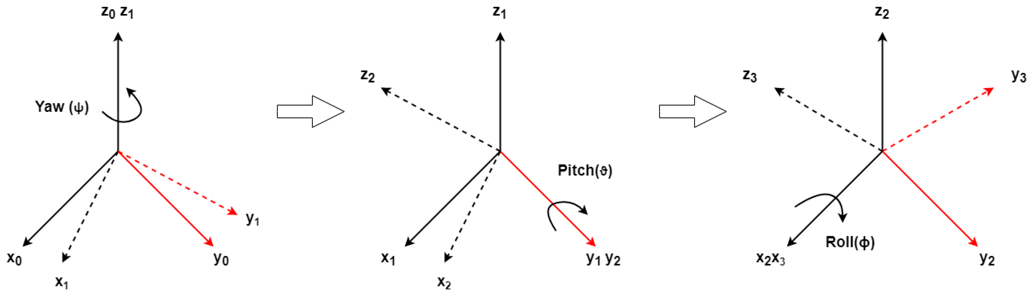
2.2. Transformation between Frames

To explain the kinematics of the symmetrical UAV quadrotor, it is necessary to understand the transition between the inertial frame and the body frame. The transition between frames may be represented by a set of rotations. The rotation matrices are used to transform any point from the inertial frame to the body frame. The rotation matrix can easily be explained by the vector projections of each axis as follows:

$$R=\left[\begin{array}{ccc}{x}_{\mathbf{1}}·x_{\mathbf{0}}& y_1·x_{\mathbf{0}}& z_1·x_{\mathbf{0}}\\ x_1·y_{\mathbf{0}}& y_1·y_{\mathbf{0}}& z_1·y_{\mathbf{0}}\\ x_{\mathbf{1}}·z_{\mathbf{0}}& y_1·z_{\mathbf{0}}& z_1·z_{\mathbf{0}}\end{array}\right]$$

(4)

Table 2. Vector projection.

$x_1·x_0=\cos \left(\mathsf{\psi }\right)$	$y_1·x_0=-\sin \left(\mathsf{\psi }\right)$	$z_1·x_0=0$
$x_1·y_0=\sin \left(\mathsf{\psi }\right)$	$y_1·y_0=\cos \left(\mathsf{\psi }\right)$	$z_1·y_0=0$
$x_1·z_0=0$	$y_1·y_0=0$	$z_1·z_0=1$

illustrates the vector projection of the symmetrical UAV quadrotor, and when considering the rotation about z-axis by angle ψ, as shown in Figure 1.

A set of rotations can represent a transformation between the inertial frame and body frame; thus, rotation matrices can be used to transform any point from the inertial frame to the body frame. The rotation matrix can easily be explained by the projections of each axis vector [18]. From the projections of the three vectors, the resultant rotational transformation matrix for the Roll-Pitch-Yaw representation “ZYX Euler angles” is as follows:

$$R_{Z,Y,X}=\left[\begin{array}{ccc}{C}_{\theta }{C}_{\psi }& C_{\psi }{S}_{\theta }{S}_{\varphi }-C_{\varphi }{S}_{\psi }& S_{\varphi }{S}_{\psi }+C_{\varphi }{C}_{\psi }{S}_{\theta }\\ C_{\theta }{C}_{\psi }& C_{\varphi }{C}_{\psi }+S_{\theta }{S}_{\varphi }{S}_{\psi }& C_{\varphi }{S}_{\theta }{S}_{\psi }-C_{\psi }{S}_{\varphi }\\ -S_{\theta }& C_{\theta }{S}_{\varphi }& C_{\theta }{C}_{\varphi }\end{array}\right]$$

(5)

Linear velocity in the inertial frame $\dot{\xi }={\left[\begin{array}{ccc}\dot{x}& \dot{y}& \dot{z}\end{array}\right]}^T$ is obtained by multiplying rotation matrix $R$ by the linear velocity of the quadrotor in the body frame $V_b={\left[\begin{array}{ccc}{u}_b& v_b& w_b\end{array}\right]}^T$. For linear velocity, the transformation matrix does not change with time. On the other hand, the angular velocity transformation matrix depends on time $w=\frac{d\theta }{dt}$. The derivation of the rotation matrix, such as the skew matrix, is used to determine the angular velocity vector. The rotation matrix can be derived as follows:

$$\dot{R}=\frac{dR}{dt}=\frac{dR}{d\theta }\frac{d\theta }{dt}=\dot{\theta }S\left(i\right)R\left(t\right)=S\left(\omega \left(t\right)\right)R\left(t\right)$$

(6)

where $S\left(\omega \left(t\right)\right)$ is the skew-symmetric for the angular velocity vector $\omega \left(t\right)$, $\omega \left(t\right)$ is the angular velocity vector of a rotating frame referenced to the fixed frame at time t, $\theta$ is the angle of rotation. Thus, the general rule is:

$$\dot{R_n^0}=S\left({\omega }_{0,n}^0\right)R_n^0$$

(7)

where ${\omega }_{0,n}^0$ links the current frame with the base frame and next frame. $R_n^0$ is the rotation matrix between frames,

$${\omega }_{0,3}^0={\omega }_{0,1}^0+R_1^0{\omega }_{1,2}^1+R_2^0{\omega }_{2,3}^2$$

(8)

For the quadrotor, three axes should be considered. Thus, three relative transformations are done to obtain the angular velocity vector,

$${\omega }_{0,3}^0=\left[\begin{array}{c}1\\ 0\\ 0\end{array}\right]\dot{\varphi }+\left[\begin{array}{c}0\\ cos\left(\varphi \right)\\ -sin\left(\varphi \right)\end{array}\right]\dot{\theta }+\left[\begin{array}{c}-sin\left(\theta \right)\\ cos\left(\theta \right)sin\left(\varphi \right)\\ cos\left(\varphi \right)cos\left(\theta \right)\end{array}\right]\dot{\psi }$$

(9)

The angular velocity vector of the quadrotor in body frame $\omega ={\left[\begin{array}{ccc}p& q& r\end{array}\right]}^{\mathrm{T}}$ is obtained by:

$$\left[\begin{array}{c}p\\ q\\ r\end{array}\right]=\left[\begin{array}{ccc}1& 0& -sin\left(\theta \right)\\ 0& cos\left(\varphi \right)& cos\left(\theta \right)sin\left(\varphi \right)\\ 0& -sin\left(\varphi \right)& cos\left(\varphi \right)cos\left(\theta \right)\end{array}\right] \left[\begin{array}{c}\dot{\varphi }\\ \dot{\theta }\\ \dot{\psi }\end{array}\right]$$

(10)

The angular velocity vector of the quadrotor in the inertial frame obtained by the inverse of the angular velocity matrix,

$$\left[\begin{array}{c}\dot{\varphi }\\ \dot{\theta }\\ \dot{\psi }\end{array}\right]=\left[\begin{array}{ccc}1& sin\left(\varphi \right)tan\left(\theta \right)& cos\left(\varphi \right)tan\left(\theta \right)\\ 0& cos\left(\varphi \right)& -sin\left(\varphi \right)\\ 0& sin\left(\varphi \right)/cos\left(\theta \right)& cos\left(\varphi \right)/cos\left(\theta \right)\end{array}\right]\left[\begin{array}{c}p\\ q\\ r\end{array}\right]$$

(11)

It can be seen that many forces affect the linear and rotational motion of multicopter. The most essential and effective forces as, gravitational force $F_g$, thrust force $F_t$ and aerodynamic drag force $F_d$ are considered in this research. It is assumed that the quadrotor is a rigid body, so all the forces produced by the rotors will have only one direction parallel to the z-axis of the body frame [19,20].

$$f_t=\sum _{i=1}^4{f}_i=k\sum _{i=1}^4{\omega }_i^2$$

(12)

where $f_i$ is the force generated by each rotor $i$ with an angular velocity ${\omega }_i$ along $z_b$ axis, k is the lift constant.

$$F_t=\left[\begin{array}{c}{S}_{\varphi }{S}_{\psi }+C_{\varphi }{C}_{\psi }{S}_{\theta }\\ C_{\varphi }{S}_{\theta }{S}_{\psi }-C_{\psi }{S}_{\varphi }\\ C_{\theta }{C}_{\varphi }\end{array}\right]f_t$$

(13)

$F_t$ represents the thrust force vector generated by the rotors mounted over the quadrotor.

$$F_d=\left[\begin{array}{c}{D}_x\\ D_y\\ D_z\end{array}\right]=\frac{1}{2}{\rho }_{air}I\left[\begin{array}{c}{A}_x\\ A_y\\ A_z\end{array}\right]\left[\begin{array}{ccc}{V}_x^2& 0& 0\\ 0& V_y^2& 0\\ 0& 0& V_z^2\end{array}\right]\left[\begin{array}{c}{C}_x\\ C_y\\ C_z\end{array}\right]$$

(14)

where $\rho$ is the density of air, $A_i$ is the cross-sectional area of the quadrotor exposed to wind, $V$ is the speed of quadrotor relative to wind speed, $C_f$ is the drag coefficient referenced to the inertial frame [21]. The total force vector affecting the motion of the quadrotor will be:

$$F=m\left[\begin{array}{c}\ddot{x}\\ \ddot{y}\\ \ddot{z}\end{array}\right]=\left[\begin{array}{c}0\\ 0\\ -mg\end{array}\right]+\left[\begin{array}{c}{S}_{\varphi }{S}_{\psi }+C_{\varphi }{C}_{\psi }{S}_{\theta }\\ C_{\varphi }{S}_{\theta }{S}_{\psi }-C_{\psi }{S}_{\varphi }\\ C_{\theta }{C}_{\varphi }\end{array}\right]f_t+\left[\begin{array}{c}{D}_x\\ D_y\\ D_z\end{array}\right]$$

(15)

The linear acceleration of the quadrotor body is obtained from the resultant force $F$,

$$\left[\begin{array}{c}{\ddot{x}}^b\\ {\ddot{y}}^b\\ {\ddot{z}}^b\end{array}\right]=\left[\begin{array}{c}\left(\left(S_{\varphi }{S}_{\psi }+C_{\varphi }{C}_{\psi }{S}_{\theta }\right)f_x+D_x\right)/m\\ \left(\left(C_{\varphi }{S}_{\theta }{S}_{\psi }-C_{\psi }{S}_{\varphi }\right)f_y+D_y\right)/m\\ \left(\left(\left(C_{\theta }{C}_{\varphi }\right)f_z+D_z\right)/m\right)-g\end{array}\right]$$

(16)

The rotational dynamics investigation is achieved by Euler–Lagrange and Newton–Euler methods. The Newton–Euler method sums all the forces that impact the quadrotor body [12,22]. The main Newton–Euler equation is given as:

$$\tau ={\rm I}\dot{v}+v x \left(Iv\right)+\Gamma$$

(17)

where $\tau$ is generated torques by rotors, ${\rm I}\dot{v}$ is the angular acceleration generated by the inertia of the quadrotor, $v x \left(Iv\right)$ are centripetal forces, $\mathsf{\Gamma }$ is gyroscopic forces. The total torque vector generated by rotors can be expressed as follows:

$$\left[\begin{array}{c}\begin{array}{c}\Sigma T\\ {\tau }_{\varphi }\end{array}\\ \begin{array}{c}{\tau }_{\theta }\\ {\tau }_{\psi }\end{array}\end{array}\right]=\left[\begin{array}{cccc}{c}_T& c_T& c_T& c_T\\ 0& l{c}_T& 0& -l{c}_T\\ -l{c}_T& 0& l{c}_T& 0\\ -c_Q& c_Q& -c_Q& c_Q\end{array}\right]\left[\begin{array}{c}{\omega }_1^2\\ {\omega }_2^2\\ {\omega }_3^2\\ {\omega }_4^2\end{array}\right]$$

(18)

where $c_T$ is the lumped variable of thrust factor proportion to the motor-prop system,$c_Q$ is torque factor for the motor-prop system, $l$ is the length of the quadrotor arm.

$$v x \left(Iv\right)=\left[\begin{array}{c}p\\ q\\ r\end{array}\right]x\left[\begin{array}{c}{I}_{xx}p\\ I_{yy}q\\ I_{zz}r\end{array}\right]$$

(19)

where $I_{xx}, I_{yy}$ and $I_{zz}$ represent the moment of inertia terms relative to the center of mass.

$$\mathsf{\Gamma }=I_r\left[\begin{array}{c}p\\ q\\ r\end{array}\right]x\left[\begin{array}{c}0\\ 0\\ 1\end{array}\right]{\omega }_{\mathsf{\Gamma }}$$

(20)

where $I_r$ is the moment of inertia for each rotor, ${\omega }_{\mathsf{\Gamma }}$ is the summation of the angular speed with respect to rotation direction, ${\omega }_{\mathsf{\Gamma }}={\omega }_1-{\omega }_2+{\omega }_3-{\omega }_4$. Thus, the angular acceleration will be as follows:

$$\dot{\mathsf{\upsilon }}=\left[\begin{array}{c}\dot{p}\\ \dot{q}\\ \dot{r}\end{array}\right]=\left[\begin{array}{c}\left(I_{yy}-I_{zz}\right)qr/I_{xx}\\ \left(I_{zz}-I_{xx}\right)pr/I_{yy}\\ \left(I_{xx}-I_{yy}\right)pq/I_{zz}\end{array}\right]-I_r\left[\begin{array}{c}q/I_{xx}\\ -p/I_{yy}\\ 0\end{array}\right]{\omega }_{\mathsf{\Gamma }}+\left[\begin{array}{c}{\tau }_{\varphi }/I_{xx}\\ {\tau }_{\theta }/I_{yy}\\ {\tau }_{\psi }/I_{zz}\end{array}\right]$$

(21)

The resultant equation of angular acceleration in the body frame can be transformed from the body frame to the inertial frame by finding the inverse of the above equations as follows:

$$\ddot{\eta }=\left[\begin{array}{ccc}0& \dot{\varphi }{C}_{\varphi }{T}_{\theta }+\frac{\dot{\theta }{S}_{\varphi }}{C_{\theta }^2}& -\dot{\varphi }{S}_{\varphi }{C}_{\theta }+\frac{\dot{\theta }{C}_{\varphi }}{C_{\theta }^2}\\ 0& -\dot{\varphi }{S}_{\varphi }& -\dot{\varphi }{C}_{\varphi }\\ 0& \frac{\dot{\varphi }{C}_{\varphi }}{C_{\theta }}+\frac{\dot{\varphi }{S}_{\varphi }{T}_{\theta }}{C_{\theta }}& -\frac{\dot{\varphi }{S}_{\varphi }}{C_{\theta }}+\frac{\dot{\theta }{C}_{\varphi }{T}_{\theta }}{C_{\theta }}\end{array}\right]\left[\begin{array}{c}p\\ q\\ r\end{array}\right]+W_{\eta }^{-1}\left[\begin{array}{c}\dot{p}\\ \dot{q}\\ \dot{r}\end{array}\right]$$

(22)

The linear and angular acceleration vector of the system will be as follows:

$${\left[\begin{array}{cc}\ddot{\xi }& \ddot{\eta }\end{array}\right]}^T={\left[\begin{array}{cccccc}\ddot{x}& \ddot{y}& \ddot{z}& \ddot{\varphi }& \ddot{\theta }& \ddot{\psi }\end{array}\right]}^T$$

(23)

From this vector, we can derive angular acceleration vector, linear acceleration vector, angular position vector and linear position vector. At this point, the modeling of the quadrotor is completed, and we can now design our controller. Some modifications were carried out to transform IFR and NIFR. Generally, velocity expressed in the body frame is multiplied with a rotation matrix to obtain an acceleration of the UAV quadrotor expressed in IFR as follows:

$$\left[\begin{array}{c}{\dot{x}}_b^i\\ {\dot{y}}_b^i\\ {\dot{z}}_b^i\end{array}\right]=R\left[\begin{array}{c}{u}_b\\ v_b\\ w_b\end{array}\right]$$

(24)

The relation between the quadrotor body frame and the vessel moving frame can be obtained in two steps: First, by considering the relation between the body frame and IFR, second, by considering the relation between the moving frame and IFR, which is followed by combining them as:

$${\dot{\xi }}_b^m={\dot{\xi }}_b^i-{\dot{\xi }}_m^i=\left[\begin{array}{c}{\dot{x}}_b^i\\ {\dot{y}}_b^i\\ {\dot{z}}_b^i\end{array}\right]-\left[\begin{array}{c}{\dot{x}}_m^i\\ {\dot{y}}_m^i\\ {\dot{z}}_m^i\end{array}\right]=\left[\begin{array}{c}{\dot{x}}_b^m\\ {\dot{y}}_b^m\\ {\dot{z}}_b^m\end{array}\right]$$

(25)

$$Velocityerror={\dot{\xi }}_{desired}^m-{\dot{\xi }}_b^m$$

(26)

where ${\dot{\xi }}_b^i$ is the position state vector of the body frame related to IFR, ${\dot{\xi }}_m^i$ is the position state vector of the moving frame related to IRF, while ${\dot{\xi }}_b^m$ is the resultant position state vector. Usually, the state feedback vector of position, velocity, angular position and angular velocity relation to IRF is expressed as follows:

$$\dot{x}={\left[x y z u v w \varphi \theta \psi p q r\right]}^T$$

(27)

In the case of NIFR, the state of position and velocity of the moving frame should be included in the state feedback vector,

$$\dot{x}={\left[\begin{array}{ccccccccc}{x}_b& y_b& z_b& u_b& v_b& w_b& x_m& y_m& z_m\\ u_m& v_m& w_m& \varphi & \theta & \psi & p& q& r\end{array}\right]}^T$$

(28)

The error of position vector in the body frame is a combination of referencing the position feedback state of the body frame with position feedback state of the moving frame as given below,

$$x_{err}^b=x_d^m+x_m^i-x_b^i$$

(29)

where $x_d^m$ is the desired position in the x-axis referenced to the moving frame (NIFR), $x_m^i$ is position state of the moving frame, $x_b^i$ is the position state of the body frame referenced to the inertial frame. The same procedure is used for the y-axis and z-axis.

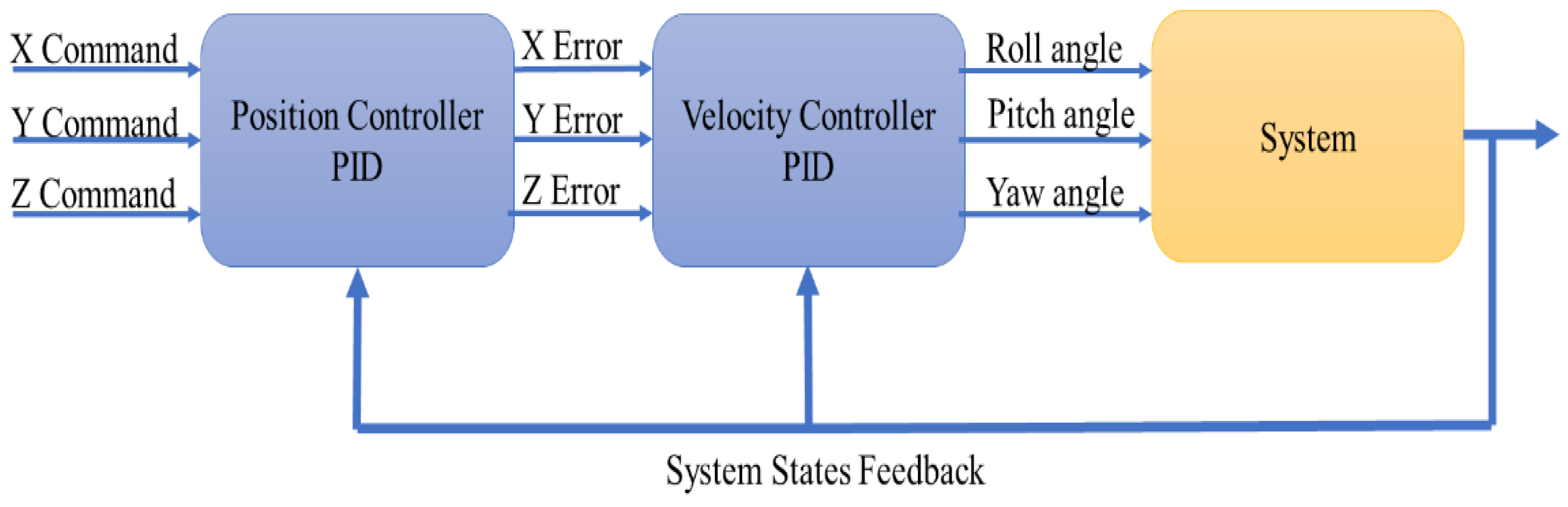
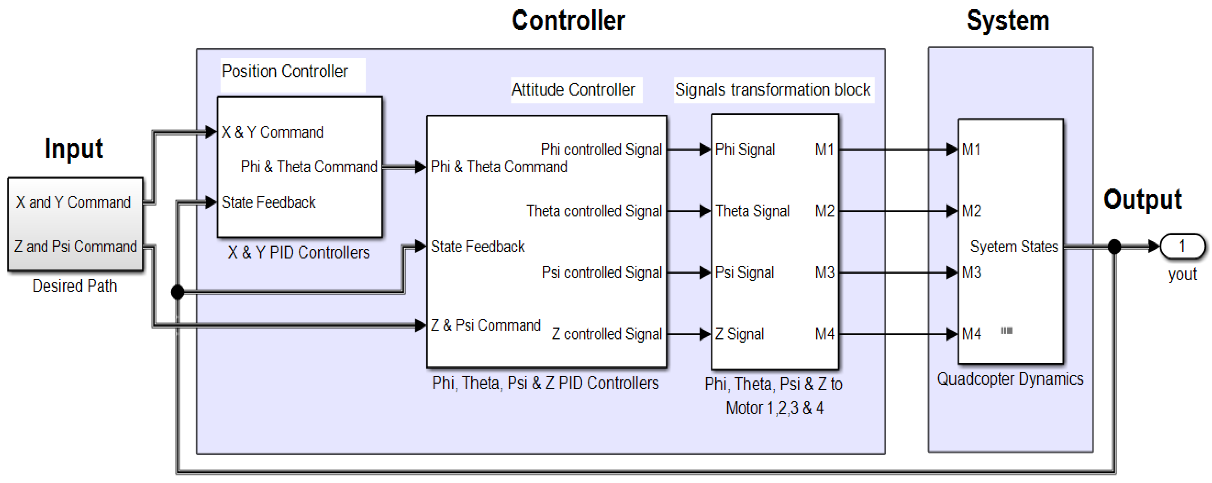
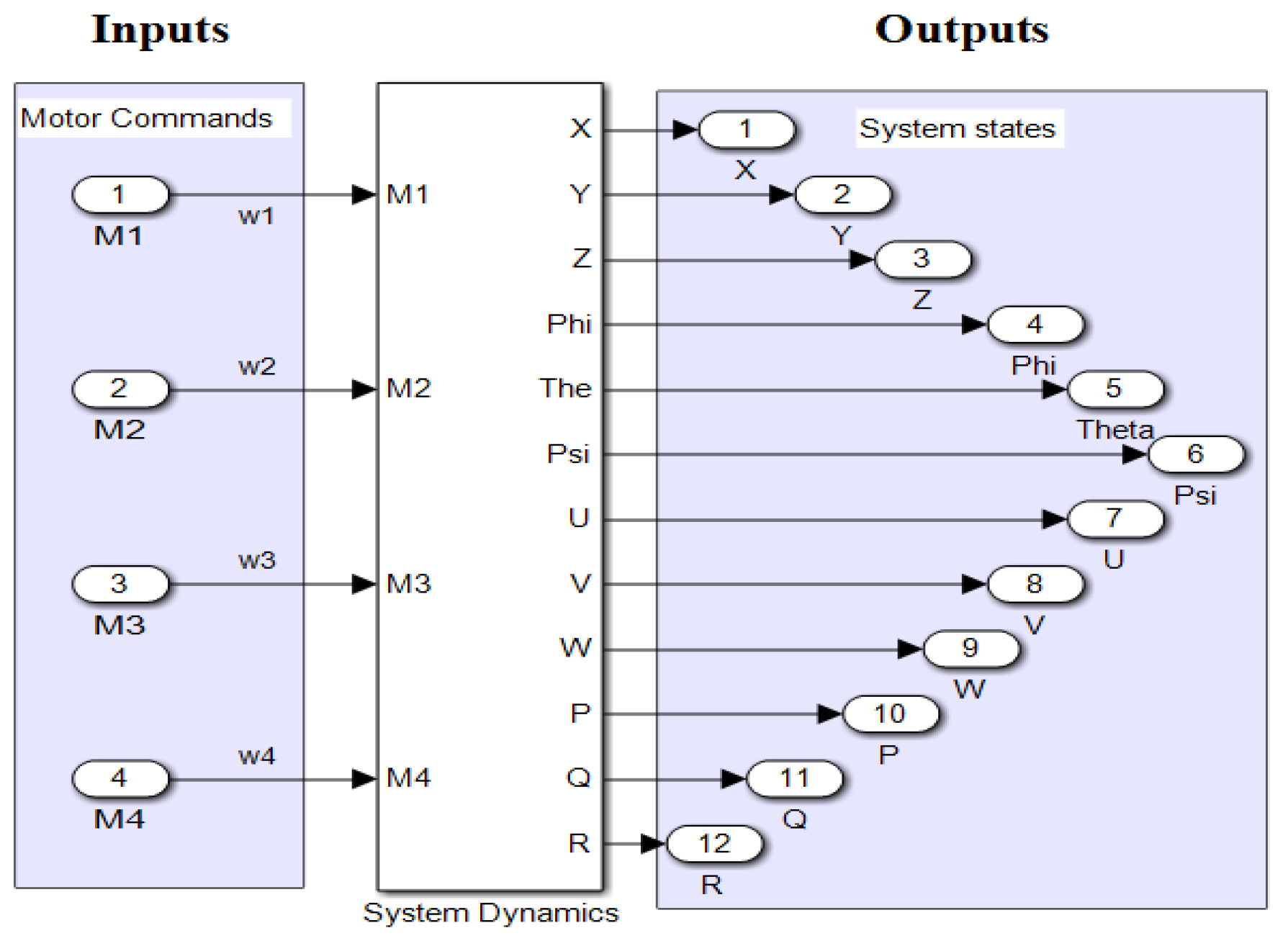
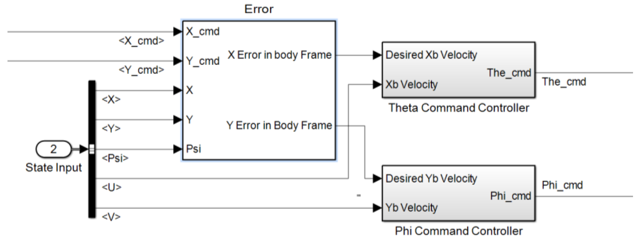
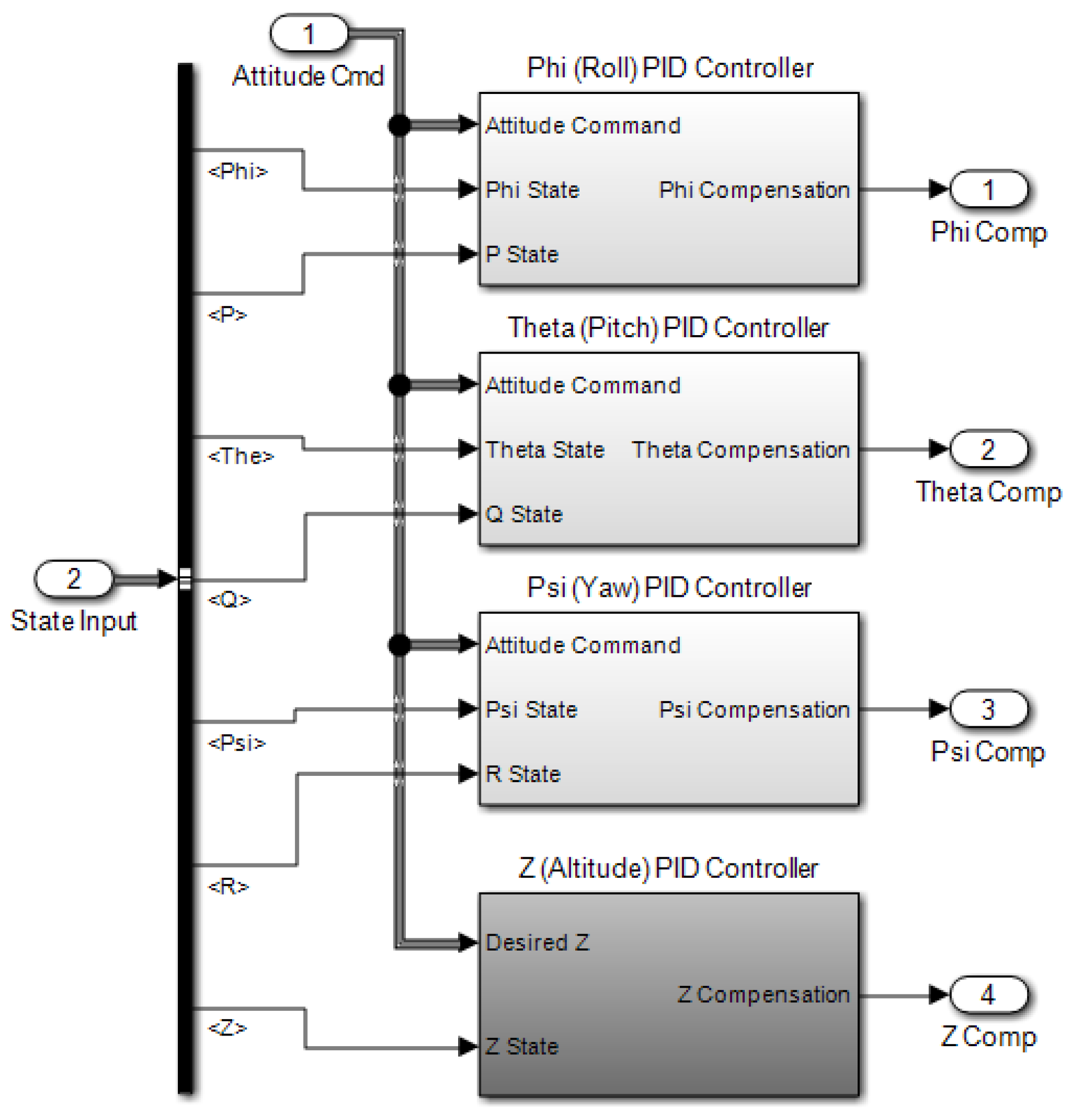
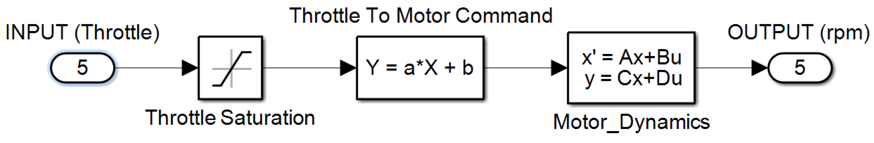
3. Multi-Stage PID Controller

In this study, it is proposed to use a PID controller for the control of the quadrotor. The PID controller is chosen as it will provide the desired stability with minimum mathematical calculations. The simplicity of the controller is important due to the limitation of processor, memory and physical microcontroller specifications. The mathematical formulation of the PID is expressed in the s-domain as follows:

$$u\left(t\right)=K_{p}e\left(t\right)+K_i\int e\left(t\right)dt+K_d\frac{de\left(t\right)}{dt}$$

(30)

The main assumption in this study is to take a signal from a specific path as command input to the system. The path provides the information of the X, Y and Z position in time-series as an input to the system; also, the path command provides the required Psi angle of the quadrotor. The Phi and Roll angle commands are passed after processing the X and Y command. The overall structure of the system and controller is given in Figure 2. The system block of Figure 3 contains symmetrical UAV dynamics. In the previous section, the dynamics of the system were explained; the system block is considered as a black box with inputs and outputs. The block system inputs are angular velocities of the rotors (w_1, w_2, w_3, w_4), the outputs of the block system are the states of the system and contains the symmetrical UAV velocity vector (u, v, w), the angular velocity vector (p, q, r), position vector (x, y, z), and angular position vector (φ, θ, ψ), as shown in Figure 4. The controller consists of three stages; the first stage is the X and Y position controller. The second stage is the altitude controller to control the Phi, Theta, Psi and Z commands. The third stage is the translation from Phi, Theta, Psi, and the altitude correction signals to a throttle signal as an input to four rotors. The first stage controller inputs are the X, Y and Psi angle commands where X and Y are feedback states, and U and V are the velocities as the change of position feedback. The outputs are the Phi and Theta angles commands, as shown in Figure 5. The representation of position error in the inertial frame is expressed as:

$$x_{err}^i=x_{cmd}^i-x_{state}^i$$

(31)

$$y_{err}^i=y_{cmd}^i-y_{state}^i$$

(32)

The error signal is multiplied with the rotation matrix to transform the error signal from the inertial frame to the body frame.

$$x_{err}^b=x_{err}^i\cos \left(\psi \right)+y_{err}^i\sin \left(\psi \right)$$

(33)

$$y_{err}^b=y_{err}^i\cos \left(\psi \right)-y_{err}^i\sin \left(\psi \right)$$

(34)

The x and y errors represented in the body frame will be transformed as a velocity signal in the desired axis to overcome the error in that axis,

$$u_{desired}^b=x_{err}^b$$

(35)

$$v_{desired}^b=y_{err}^b$$

(36)

The velocity error will be the difference between the desired velocity $u_{desired}^b$ in the x-axis and the state feedback velocity $u_{state}^b$. The output of the controller will be the angle command ${\theta }_{cmd}$. The maximum and minimum angle of inclination “bank angle” should be considered to avoid losing control during flight.

$${\theta }_{cmd}=\{\begin{array}{cc}-{12}^o,\hfill & \theta \le -{12}^o\\ K_p\left(U_{desired}^b-U_{state}^b\right)-K_d{U}_{state}^b,\hfill & -{12}^o<\theta <{12}^o\\ 12,\hfill & \theta \ge {12}^o\end{array}$$

(37)

Of course, the bank angle varies from one application to another; even some quadrotors are designed for acrobatic flights and sports competitions. In such cases, the bank angle will be unlimited. The same procedure is followed to obtain ${\phi }_{cmd}$.

Initially, all six controllers were PID controllers, but during the optimization process with AGA, the controller of the $x$ and $y$ axes changed to PD controller. Hence, the optimization process sets the integral parameter for the $x$ and $y$ axes controllers to zero. In this case, the PD controller provided better performance than PID.

The inputs to the second stage controller are ${\phi }_{cmd}$, ${\theta }_{cmd}$, ${\psi }_{cmd}$ and $z_{cmd}$ command signals, ${\phi }_{state}$, ${\theta }_{state}$, ${\psi }_{state}$, $P_{state}$, $Q_{state}$ and $R_{state}$ are feedback states to the controller. For example, the controller compensates the angle commands and altitude (z) command as a correction signal. The controller structure is given in Figure 6. The mathematical formula of the second stage controller is given below, the same formula for $\phi$, $\psi$, and z:

$${\theta }_{Comp}\left(t\right)=K_p\left({\theta }_{cmd}\left(t\right)-{\theta }_{state}\left(t\right)\right)+K_i\int \left({\theta }_{cmd}\left(t\right)-{\theta }_{state}\left(t\right)\right)dt+K_d\ast Q_{state}\left(t\right)$$

(38)

The second stage’s output will be an input to the third stage; in this part, the controller will translate the compensation values to the throttle command “Rotors command”. The throttle signal $T{h}_i$ of each rotor, $i$ can be given by:

$$\left[\begin{array}{c}T{h}_1\\ T{h}_2\\ T{h}_3\\ T{h}_4\end{array}\right]=\left[\begin{array}{cccc}1& -1& -1& -1\\ 1& 1& -1& 1\\ 1& 1& -1& -1\\ 1& -1& 1& 1\end{array}\right]\left[\begin{array}{c}{Z}_{comp}\\ {\phi }_{comp}\\ {\theta }_{comp}\\ {\psi }_{comp}\end{array}\right]$$

(39)

$$M_{cmd}^i=\{\begin{array}{cc}0,\hfill & T{h}_i\le T{h}_{min}\\ a\ast T{h}_i+b,\hfill & T{h}_{min}<T{h}_i<T{h}_{max}\\ a\ast T{h}_{max}+b,\hfill & T{h}_i\ge T{h}_{max}\end{array}$$

(40)

where $a$ and $b$ are constants and obtained from the motor specification, the motor command is considered as an input to the motor’s dynamics system block. The output is the rotor angular velocity given in a revolutions per minute (rpm) signal; the motor block system is shown in Figure 7.

4. Genetic Algorithm

GA generally follows these steps: genetic representation, initial population, fitness function, genetic operations. For genetic representation, every gene/individual represents a PID parameter in decimal number format, each PID controller contains 3 genes represented as $K_p$, $K_i$ and $K_d$ values. Thus, we have 6 PID controllers for $\left(x, y, z, \phi , \theta ,\psi \right)$, one chromosome consists of 18 genes.

The adaptive GA only differs from the conventional GA in the way it generates the new population. In conventional GAs, generating a new population consists of selecting parents and the crossover process. However, the proposed adaptive GA method divides the generation process into three steps:

(1)

The solutions are tested, then they are sorted as such that the first chromosome is the best solution, then the second solution is the second chromosome, and so on. The selection process is then accomplished by choosing the best half of the sorted population. The best-sorted half of the population will be the new parent chromosomes. Then, using the crossover process, 50% of the new population is generated.

(2)

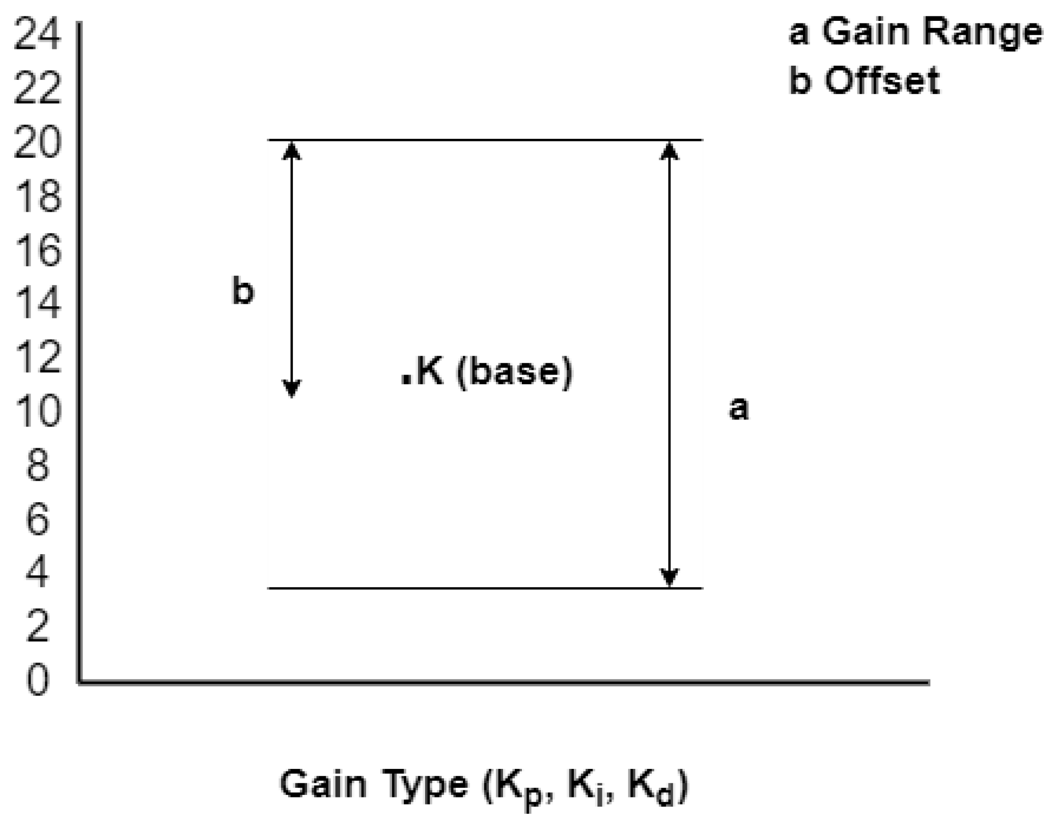
Generated constrained random solutions are around one-third of the best-sorted solutions of the random gain range value (the gain range is very small), see Figure 8; 30% of the new population is generated using this method.

(3)

Generated constrained random solutions are around one-fifth of the best-sorted solutions of the old population. The main difference between this step and the previous step is the use of a wider gain range of a random value. The aim of this step is to avoid falling into the local minimum solution. This step can be considered as a mutation to refresh the optimization process.

Using decimal numbers format makes generating an initial constrained population easier, and it will help to generate new constrained random chromosomes. The base values of the PID parameters were taken from a previous study [13], and then a constrained random function with different weights generated 100 chromosomes close to the base values of the initial population. New chromosomes are generated by summing individual genes with a random constraint weight. The formula for generating the initial random population is given below:

$$k_m^n\left(l\right)=k_m^n\left(base\right)+\left(R\ast a_m^n-b_m^n\right)$$

(41)

where $k$ is the gain parameter, $m$ is gain type $\left\{\mathrm{P},\mathrm{I}, and \mathrm{D}\right\}$, n is the axis or angle $\left\{x,y,z,\phi ,\theta , \psi \right\}$, $l$ is the number of the chromosome in the initial population, $R$ is a random number between zero and one, a is the width of random values, b is the offset of random values. Limiting gain values prevents the system from entering an unstable region. It can prevent MATLAB from running the process normally—it can cause an infinite processing loop if it happens. The fitness function can be the sum of squared error, absolute error, squared time-weighted error, or a mix of other functions. In this study, the sum of squared error and max of squared error was used. The fitness function was constructed as a sum of squared error for each PID controller, the maximum error for each PID controller, and the sum of squared error for all PID controllers’ results. Each term is multiplied by a weight value and these weight values can be changed by the user depending on the response and performance of AGA operations. The overall fitness value (FV) will be as follows:

$$Fitnessvalue=w_1\ast {{\displaystyle \int }}_0^{\infty }{e}_{total}^2\left(t\right)dt+{\displaystyle \sum }_i^6(w_2\ast {{\displaystyle \int }}_0^{\infty }{e}_i^2\left(t\right)dt+w_3\ast max$$

(42)

where $i$ represents PID source, $i=\left\{x,y,z,\phi ,\theta ,\psi \right\}$, $e_i$ represents an error of each PID controller, $e_{total}$ represents the total error of all PID controllers. Each chromosome will be evaluated depending on its fitness value. Then, the chromosomes are sorted; thus, the best chromosome “solution” is the first chromosome in the population.

Adaptive GA advantages can be summarized as follows.

• It uses a small number of chromosomes within the population, resulting in a minimized processing time for each iteration;
• Adaptive PID gains values for an improved control system, as shown in Equation (41);
• It improves performance by avoiding falling in the local minimum by widening the range of the gains for 20% of a new generation;
• Each iteration gains range change is based on the best solution.

5. Simulation and Results

For the simulation, the symmetrical UAV quadrotor specifications are based on actual measurements carried out by a previous study [13]. The symmetrical UAV (quadcopter) weight is about 1 kg with a diameter of 44 cm. The results of the multi-stage controller are obtained by employing a random path to obtain the desired coordinates $\left(x,y,z,\psi \right)$, and the coordinates are given as a time-series signal. The signal is used as an input to the multicopter system. In this study, the path is not symmetrical. This will be useful if an offline optimization for specific paths is to be performed. In this study, the path is not symmetric. Therefore, it is imperative to conduct offline optimization for a specific path. The simulation steps are shown in

Table 3. Desired path represented in time-series.

Steps	Time (Seconds)	x-Axis (Meter)	y-Axis (Meter)	z-Axis (Meter)	Psi Angle (Degree)
1	0	0	0	3	0
2	5	0	0	3	0
3	10	20	0	3	0
4	15	20	5	3	0
5	20	40	5	3	0
6	25	60	5	3	0
7	30	80	10	3	0

, and the time-series function in MATLAB gives a smooth and gradual transition between steps.

The integral square error of both the conventional GA and the adaptive GA is given in

Table 4. Comparison of ISE between GA and AGA.

Number	Conventional GA ISE	Adaptive GA ISE
1	395,87	395,87
2	397,198	363,929
3	388,363	354,026
4	384,874	337,825
5	384,803	318,168
6	384,490	310,480
7	384,106	314,313
8	384,106	307,316
9	381,619	290,028
10	381,625	386,261

.

A comparison between the desired path and simulated path was carried out before and after AGA optimization. Figure 9 shows the results in 2D for the $x$ and $y$ axes. The unoptimized results show that the symmetrical UAV quadrotor missed the path after a sharp turning by 1.77 m before recovering and following the correct path. However, the genetically optimized quadrotor results missed the path by only 0.76 m. The results also show that the symmetrical UAV quadrotor’s optimization process to recover and return to the desired position is much faster, and is with better performance and less power consumption. Meaning, that the optimization has significantly improved the response, which positively affected the command and the results of both Phi and Theta angles, as shown in Figure 10 and Figure 11, thus resulting in an improvement in the stability of the system.

Figure 12 shows the step response on the z-axis. It can be seen that the optimizations significantly improved the overshoot and transient response as well as the overall performance and power consumption.

The close to zero overshoot result is due to a take-off command signal. This is simulated as a sharp step signal over the z-axis without any movement in other directions; optimizing this movement can be considered easier than others since the activity is on a single axis. However, the next steps also affect the altitude, but fast recovery is achieved due to the controller robustness. The enhanced performance results were made possible by optimizing all the PID controller parameters in parallel.

The output of the y-axis controller improves the Phi angle command. Figure 10 shows the controller commands and responses for the Phi angle. The sample interval between 15 and 17 s of flight simulation shows the differences between the command signals and response signals before and after AGA optimization. In this interval, to reach the desired position, the controller gave a command to the Phi angle to turn by 6.6 degrees; however, AGA optimization reduced the command signal by about 30% to 4.8 degrees. Thus, the symmetrical UAV quadrotor reaches the desired position with a smaller Phi angle, which means more stability and less power consumption. The maximum delay between the command and control signal before AGA optimization is 0.6 s; in some cases, this delay can affect the stability, but after AGA optimization, the maximum delay between the command and control signal becomes 0.14 s, which means a 75% improvement.

Figure 11 shows a scoped interval to study the characteristics of commands and response signals. At the fifth second of flight simulation, a sharp step command was given by the x-axis controller, trying to follow the desired position. The command signal reached its predefined limit by 12 degrees; this action is shown as a step input on the Theta angle; this action will aid in the system characteristics investigation. AGA improved the rising time off $t_r=0.84\mathrm{s}$ achieved by conventional GA down to $t_r=0.28\mathrm{s}$. The optimization improved the response time of the system, plus a clear overshot improvement from PO = 18.5% down to 5.25. The Psi angle command is zero; however, it is greatly affected by the activities of other controller responses and actions.

The effect, as shown in Figure 13, is an oscillatory one that increases with time. Since the oscillation amplitude increases, it can be seen that it will reach instability at some point. Figure 12 shows the AGA optimization improved the controller’s ability to deal with the oscillation. The results show that the optimized Psi angle controller fully recovers after each side effect caused by the actions of other controllers.

The total thrust consumed during the test flight was $1.26\times {10}^5$; however, the total thrust consumed for the same flight employing the optimized controllers was $1.05\times {10}^5$. This is a clear indication that the AGA optimization introduced a 16.2% thrust consumption improvement. To evaluate the efficiency of the proposed adaptive GA optimization method a full test was carried out using a conventional GA to optimize the controllers. This was then compared with the results [5] obtained using the AGA optimized controllers. In both tests, a population of 100 was used with 100 chromosomes in the initial population. The results were recorded for 10 iteration runs. In both cases, the evaluation is based on the MSE for all the PID controllers.

6. Conclusions

In this study, complete modeling of a nonlinear 6-DOF symmetrical UAV quadrotor system was introduced and included the relationship between the body frame of the symmetrical UAV quadrotor and the non-inertial frame of reference. A multi-stage PID controller was designed and used to control the quadrotor system. An adaptive genetic algorithm was developed and used to optimize the performance of multi-stage PID controllers. Optimizing multi-stage PID controllers with an adaptive genetic algorithm improved the quadrotor system’s performance and power consumption. The AGA had an added advantage over the conventional GAs; the AGA is guaranteed to avoid falling into local minima. It also required fewer iterations to achieve highly improved optimization results. From the results, it can be concluded that the use of the optimized multi-stage PID controller improved the system’s overall performance. The results showed that the proposed system outperformed the performance achieved by previous studies for similar system specifications.

References

1. Turkoglu, K.; Ozdemir, U.; Nikbay, M.; Jafarov, E. PID parameter optimization of a UAV longitudinal Flight control system. World Acad. Sci. Eng. Technol. 2008, 45, 340–345. [Google Scholar]
2. Turkoglu, K.; Jafarov, E.M. Hinf loop shaping robust control vs. classical PI(D) control: A case study on the longitudinal dynamics of hezarfen UAV. In Proceedings of the 2nd WSEAS International Conference on Dynamical Systems and Control, Bucharest, Romania, 16–17 October 2006; pp. 105–110. [Google Scholar]
3. Dawes, J.; Ng, L.; Dorf, R.; Tam, C. Design of Deadbeat Robust Systems. In Proceedings of the IEEE International Conference on Control and Applications, Glasgow, UK, 24–26 August 1994; pp. 1597–1598. [Google Scholar]
4. Lockheed Martin. Kestrel Autopilot System: User Guide, Copyright© 2004–2008; Procerus® Technologies: Orem, UT, USA, 2015. [Google Scholar]
5. Kumar, P.V.; Challa, A.; Ashok, J.; Narayanan, G.L. GIS based fire rescue system for industries using Quad copter—A novel approach. In Proceedings of the International Conference on Microwave, Optical and Communication Engineering (ICMOCE), Bhubaneswar, India, 18–20 December 2015; pp. 72–75. [Google Scholar] [CrossRef]
6. Dallal Bashi, O.I.; Wan Hasan, W.Z.; Azis, N.; Shafie, S.; Wagatsuma, H. Quadcopter sensing system for risky area. In Proceedings of the IEEE Regional Symposium on Micro and Nanoelectronics (RSM), Batu Ferringhi, Malaysia, 23–25 August 2017; pp. 216–219. [Google Scholar] [CrossRef]
7. Saha, H.; Basu, S.; Auddy, S.; Dey, R.; Nandy, A.; Pal, D.; Roy, N.; Jasu, S.; Saha, A.; Chattopadhyay, S.; et al. A low cost fully autonomous GPS (Global Positioning System) based quad copter for disaster management. In Proceedings of the 8th Annual Computing and Communication Workshop and Conference (CCWC), Las Vegas, NV, USA, 8–10 January 2018; pp. 654–660. [Google Scholar] [CrossRef]
8. Zhang, X.; Li, X.; Wang, K.; Lu, Y. A Survey of Modelling and Identification of Quadrotor Robot. Abstr. Appl. Anal. 2014, 2014, 320526. [Google Scholar] [CrossRef]
9. Chovancová, A.; Fico, T.; Chovanec, Ľ.; Hubinsk, P. Mathematical Modelling and Parameter Identification of Quadrotor (a survey). Procedia Eng. 2014, 96, 172–181. [Google Scholar] [CrossRef] [Green Version]
10. Bouabdallah, S.; Noth, A.; Siegwart, R. PID vs LQ control techniques applied to an indoor micro quadrotor. In Proceedings of the IEEE/RSJ International Conference on Intelligent Robots and Systems (IROS) (IEEE Cat. No. 04CH37566), Sendai, Japan, 28 September–2 October 2004; Volume 3, pp. 2451–2456. [Google Scholar] [CrossRef] [Green Version]
11. Khuwaja, K.; Tarca, I.C.; Tarca, R.C. PID Controller Tuning Optimization with Genetic Algorithms for a Quadcopter. Recent Innov. Mech. 2018, 5, 1–7. [Google Scholar] [CrossRef]
12. Luukkonen, T. Modeling and Control of Quadcopter. Independent Research Project in Applied Mathematics; Aalto University: Espoo, Finland, 2011; Available online: https://sal.aalto.fi/publications/pdf-files/eluu11_public.pdf (accessed on 23 September 2021).
13. Hemingway, E.G.; O’Reilly, O.M. Perspectives on Euler angle singularities, gimbal lock, and the orthogonality of applied forces and applied moments. Multibody Syst. Dyn. 2018, 44, 31–56. [Google Scholar] [CrossRef]
14. Mascarello, L.N.; Quagliotti, F. Analysis of Safety Requirements for Small Unmanned Aerial Systems (sUAS). In Handbook of Unmanned Aerial Vehicles; Valavanis, K., Vachtsevanos, G., Eds.; Springer: Cham, Switzerland, 2018. [Google Scholar] [CrossRef]
15. Cai, G.; Chen, B.M.; Lee, T.H. Unmanned Rotorcraft Systems. In Advances in Industrial Control; Springer: Singapore, 2011. [Google Scholar] [CrossRef]
16. Najm, A.A.; Ibraheem, I.K. Nonlinear PID controller design for a 6-DOF UAV quadrotor system. Eng. Sci. Technol. Int. J. 2019, 22, 1087–1097. [Google Scholar] [CrossRef]
17. David, H. Quadcopter Dynamic Modeling and Simulation for Control System Design; Drexel University: Philadelphia, PA, USA, 2014; Available online: www.mathworks.com/academia/student-challenge/spring-2014.html (accessed on 25 September 2021).
18. Spong, M.W.; Hutchinson, S.; Vidyasagar, M. Robot Modeling and Control. Ind. Robot. 2006, 33, 403. [Google Scholar] [CrossRef] [Green Version]
19. Musa, S. Techniques for Quadcopter Modelling & Design: A review. J. Unmanned Syst. Technol. 2017, 5, 66–75. Available online: http://www.ojs.unsysdigital.com/index.php/just/article/view/10.21535%252Fjust.v5i3.981 (accessed on 27 September 2021).
20. Cano, J.M. Quadrotor UAV for Wind Profile Characterization. Master’s Thesis, Universidad Carlos III de Madrid, Madrid, Spain, 2013. Available online: https://e-archivo.uc3m.es/bitstream/handle/10016/18105/PFC_Javier_Moyano_Cano.pdf?isAllowed=y&sequence=1 (accessed on 28 September 2021).
21. Dikmen, I.C.; Arisoy, A.; Temeltas, H. Attitude control of a quadrotor. In Proceedings of the 2009 4th International Conference on Recent Advances in Space Technologies, Istanbul, Turkey, 11–13 June 2009. [Google Scholar]
22. Artale, V.; Milazzo, C.; Ricciardello, A. Mathematical modeling of hexacopter. Appl. Math. Sci. 2013, 7, 4805–4811. [Google Scholar] [CrossRef]
Figure 1. Roll-Pitch-Yaw rotations.
Symmetry 14 00689 g001
Figure 2. Block diagram of multi-stage PID control system.
Symmetry 14 00689 g002
Figure 3. Symmetrical UAV (quadrotor) system and controller structure.
Symmetry 14 00689 g003
Figure 4. System dynamics block inputs and outputs.
Symmetry 14 00689 g004
Figure 5. The structure of the first stage PD controller.
Symmetry 14 00689 g005
Figure 6. The structure of the second stage PID controller.
Symmetry 14 00689 g006
Figure 7. The structure of motor controller and system.
Symmetry 14 00689 g007
Figure 8. PID random values constraints.
Symmetry 14 00689 g008
Figure 9. The flight path is on the x-axis and y-axis.
Symmetry 14 00689 g009
Figure 10. Result of Phi angle commands and responses.
Symmetry 14 00689 g010
Figure 11. Result of Phi angle commands and responses.
Symmetry 14 00689 g011
Figure 12. Controller response on the z-axis.
Symmetry 14 00689 g012
Figure 13. Result of Phi angle commands and responses.
Symmetry 14 00689 g013