Exploration of Temperature Distribution through a Longitudinal Rectangular Fin with Linear and Exponential Temperature-Dependent Thermal Conductivity Using DTM-Pade Approximant

Abstract

The present study elaborates on the thermal distribution and efficiency of a longitudinal rectangular fin with exponentially varying temperature-dependent thermal conductivity and heat transfer coefficient concerning internal heat generation. Also, the thermal distribution of a fin is comparatively studied for both exponentially varying temperature-dependent thermal conductivity and linearly varying temperature-dependent thermal conductivity. Further, the thermal distribution of a longitudinal fin is examined by using ANSYS software with different fin materials. Many physical mechanisms can be explained by ordinary differential equations (ODEs) with symmetrical behavior, the significance of which varies based on the perspective. The governing equation of the considered problem is reduced to a non-linear ODE with the assistance of dimensionless terms. The resultant equation is solved analytically using the DTM-Pade approximant and is also solved numerically using Runge-Kutta Fehlberg’s fourth-fifth (RKF-45) order method. The features of dimensionless parameters influencing the fin efficiency and temperature profile are discussed through graphical representation for exponentially and linearly varying temperature-dependent thermal conductivity. This study ensures that the temperature field enhances for the higher magnitude of thermal conductivity parameter, whereas it diminishes for diverse values of the thermo-geometric parameter. Also, greater values of heat generation and heat transfer parameters enhance the temperature profile. Highlight: Thermal distribution through a rectangular profiled straight fin is examined. Linear and non-linear thermal properties are considered. The combined impact of conduction, convection, and internal heat generation is taken for modeling the energy equation of the fin. Thermal simulation is performed for Aluminum Alloy 6061 (AA 6061) and Cast Iron using ANSYS.

1. Introduction

The heat transfer process is significant when the temperature of different bodies or parts of the same body varies. Convection of fluids, conduction in solids, and radiation are the three modes of heat transfer. A higher heat transfer rate is generally essential in industrial manufacturing processes. Traditional heat transfer methods are ineffective in generating the essential heat transfer rate for industrial applications. The use of cooling fluid, nanofluid, and hybrid nanofluids in the industrial sector is one of the techniques for achieving a high heat transfer rate. Numerous investigations explained the role of these kinds of liquids in the heat transfer process [1,2,3,4,5,6,7]. Usage of extended surfaces in various mechanical and engineering applications seems to be another approach to enhance heat transfer rate. Extended surfaces or fins are frequently used in various engineering systems to expand the heat transference area, dissipate heat generated inside the system, and extend the system’s functioning. Fins are used in oil-carrying pipelines, computer processor cooling, air conditioning, refrigeration, and air-cooled craft engines. Fins also play a prominent role in solidification augmentation in the energy storage system [8,9]. Fins are divided into longitudinal, radial, and pin fins. To improve heat dissipation from a heated main surface, a longitudinal fin of different profiles with a constant cross-sectional area is extensively utilized in practice. This fin is most effective when used in a natural convection setting with a low convection heat transfer coefficient. Motivated by these properties, several researchers examined the heat transfer properties of longitudinal fins with several influencing factors. Kundu [10] elaborated the comparative and unified research on the longitudinal fin and discussed the thermal analysis with optimal design. For a fin having a constant area with temperature variance, internal heat production, and thermal conductivity, Aziz and Bouaziz [11] derived the analytically approximate with very accurate solutions for temperature thermal distribution, fin efficiency, and optimal fin parameter. Najafabadi et al. [12] investigated analytical solutions for the non-linear differential equation (NLDE) model of a longitudinal fin with thermal conductivity and heat production. In the presence of internal heat generation, Sowmya et al. [13,14] conferred the thermal properties of longitudinal fin and moving rod owing to natural convection and radiation.

On the other hand, due to differences in thickness, the longitudinal fin has variable profiles depending on the shape. There are two techniques for solving fin optimization issues. The initial step in solving an optimization issue is to choose a basic profile (triangular or rectangular) and to calculate the fin dimensions. In reality, the rectangular profile is commonly utilized in the heat exchanger system due to its ease of production. As a result, additional research is being done to find the best size for these sorts. Recently, numerous researchers deliberated the heat transference analysis via different fins with rectangular profiles [15,16,17,18,19]. The study of fins for improving heat transmission has piqued the interest of many scholars during the last decade. When a fin’s cross-section is tiny, the temperature variation in the cross-section is correspondingly minimal. Then there is just a considerable temperature variation in the direction of the fin’s length. Put another way, the temperature distribution in the fin is a one-dimensional temperature field running parallel to the fin’s length. Several researchers explored thermal distribution analysis in past decades by considering different fins. Tarobi et al. [20] inspected the aspects of thermal distribution in a radiative-convective fin having various profiles by employing the methodology of DTM and elaborated on the fin’s efficiency. In recent years, many investigators have manifested significant reports to discuss the features of temperature distribution through different kinds of fins [21,22,23,24,25].

The traditional fin analysis assumes constant conductivity and homogeneous convective heat transference coefficient over the fin surface. But in some instances, the fin creates internal heat due to the presence of an electric current, such as in an electric filament, or as a result of a chemical or atomic reaction that can be observed in an atomic reactor. The internal heat generation may be invariable, but it is a function of temperature in a more realistic situation. Two non-linear factors are included in the governing equation for a fin in which both thermal conductivity and internal heat production are temperature dependent. Even with one non-linear factor, the effective analytical solution for this framed differential equation (DE) cannot be obtained easily. As a result, the non-linear fin equation has been solved numerically or semi-analytically. Initially, Minkler and Rouleau [26] inspected a convective fin with homogeneous internal heat production and established mathematical explanations for the thermal distribution. Later, numerous researchers explored the numerical solutions for heat transfer analysis of different fins with internal heat generation [27,28,29,30]. Several researchers have recently derived more feature representations of real-world problems using newly designed simulation studies. Symmetry is recognized as such a method, and researchers obtained the symmetrical features of such a model utilizing mathematical norms. As a result, many investigators presented new operators and models. Moreover, numerous physical processes in fluid dynamics, bio-modeling, and physics are described using symmetrical ordinary differential equations (ODEs). The DTM is an analytic approach used for solving the considered ODEs. In this technique, the solution is expressed in Taylor’s series form. As a unique feature, this procedure can be used effectively to the problem without requiring any linearization, perturbation, or discretization. In addition, this technique delivers better accurate or precise responses. In electric circuit analysis, Zhou [31] presented the DTM as a technique for addressing both linear and non-linear initial value problems. Kundu and Lee [32] employed DTM to assess the excessive heat transference aspects of annular fins when radiation effects were considered. Moradi et al. [33] used the fundamental algorithm of DTM to investigate the thermal performance of triangular fin with radiation and convection phenomenon. Several studies have recently used DTM to investigate the heat transferal aspects of various liquids through various geometries [34,35]. The DTM approach generates an analytical solution in a power series for differential equations. Moreover, for high values of a space variable, power series are typically insufficient. Pade approximants [36,37] are widely recognized for manipulating polynomial approximation into rational polynomial functions. Several researchers have recently used this DTM-Pade approximant method to solve different fluid flow models [38,39,40].

According to the abovementioned literature, DTM is an effective methodology for solving non-linear fin problems. The constant term in the boundary condition that appears after the transformation is specified and determined by employing boundary conditions in most research articles. In the present investigation, the Pade approximant technique is used to achieve this value, and the DTM-Pade approximant technique offers desirable solutions to heat transfer problems. The novelty of this investigation is to examine the temperature distribution in a longitudinal rectangular fin with internal heat generation for linearly and nonlinearly varying temperature-dependent thermal conductivity using the technique of DTM-Pade approximant. More explicitly, exponentially varying temperature-dependent thermal conductivity and linearly temperature-dependent thermal conductivity are taken into account in this inspection for analyzing the nature of temperature distribution within a straight fin. Also, the thermal distribution through a fin of material Aluminum Alloy 6061 (AA 6061) and Cast Iron is examined using ANSYS software.

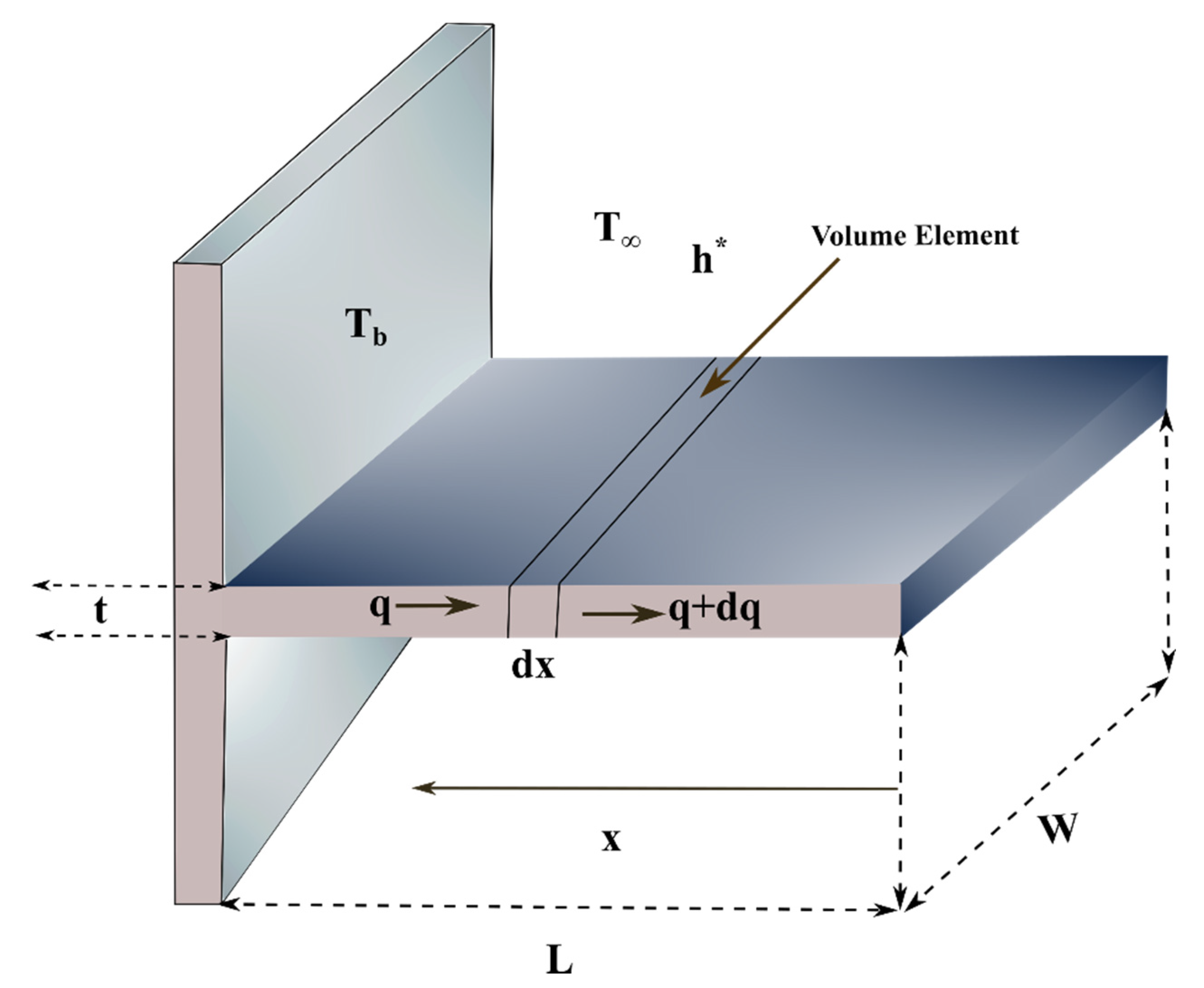
2. Mathematical Formulation

A rectangular straight fin of length $L$, width $W$, thickness $t$ with temperature-dependent internal heat generation $q^{*}\left(T\right)$, thermal conductivity $k^{*}\left(T\right)$ whose faces are subjected to convection heat transfer of coefficient $h^{*}\left(T\right)$ at temperature $T_{\infty }$ is considered in this analysis as shown in Figure 1. Since the cross-section’s temperature distribution is negligible and changes significantly in the longitudinal direction, the nature of the current problem is steady-state heat transfer. The thickness of a longitudinal fin $t$ is comparatively lesser than its width $W$ and length $L$, so it is presumed that the thermal attribute over the fin’s thickness and heat transference from its boundaries is insignificant compared to the heat-dissipation at its adjacent region.

With all these norms, the governing equation for the thermal distribution of a fin is given as (Aziz and Bouaziz [11]):

$$\frac{d}{dx}\left[k^{*}(T)A_{cr}^{*}\frac{dT}{dx}\right]-h^{*}\left(T\right)P\left(T-T_{\infty }\right)+A_{cr}^{*}{q}^{*}(T)=0$$

(1)

The corresponding boundary conditions are specified as:

$$\begin{gathered} x=0 ; \frac{dT}{dx}=0, \\ T=T_b ; x=L. \end{gathered}$$

(2)

The temperature dispersion through a fin is investigated in this study by determining two scenarios:

• $k^{*}\left(T\right)$ and $h^{*}\left(T\right)$ are taken to be exponentially varying with temperature change.
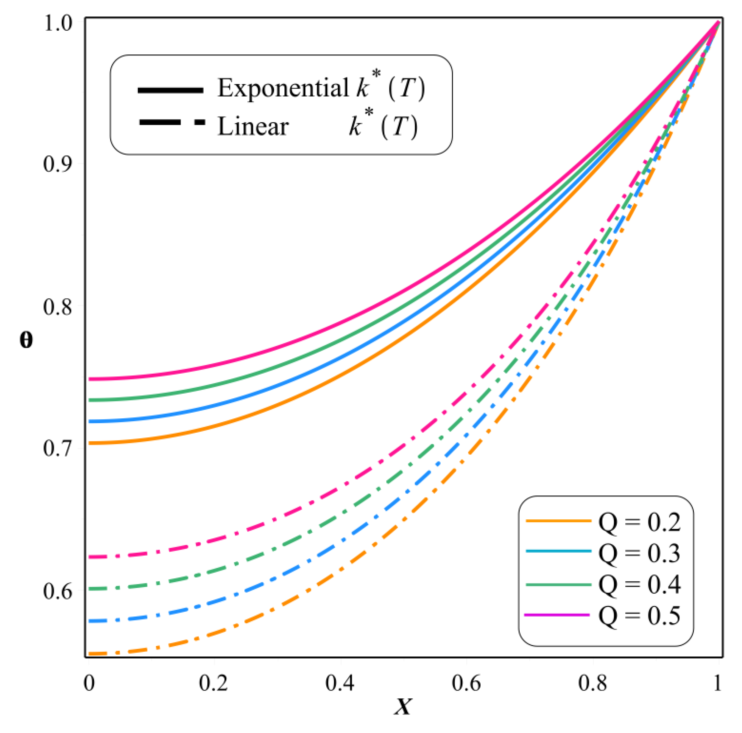
• $k^{*}\left(T\right)$ varies linearly with temperature and $h^{*}\left(T\right)$ exponentially varies with temperature change.

Case 1: Fin with exponential temperature-dependent$k^{*}\left(T\right)$

Here, $k^{*}\left(T\right)$ and $h^{*}\left(T\right)$ depend exponentially on the temperature change and are mathematically expressed as (see Moradi and Ahmadikia [41]):

$$k^{*}(T)=k_0{e}^{a_{0}T} \mathrm{and} h^{*}(T)=h_0{e}^{b_{0}T},$$

(3)

and $q^{*}\left(T\right)$ is signified as:

$$q^{*}(T)=q_a\left[1+\psi \left(T-T_{\infty }\right)\right]$$

(4)

For the sake of ease, the following non-dimensional terms are used.

$$\begin{gathered} \theta =\frac{T-T_{\infty }}{T_b-T_{\infty }}, {\alpha }^2=\frac{P{h}_b{L}^2}{k_a{A}_{cr}^{*}}, \gamma =\psi \left(T_b-T_{\infty }\right), X=\frac{x}{L}, \\ Q=\frac{q_a{A}_{cr}^{*}}{P{h}_b\left(T_b-T_{\infty }\right)}, \beta =\kappa \left(T_b-T_{\infty }\right). \end{gathered}$$

(5)

And Equation (3) is indicated as:

$$k^{*}(T)=k_a{e}^{a\theta } \mathrm{and} h^{*}(T)=h_b{e}^{b\theta }.$$

(6)

where,

$$\begin{gathered} a=a_0\left(T_b-T_{\infty }\right), k_a=k_0{e}^{a_0{T}_{\infty }}, \\ b=b_0\left(T_b-T_{\infty }\right), h_b=h_0{e}^{h_0{T}_{\infty }}. \end{gathered}$$

(7)

Using the above Equation from (3) to (7), Equation (1) together with the boundary conditions (2) can be derived as:

$$\frac{d}{dX}\left[e^{a\theta }\frac{d\theta }{dX}\right]-{\alpha }^2\theta e^{b\theta }+{\alpha }^{2}Q\left(1+\gamma \theta \right)=0,$$

(8)

Subjected to

$$\begin{gathered} \frac{d\theta }{dX}\left(0\right)=0, \\ \theta \left(1\right)=1. \end{gathered}$$

(9)

Case 2: Fin with linear temperature-dependent$k^{*}\left(T\right)$

Here, the thermal conductivity $k^{*}\left(T\right)$ depends linearly on the temperature change, and the $h^{*}\left(T\right)$ depends exponentially on the temperature change and are mathematically expressed as:

$$k^{*}(T)=k_a\left[1+\kappa \left(T-T_{\infty }\right)\right] \mathrm{and} h^{*}(T)=h_0{e}^{b_{0}T}.$$

(10)

And Equation (10) is indicated as:

$$h^{*}(T)=h_b{e}^{b\theta }$$

(11)

where,

$$b=b_0\left(T_b-T_{\infty }\right), h_b=h_0{e}^{h_0{T}_{\infty }}.$$

(12)

Using the above Equation from (10) to (12) with Equation (5), Equation (1) together with the boundary conditions (2) can be derived as:

$$\frac{d^2\theta }{d{X}^2}+\beta \theta \frac{d^2\theta }{d{X}^2}+\beta {\left(\frac{d\theta }{dX}\right)}^2-{\alpha }^2\theta e^{b\theta }+{\alpha }^{2}Q\left(1+\gamma \theta \right)=0$$

(13)

Subjected to

$$\begin{gathered} \frac{d\theta }{dX}\left(0\right)=0, \\ \theta \left(1\right)=1. \end{gathered}$$

(14)

3. The Fundamental Concept of DTM-Pade Approximant

Zhou [31] introduced and applied the idea of DTM to solve linear and non-linear initial value problems in electric circuit investigation. This technique was later implemented to achieve analytical solutions to the partial differential equation (PDE), ODE, and other kinds of equations (see Moradi and Ahmadikia [41], Jawad [42]). Therefore, to derive an analytical solution for the prescribed differential equation, the basic definitions and preliminary results of DTM and Pade approximants are required and are found in the literature Wang et al. [18], Boyd [43], Rashidi et al. [38], and Ismail et al. [44].

4. Solution Procedure with DTM-Pade Approximant

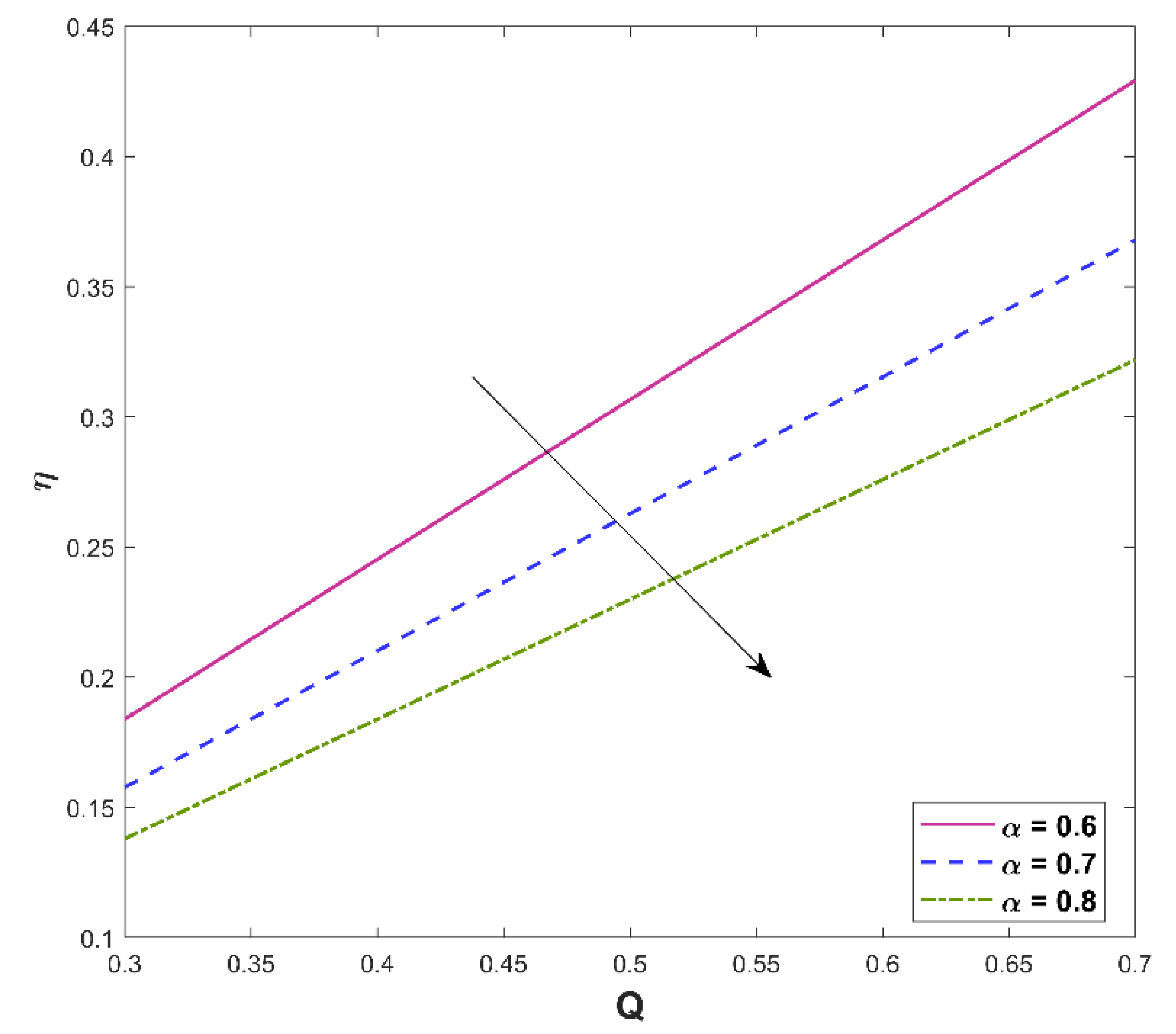
Case 1: Fin with Exponential$k^{*}\left(T\right)$

Equation (8) is transformed using the DTM technique as:

$$\begin{array}{l}{\displaystyle \sum _{s=0}^{{\rm K}}}F\left[s\right]\left({\rm K}-s+1\right)\left({\rm K}-s+2\right) \mathsf{\Theta }\left[{\rm K}-s+2\right]+a{\displaystyle \sum _{s=0}^{{\rm K}}} \left(s+1\right) \mathsf{\Theta }\left[s+1\right] {\displaystyle \sum _{l=0}^{{\rm K}-s}} F\left[l\right]\left({\rm K}-s-l+1\right)\mathsf{\Theta }\left[{\rm K}-s-l+1\right]-\\ \\ {\alpha }^2{\displaystyle \sum _{s=0}^{{\rm K}}}G\left[s\right]\mathsf{\Theta }\left[{\rm K}-s\right]+{\alpha }^{2}Q\left(\Delta \left[{\rm K}\right]+\gamma \mathsf{\Theta }\left[{\rm K}\right]\right)=0\end{array}$$

(15)

The transformed function $F [s]$, $F [l]$ and $G [s]$ of $e^{a\theta }$ and $e^{b\theta }$ in the Equation (15) are evaluated using the basic properties of DTM (see Moradi and Ahmadikia [41]) and $\mathsf{\Theta }\left[{\rm K}\right]$ is the differential transform of $\theta \left(X\right)$.

After applying DTM to Equation (9), the transformed relation is given as;

$$\begin{gathered} \mathsf{\Theta }\left[0\right]=A, \mathsf{\Theta }\left[1\right]=0, \\ {\displaystyle \sum _{r=0}^{\infty }}\mathsf{\Theta }\left[r\right]=1 \end{gathered}$$

(16)

Substituting Equation (16) and ${\rm K}=0, 1, 2, 3\dots$ in Equation (15), The consecutive approximants are derived as follows:

$$\begin{gathered} \mathsf{\Theta }\left[2\right]=\frac{1}{2{\mathrm{e}}^{aA}} {\alpha }^2\left(-A\gamma Q+A{\mathrm{e}}^{bA}-Q\right) \\ \mathsf{\Theta }\left[3\right]=0 \end{gathered}$$

(17)

$$\mathsf{\Theta }\left[4\right]=-\frac{1}{24{\left({\mathrm{e}}^{aA}\right)}^2} {\alpha }^4\left(\begin{array}{l}3A^2{\gamma }^2{Q}^{2}a-6A^2\gamma {\mathrm{e}}^{bA}Qa+A^2\gamma {\mathrm{e}}^{bA}Qb+3A^2{\left({\mathrm{e}}^{bA}\right)}^{2}a-A^2{\left({\mathrm{e}}^{bA}\right)}^{2}b-A{\gamma }^2{Q}^2+\\ 6A\gamma Q^{2}a+2A\gamma {\mathrm{e}}^{bA}Q-6A{\mathrm{e}}^{bA}Qa+A{\mathrm{e}}^{bA}Qb-A{\left({\mathrm{e}}^{bA}\right)}^2-\gamma Q^2+3Q^{2}a+{\mathrm{e}}^{bA}Q\end{array}\right)$$

(18)

$$\mathsf{\Theta }\left[5\right]=0$$

(19)

$$\mathsf{\Theta }\left[6\right]=-\frac{1}{720{\left({\mathrm{e}}^{aA}\right)}^3} {\alpha }^6 \left(\begin{array}{l}-90A^3{\gamma }^2{\mathrm{e}}^{bA}{Q}^2{a}^2-3A^3{\gamma }^2{\mathrm{e}}^{bA}{Q}^2{b}^2+90A^3\gamma {\left({\mathrm{e}}^{bA}\right)}^{2}Q{a}^2+7A^3\gamma {\left({\mathrm{e}}^{bA}\right)}^{2}Q{b}^2+54A^2{\gamma }^2{\mathrm{e}}^{bA}{Q}^{2}a-\\ \\ 8A^2{\gamma }^2{\mathrm{e}}^{bA}{Q}^{2}b-180A^2\gamma {\mathrm{e}}^{bA}{Q}^2{a}^2-6A^2\gamma {\mathrm{e}}^{bA}{Q}^2{b}^2-54A^2\gamma {\left({\mathrm{e}}^{bA}\right)}^{2}Qa+16A^2\gamma {\left({\mathrm{e}}^{bA}\right)}^{2}Qb-\\ \\ 36A^2{\left({\mathrm{e}}^{bA}\right)}^{2}Qab+72A\gamma {\mathrm{e}}^{bA}{Q}^{2}a-14A\gamma {\mathrm{e}}^{bA}{Q}^{2}b+18A{\mathrm{e}}^{bA}{Q}^{2}ab+90A\gamma Q^3{a}^2-3A{\gamma }^2{\mathrm{e}}^{bA}{Q}^2-\\ \\ 90A{\mathrm{e}}^{bA}{Q}^2{a}^2-3A{\mathrm{e}}^{bA}{Q}^2{b}^2+3A\gamma {\left({\mathrm{e}}^{bA}\right)}^{2}Q-36A{\left({\mathrm{e}}^{bA}\right)}^{2}Qa+14A{\left({\mathrm{e}}^{bA}\right)}^{2}Qb+18A^3{\gamma }^2{\mathrm{e}}^{bA}{Q}^{2}ab-\\ \\ 36A^3\gamma {\left({\mathrm{e}}^{bA}\right)}^{2}Qab+36A^2\gamma {\mathrm{e}}^{bA}{Q}^{2}ab+30Q^3{a}^2+{\gamma }^2{Q}^3-A{\left({\mathrm{e}}^{bA}\right)}^3+{\left({\mathrm{e}}^{bA}\right)}^{2}Q-30A^3{\left({\mathrm{e}}^{bA}\right)}^3{a}^2-\\ \\ 4A^3{\left({\mathrm{e}}^{bA}\right)}^3{b}^2+A{\gamma }^3{Q}^3+18A^2{\left({\mathrm{e}}^{bA}\right)}^{3}a-8A^2{\left({\mathrm{e}}^{bA}\right)}^{3}b-18\gamma Q^{3}a-2\gamma {\mathrm{e}}^{bA}{Q}^2+18{\mathrm{e}}^{bA}{Q}^{2}a-\\ \\ 6{\mathrm{e}}^{bA}{Q}^{2}b+30A^3{\gamma }^3{Q}^3{a}^2-18A^2{\gamma }^3{Q}^{3}a+90A^2{\gamma }^2{Q}^3{a}^2+18A^3{\left({\mathrm{e}}^{bA}\right)}^{3}ab+90A^2{\left({\mathrm{e}}^{bA}\right)}^{2}Q{a}^2+\\ \\ 7A^2{\left({\mathrm{e}}^{bA}\right)}^{2}Q{b}^2-36A{\gamma }^2{Q}^{3}a\end{array}\right)$$

(20)

And so on.

Where the constant $A$, which has to be evaluated by employing Equation (9). We have developed a power series of order 6 utilizing Equations (16)–(20), which is expressed as:

$$\begin{gathered} \theta \left(X\right) = A+ \frac{1}{2{\mathrm{e}}^{aA}} {\alpha }^2\left(-A\gamma Q+A{\mathrm{e}}^{bA}-Q\right)X^2-\frac{1}{24{\left({\mathrm{e}}^{aA}\right)}^2} {\alpha }^4\left(\begin{array}{l}3A^2{\gamma }^2{Q}^{2}a-6A^2\gamma {\mathrm{e}}^{bA}Qa+A^2\gamma {\mathrm{e}}^{bA}Qb+3A^2{\left({\mathrm{e}}^{bA}\right)}^{2}a-A^2{\left({\mathrm{e}}^{bA}\right)}^{2}b-A{\gamma }^2{Q}^2+\\ \\ 6A\gamma Q^{2}a+2A\gamma {\mathrm{e}}^{bA}Q-6A{\mathrm{e}}^{bA}Qa+A{\mathrm{e}}^{bA}Qb-A{\left({\mathrm{e}}^{bA}\right)}^2-\gamma Q^2+3Q^{2}a+{\mathrm{e}}^{bA}Q\end{array}\right)X^4- \\ \frac{1}{720{\left({\mathrm{e}}^{aA}\right)}^3} {\alpha }^6 \left(\begin{array}{l}-90A^3{\gamma }^2{\mathrm{e}}^{bA}{Q}^2{a}^2-3A^3{\gamma }^2{\mathrm{e}}^{bA}{Q}^2{b}^2+90A^3\gamma {\left({\mathrm{e}}^{bA}\right)}^{2}Q{a}^2+7A^3\gamma {\left({\mathrm{e}}^{bA}\right)}^{2}Q{b}^2+54A^2{\gamma }^2{\mathrm{e}}^{bA}{Q}^{2}a-8A^2{\gamma }^2{\mathrm{e}}^{bA}{Q}^{2}b-180A^2\gamma {\mathrm{e}}^{bA}{Q}^2{a}^2-6A^2\gamma {\mathrm{e}}^{bA}{Q}^2{b}^2-\\ \\ 54A^2\gamma {\left({\mathrm{e}}^{bA}\right)}^{2}Qa+16A^2\gamma {\left({\mathrm{e}}^{bA}\right)}^{2}Qb-36A^2{\left({\mathrm{e}}^{bA}\right)}^{2}Qab+72A\gamma {\mathrm{e}}^{bA}{Q}^{2}a-14A\gamma {\mathrm{e}}^{bA}{Q}^{2}b+18A{\mathrm{e}}^{bA}{Q}^{2}ab+90A\gamma Q^3{a}^2-3A{\gamma }^2{\mathrm{e}}^{bA}{Q}^2-90A{\mathrm{e}}^{bA}{Q}^2{a}^2-\\ \\ 3A{\mathrm{e}}^{bA}{Q}^2{b}^2+3A\gamma {\left({\mathrm{e}}^{bA}\right)}^{2}Q-36A{\left({\mathrm{e}}^{bA}\right)}^{2}Qa+14A{\left({\mathrm{e}}^{bA}\right)}^{2}Qb+18A^3{\gamma }^2{\mathrm{e}}^{bA}{Q}^{2}ab-36A^3\gamma {\left({\mathrm{e}}^{bA}\right)}^{2}Qab+36A^2\gamma {\mathrm{e}}^{bA}{Q}^{2}ab+30Q^3{a}^2+{\gamma }^2{Q}^3-A{\left({\mathrm{e}}^{bA}\right)}^3\\ \\ +{\left({\mathrm{e}}^{bA}\right)}^{2}Q-30A^3{\left({\mathrm{e}}^{bA}\right)}^3{a}^2-4A^3{\left({\mathrm{e}}^{bA}\right)}^3{b}^2+A{\gamma }^3{Q}^3+18A^2{\left({\mathrm{e}}^{bA}\right)}^{3}a-8A^2{\left({\mathrm{e}}^{bA}\right)}^{3}b-18\gamma Q^{3}a-2\gamma {\mathrm{e}}^{bA}{Q}^2+18{\mathrm{e}}^{bA}{Q}^{2}a-6{\mathrm{e}}^{bA}{Q}^{2}b+\\ \\ 30A^3{\gamma }^3{Q}^3{a}^2-18A^2{\gamma }^3{Q}^{3}a+90A^2{\gamma }^2{Q}^3{a}^2+18A^3{\left({\mathrm{e}}^{bA}\right)}^{3}ab+90A^2{\left({\mathrm{e}}^{bA}\right)}^{2}Q{a}^2+7A^2{\left({\mathrm{e}}^{bA}\right)}^{2}Q{b}^2-36A{\gamma }^2{Q}^{3}a\end{array}\right)X^6 \end{gathered}$$

(21)

The $A$ value is extracted by applying the Pade approximant to Equation (21) with Equation (9). The constant value $A=0.9954320629,$ $Q=0.2,$$a=1,$$\alpha =0.1,$$b=1,$ $\gamma =0.1$ are substituted in the series, we get

$$\begin{array}{l}\theta \left(X\right)=0.9954320629+0.004570809020X^2-0.000002873685247X^4+\\ 5.745191892\times {10}^{-9}{X}^6+\dots \end{array}$$

(22)

Case 2: Fin with Linear$k^{*}\left(T\right)$

Equation (13) is transformed using the DTM technique as:

$$\begin{array}{l}\left({\rm K}+1\right)\left({\rm K}+2\right)\mathsf{\Theta }\left[{\rm K}+2\right]+\beta {\displaystyle \underset{s=0}{\overset{{\rm K}}{ \sum }}}\left(s+1\right)\mathsf{\Theta }\left[s+1\right] \left({\rm K}-s+1\right)\mathsf{\Theta }\left[{\rm K}-s+1\right]+\beta {\displaystyle \sum _{s=0}^{{\rm K}}} \mathsf{\Theta }\left[{\rm K}-s\right]\left(s+1\right)\left(s+2\right)\mathsf{\Theta }\left[s+2\right]-\\ \\ {\alpha }^2{\displaystyle \underset{s=0}{\overset{{\rm K}}{ \sum }}} G\left[s\right]\mathsf{\Theta }\left[{\rm K}-s\right]+{\alpha }^2 Q \left(\gamma \mathsf{\Theta }\left[{\rm K}\right]+\Delta \left[{\rm K}\right]\right)=0\end{array}$$

(23)

applying DTM to Equation (14) yields

$$\begin{gathered} \mathsf{\Theta }\left[0\right]=B, \mathsf{\Theta }\left[1\right]=0, \\ {\displaystyle \sum _{r=0}^{\infty }}\mathsf{\Theta }\left[r\right]=1 \end{gathered}$$

(24)

Substituting Equation (24) and ${\rm K}=0, 1, 2, 3\dots$ in Equation (23), The consecutive approximants are derived as follows:

$$\mathsf{\Theta }\left[2\right]=\frac{1}{2\left(B\beta +1\right)}{\alpha }^2\left(-B\gamma Q+B{\mathrm{e}}^{bB}-Q\right)$$

(25)

$$\mathsf{\Theta }\left[3\right]=0$$

(26)

$$\mathsf{\Theta }\left[4\right]=\frac{1}{24{\left(B\beta +1\right)}^3}\left[{\alpha }^4\left(-B\gamma Q+B{\mathrm{e}}^{bB}-Q\right)\left(B^2{\mathrm{e}}^{bB}b\beta +2B\gamma Q\beta +B{\mathrm{e}}^{bB}b-2B{\mathrm{e}}^{bB}\beta -Q\gamma +3Q\beta +{\mathrm{e}}^{bB}\right)\right]$$

(27)

$$\mathsf{\Theta }\left[5\right]=0$$

(28)

$$\mathsf{\Theta }\left[6\right]=\frac{1}{720{\left(B\beta +1\right)}^5} \left\{{\alpha }^6\left(B\gamma Q-B{\mathrm{e}}^{bB}+Q\right)\left(\begin{array}{l}-{\left({\mathrm{e}}^{bB}\right)}^2+3B^3{\mathrm{e}}^{bB}Q{b}^2{\beta }^2+3B^2\gamma {\mathrm{e}}^{bB}Q{b}^2+56B^2\gamma {\mathrm{e}}^{bB}Q{\beta }^2+6B^2{\mathrm{e}}^{bB}Q{b}^2\beta -\\ \\ 12B^2{\mathrm{e}}^{bB}Qb{\beta }^2+8B\gamma {\mathrm{e}}^{bB}Qb-32B\gamma {\mathrm{e}}^{bB}Q\beta -6B{\mathrm{e}}^{bB}Qb\beta -4B^4{\left({\mathrm{e}}^{bB}\right)}^2{b}^2{\beta }^2-\\ \\ 8B^3{\left({\mathrm{e}}^{bB}\right)}^2{b}^2\beta +10B^3{\left({\mathrm{e}}^{bB}\right)}^{2}b{\beta }^2-28B^2{\gamma }^2{Q}^2{\beta }^2+2B^2{\left({\mathrm{e}}^{bB}\right)}^{2}b\beta +16B{\gamma }^2{Q}^2\beta -\\ \\ 72B\gamma Q^2{\beta }^2+3B{\mathrm{e}}^{bB}Q{b}^2+72B{\mathrm{e}}^{bB}Q{\beta }^2+3B^4\gamma {\mathrm{e}}^{bB}Q{b}^2{\beta }^2+6B^3\gamma {\mathrm{e}}^{bB}Q{b}^2\beta -\\ \\ 10B^3\gamma {\mathrm{e}}^{bB}Qb{\beta }^2-2B^2\gamma {\mathrm{e}}^{bB}Qb\beta -4B^2{\left({\mathrm{e}}^{bB}\right)}^2{b}^2-28B^2{\left({\mathrm{e}}^{bB}\right)}^2{\beta }^2-8B{\left({\mathrm{e}}^{bB}\right)}^{2}b+\\ \\ 16B{\left({\mathrm{e}}^{bB}\right)}^2\beta +18\gamma Q^2\beta +2\gamma {\mathrm{e}}^{bB}Q+6{\mathrm{e}}^{bB}Qb-18{\mathrm{e}}^{bB}Q\beta -45Q^2{\beta }^2-{\gamma }^2{Q}^2\end{array}\right)\right\}$$

(29)

And so on.

Where the constant $B$, which has to be evaluated by employing Equation (14). We have developed a power series of order 6 utilizing Equations (24)–(29), which is expressed as:

$$\begin{array}{l}\theta \left(X\right) = A+\frac{1}{2\left(B\beta +1\right)}{\alpha }^2\left(-B\gamma Q+B{\mathrm{e}}^{bB}-Q\right) X^2+\frac{1}{24{\left(B\beta +1\right)}^3}\left[{\alpha }^4\left(-B\gamma Q+B{\mathrm{e}}^{bB}-Q\right)\left(\begin{array}{l}{B}^2{\mathrm{e}}^{bB}b\beta +2B\gamma Q\beta +B{\mathrm{e}}^{bB}b-2B{\mathrm{e}}^{bB}\beta \\ -Q\gamma +3Q\beta +{\mathrm{e}}^{bB}\end{array}\right)\right]X^4+\\ \\ \frac{1}{720{\left(B\beta +1\right)}^5} \left\{{\alpha }^6\left(B\gamma Q-B{\mathrm{e}}^{bB}+Q\right)\left(\begin{array}{l}-{\left({\mathrm{e}}^{bB}\right)}^2+3B^3{\mathrm{e}}^{bB}Q{b}^2{\beta }^2+3B^2\gamma {\mathrm{e}}^{bB}Q{b}^2+56B^2\gamma {\mathrm{e}}^{bB}Q{\beta }^2+6B^2{\mathrm{e}}^{bB}Q{b}^2\beta -\\ 12B^2{\mathrm{e}}^{bB}Qb{\beta }^2+8B\gamma {\mathrm{e}}^{bB}Qb-32B\gamma {\mathrm{e}}^{bB}Q\beta -6B{\mathrm{e}}^{bB}Qb\beta -4B^4{\left({\mathrm{e}}^{bB}\right)}^2{b}^2{\beta }^2-\\ 8B^3{\left({\mathrm{e}}^{bB}\right)}^2{b}^2\beta +10B^3{\left({\mathrm{e}}^{bB}\right)}^{2}b{\beta }^2-28B^2{\gamma }^2{Q}^2{\beta }^2+2B^2{\left({\mathrm{e}}^{bB}\right)}^{2}b\beta +16B{\gamma }^2{Q}^2\beta -\\ 72B\gamma Q^2{\beta }^2+3B{\mathrm{e}}^{bB}Q{b}^2+72B{\mathrm{e}}^{bB}Q{\beta }^2+3B^4\gamma {\mathrm{e}}^{bB}Q{b}^2{\beta }^2+6B^3\gamma {\mathrm{e}}^{bB}Q{b}^2\beta -\\ 10B^3\gamma {\mathrm{e}}^{bB}Qb{\beta }^2-2B^2\gamma {\mathrm{e}}^{bB}Qb\beta -4B^2{\left({\mathrm{e}}^{bB}\right)}^2{b}^2-28B^2{\left({\mathrm{e}}^{bB}\right)}^2{\beta }^2-8B{\left({\mathrm{e}}^{bB}\right)}^{2}b+\\ 16B{\left({\mathrm{e}}^{bB}\right)}^2\beta +18\gamma Q^2\beta +2\gamma {\mathrm{e}}^{bB}Q+6{\mathrm{e}}^{bB}Qb-18{\mathrm{e}}^{bB}Q\beta -45Q^2{\beta }^2-{\gamma }^2{Q}^2\end{array}\right)\right\}{X}^6+\dots \end{array}$$

(30)

The $B$ value is extracted by applying the Pade approximant to Equation (30) with Equation (14). The constant value $B=0.9888654429,$ $Q=0.2,$$\beta =0.1,$$\alpha =0.1,$$b=1,$ $\gamma =0.1$ are substituted in the series, we get

$$\begin{array}{l}\theta \left(X\right)=0.9888654429+0.01109520280X^2+0.00003921518999X^4+\\ {1.73779481310}^{-7}{X}^6+\dots \end{array}$$

(31)

5. Fin Efficiency

Fin efficiency is stated as the ratio of the fin heat transference rate to the rate that it would be if the complete fin were maintained at the base temperature and is mathematically expressed as:

$$\eta =\frac{k^{*}{A}_{cr}^{*}{\frac{dT}{dx}}_{x=L}}{P{h}^{*}L\left(T_b-T_{\infty }\right)}$$

(32)

The dimensionless form of fin efficiency is expressed as:

$$\eta =\frac{e^{a-b}{\theta }^{\prime }\left(1\right)}{{\alpha }^2}$$

(33)

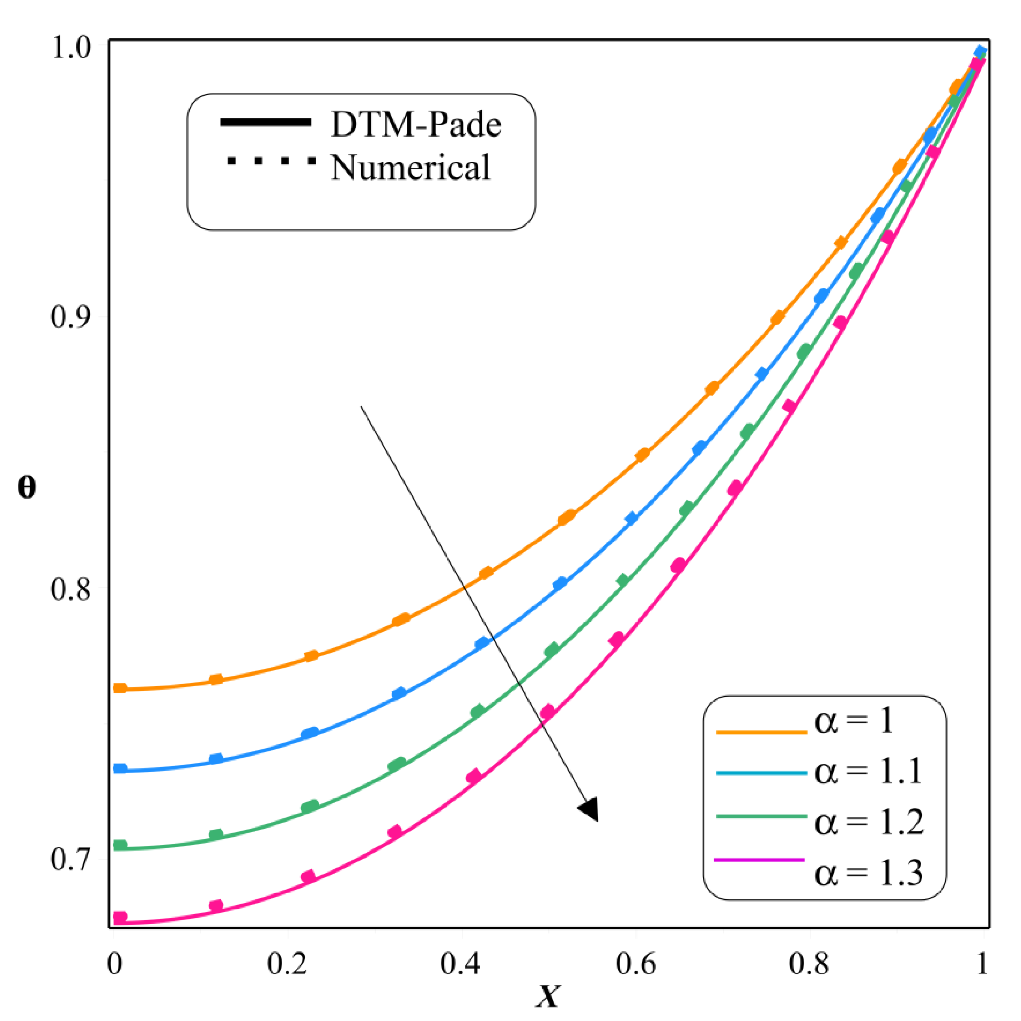
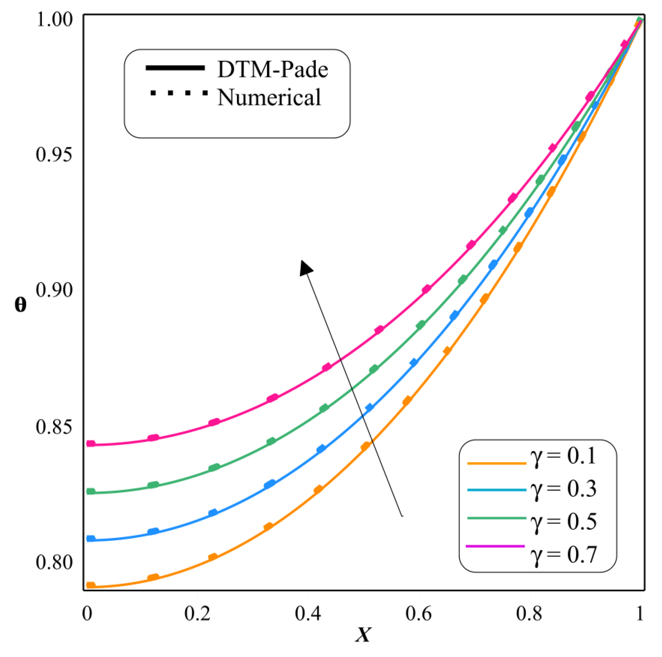
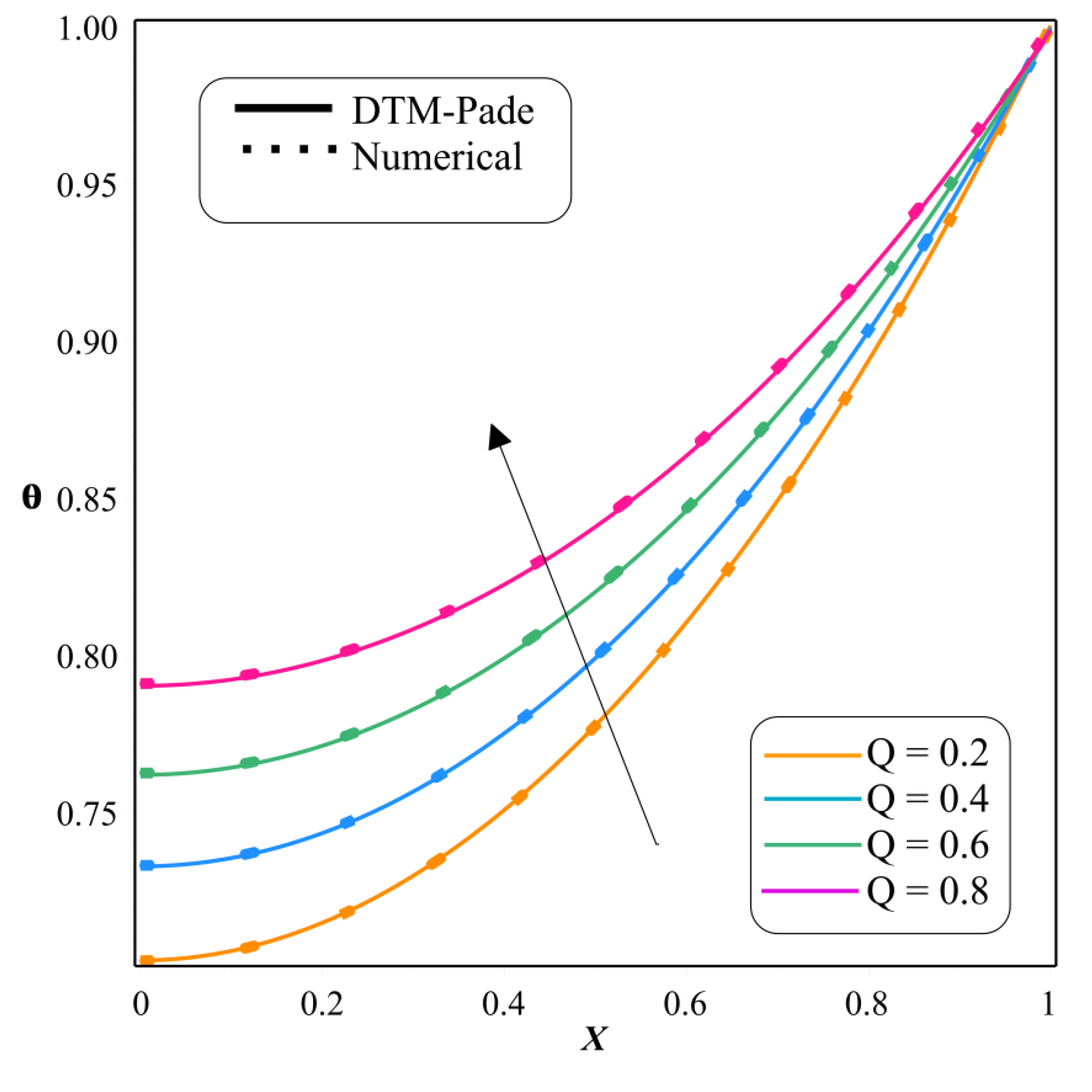
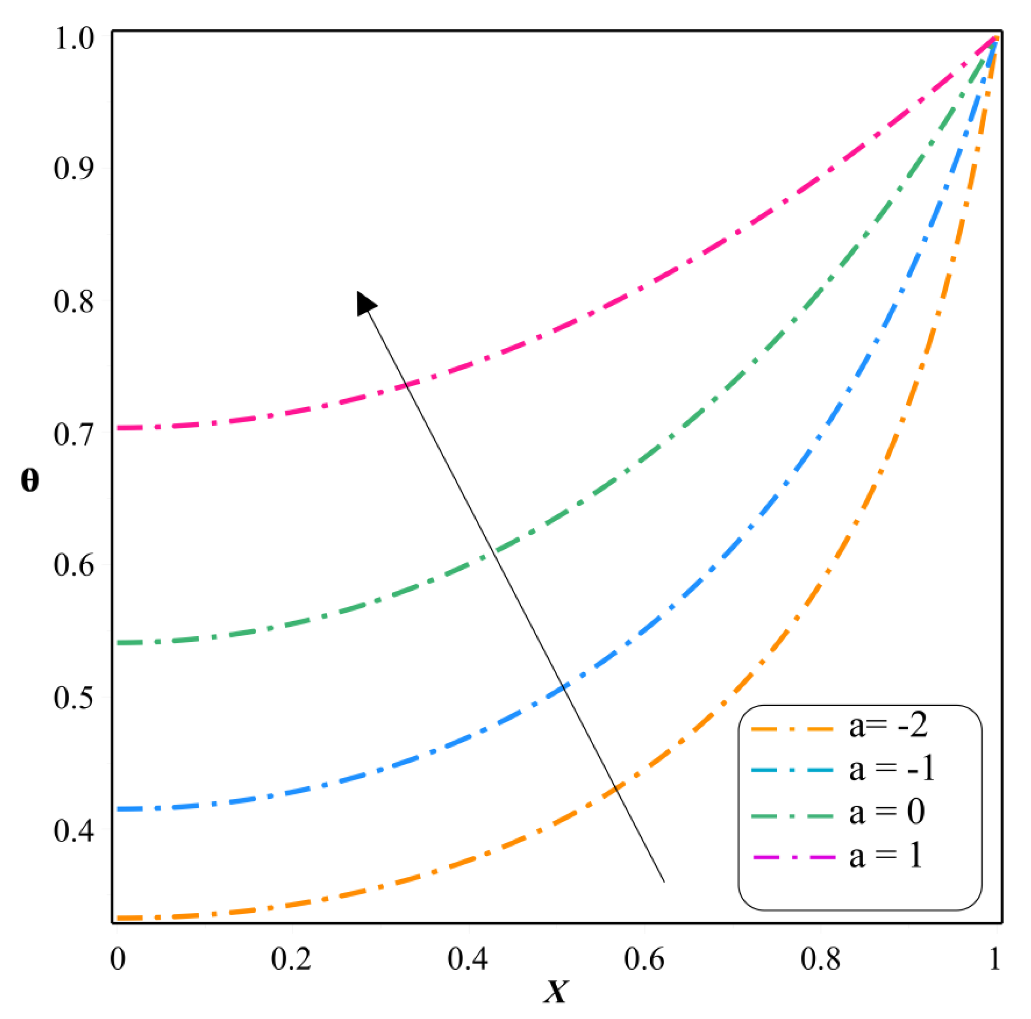
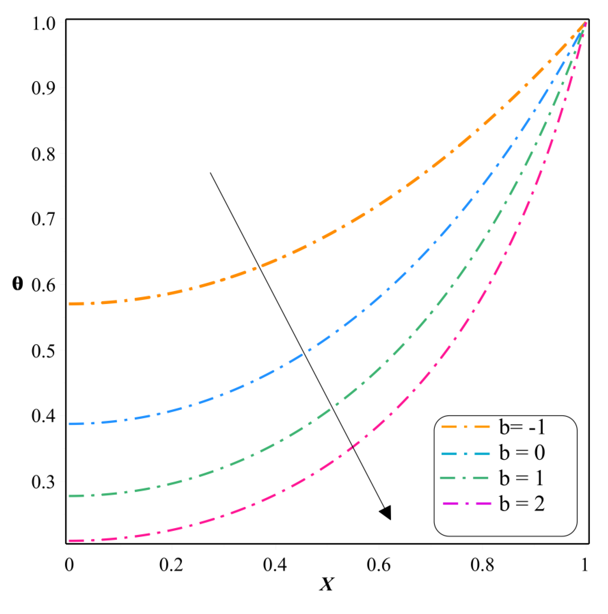
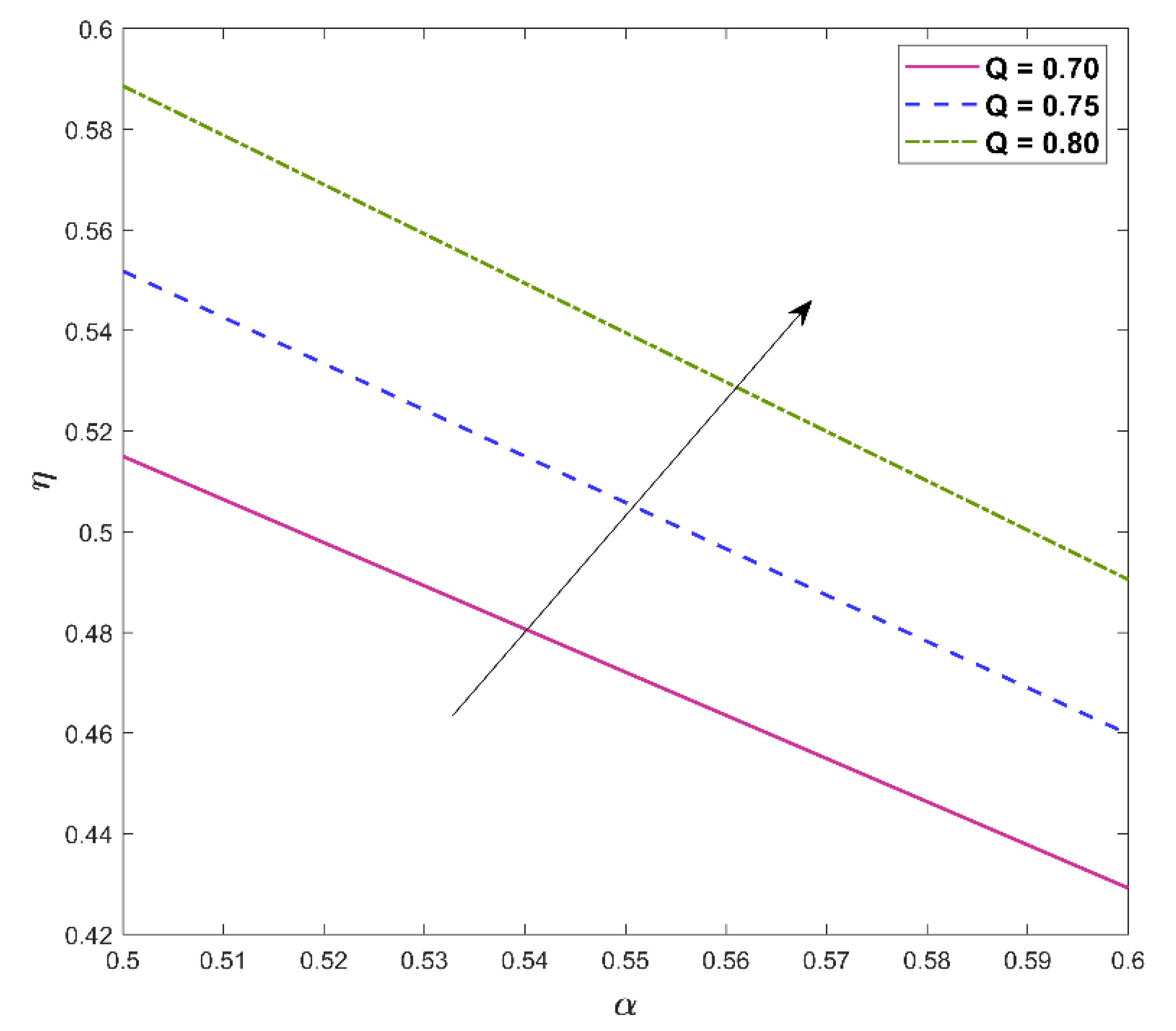
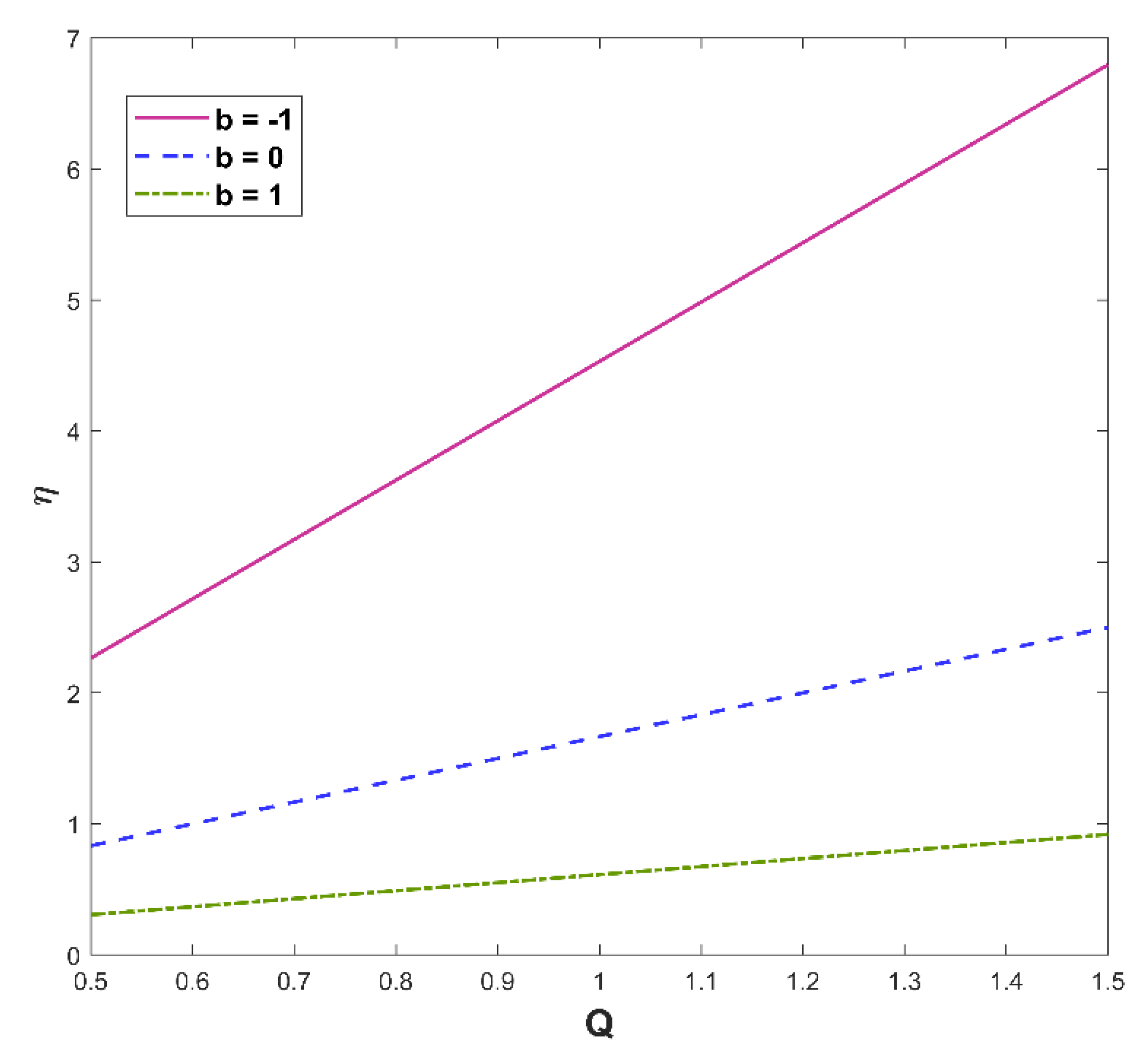
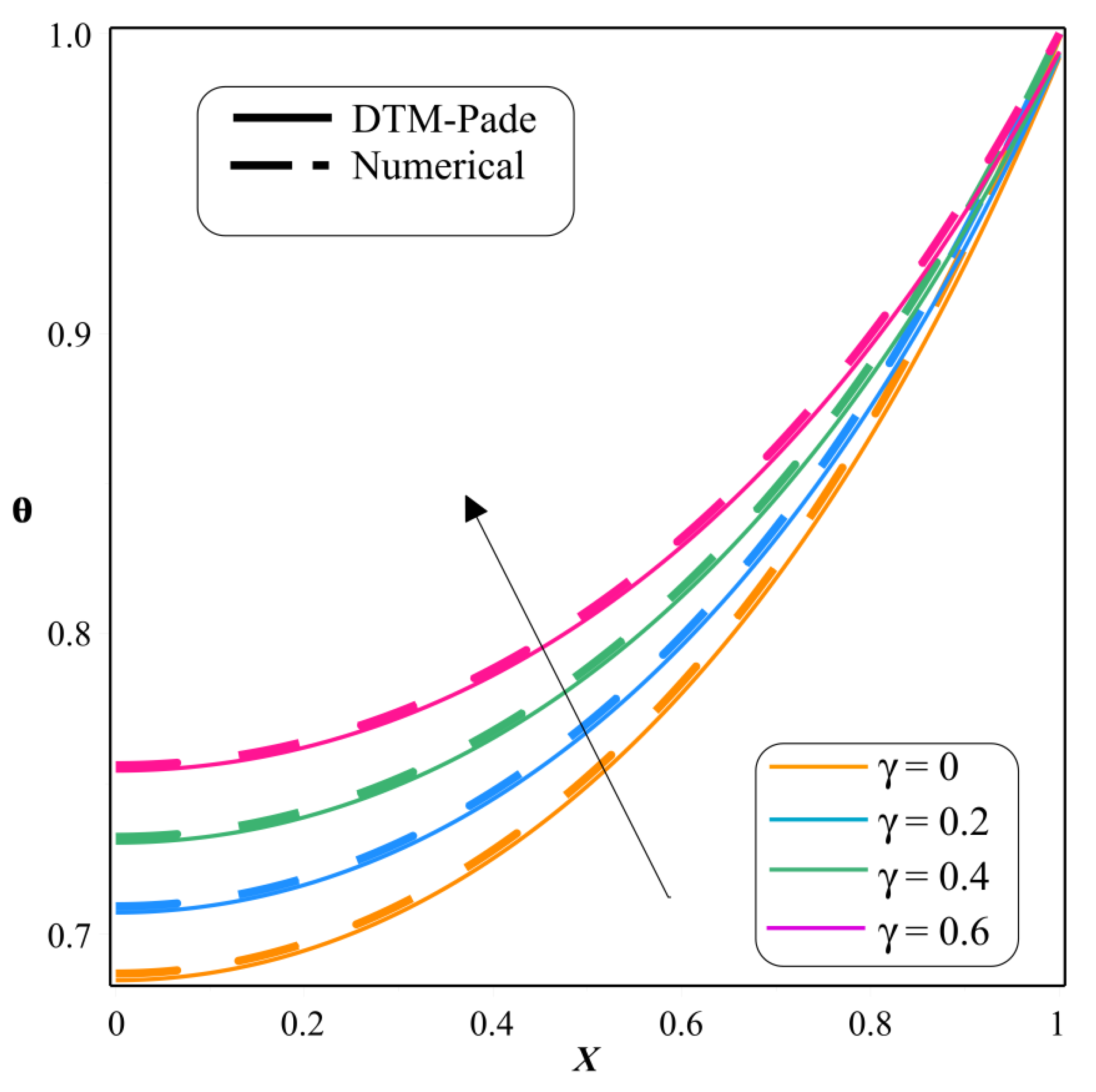
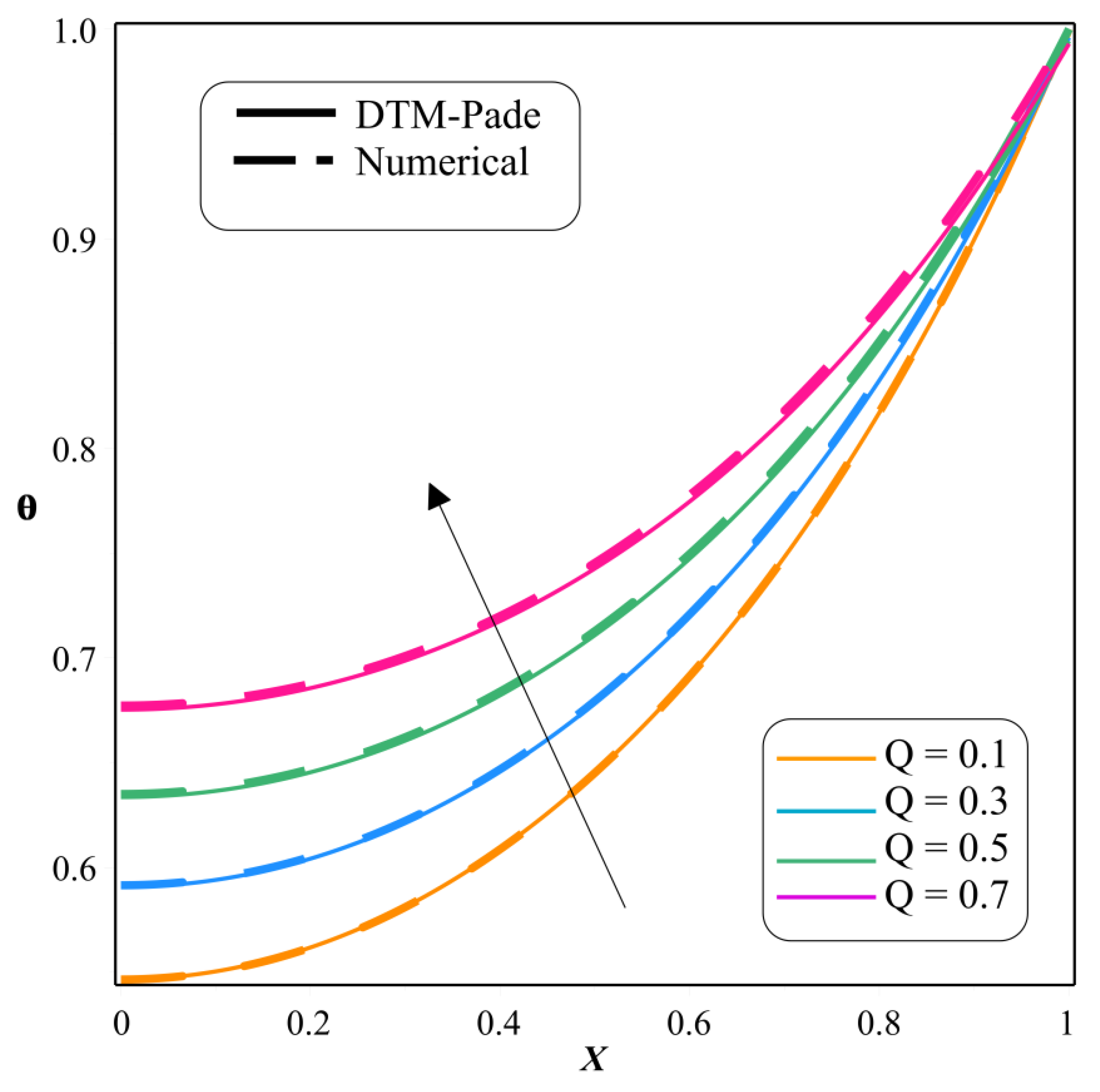
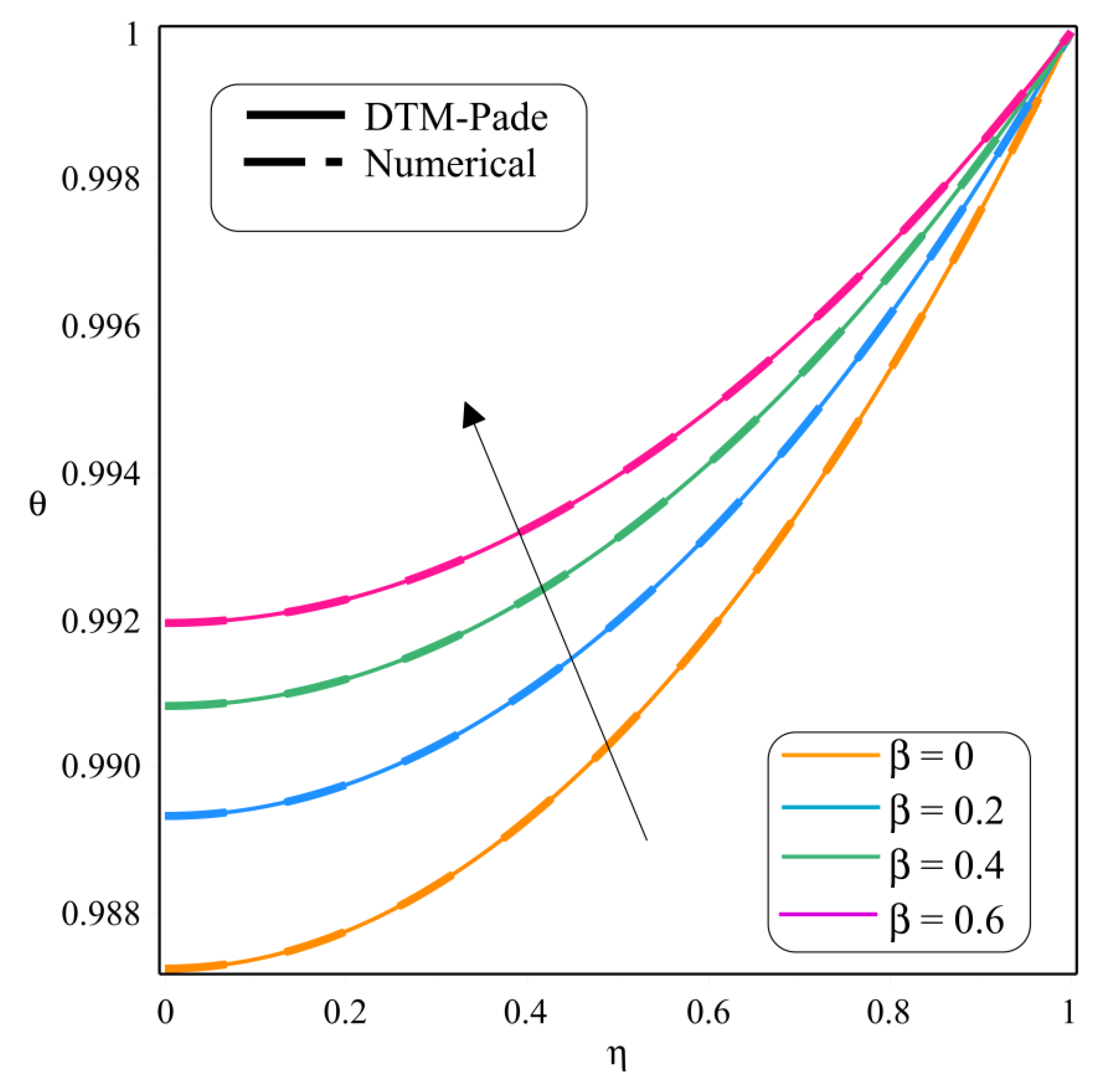
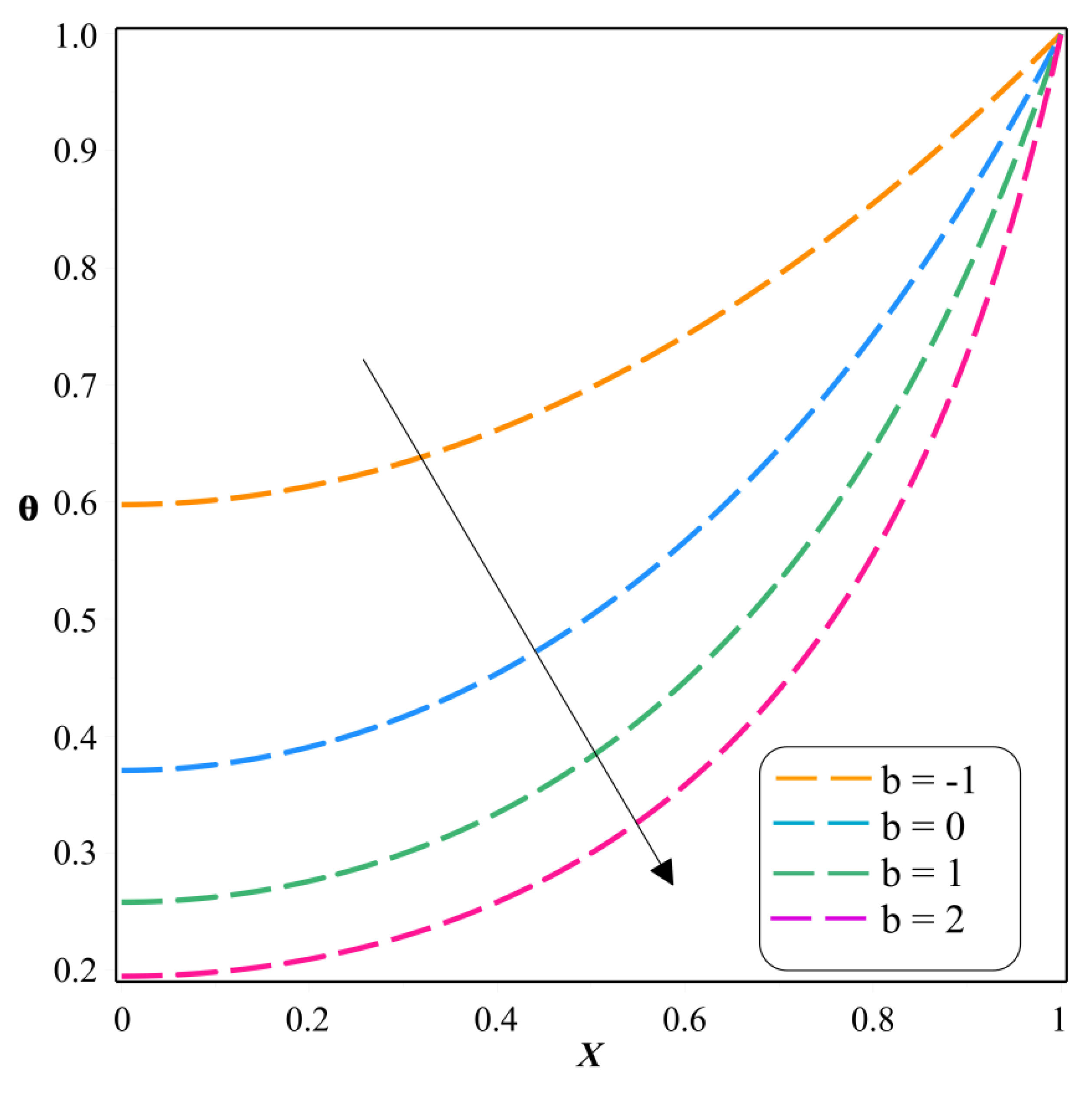
6. Result and Discussion

The significant consequence of several dimensionless variables, namely thermal conductivity parameter $\beta ,$ thermo-geometric parameter $\alpha$, internal heat generation variable $\gamma$, and heat transfer parameter $Q$ on the thermal dispersal of a longitudinal rectangular fin with exponential temperature-dependent heat transfer coefficient is examined by considering two cases of thermal conductivity. In the first case, it is taken to be exponential temperature-dependent, whereas in the other case, it is linearly dependent on temperature. The significance of these pertinent parameters on the non-dimensional temperature profile $\theta$ is explained in this section via graphical representation for both the aforementioned cases by using the DTM-Pade and RKF-45 methods.

Also, the effect of parameters on fin efficiency $\eta$ is debriefed graphically.

Table 1. Comparison of $\theta \left(X\right)$ obtained by DTM-Pade with existing literature (Languri et al. [45]) with constant values of $\beta =0$, $Q=0, \alpha =0.5, b=0, \gamma =0$.

$\mathit{\theta }\left(\mathit{X}\right)$
$\mathbf{X}$	HPM (Languri et al. [45])	VIM (Languri et al. [45])	DTM-Pade	Error
0	0.886819	0.886819	0.886818	0.000001
0.2	0.891257	0.891257	0.891256	0.000001
0.4	0.904614	0.904614	0.904614	0.000000
0.6	0.927026	0.927026	0.927026	0.000000
0.8	0.958715	0.958715	0.958715	0.000000
1.0	1.000000	1.000000	1.000000	0.000000

is developed to compare the results of the current DTM-Pade solution for temperature profile with the existing literature (Languri et al. [45]) to authenticate the correctness of the solution. As per the tabulated result, there is an appropriate consistency between the result of the present work and those in Languri et al. [45], signifying that the solution obtained by the proposed technique is accurate.

Table 2. Comparison of $\theta \left(X\right)$ for $a=-1$, $a=0$ and $a=1$ with constant values of $Q=0.8, \alpha =1, b=1, \gamma =0.5$ obtained by RKF-45 and DTM-Pade.

$\mathit{\theta }\left(\mathit{X}\right)$
$\mathbf{X}$	$\mathit{a}=-1$			$\mathit{a}=0$			$\mathit{a}=1$
	RKF-45	Present Result	$\%\mathbf{Error}$	RKF-45	Present Result	$\%\mathbf{Error}$	RKF-45	Present Result	$\%\mathbf{Error}$
0	0.651268	0.647021	0.4247	0.726859	0.724623	0.2236	0.825904	0.825302	0.0602
0.1	0.653087	0.648719	0.4368	0.728928	0.726658	0.2270	0.827560	0.826954	0.0606
0.2	0.658660	0.653921	0.4739	0.735203	0.732824	0.2379	0.832539	0.831920	0.0619
0.3	0.668357	0.662962	0.5395	0.745885	0.743321	0.2564	0.840872	0.840234	0.0638
0.4	0.682846	0.676443	0.6403	0.761322	0.758489	0.2833	0.852614	0.851948	0.0666
0.5	0.703190	0.695290	0.7900	0.782032	0.778828	0.3204	0.867838	0.867136	0.0702

and

Table 3. Comparison of $\theta \left(X\right)$ for $b=-1$, $b=0$ and $b=1$ with constant values of $Q=0.8, \alpha =1, \gamma =0.5, \beta =0.1$ obtained by RKF-45 and DTM-Pade.

$\mathit{\theta }\left(\mathit{X}\right)$
$\mathbf{X}$	$\mathit{b}=-1$			$\mathit{b}=0$			$\mathit{b}=1$
	RKF-45	Present Result	$\%\mathbf{Error}$	RKF-45	Present Result	$\%\mathbf{Error}$	RKF-45	PresentResult	$\%\mathbf{Error}$
0	1.445973	1.445763	0.0210	1.073794	1.073862	0.0068	0.735737	0.733681	0.2056
0.1	1.441440	1.441231	0.0209	1.073090	1.073158	0.0068	0.737796	0.735710	0.2086
0.2	1.427851	1.427642	0.0209	1.070976	1.071045	0.0069	0.744036	0.741857	0.2179
0.3	1.405233	1.405026	0.0207	1.067438	1.067508	0.0070	0.754636	0.752300	0.2336
0.4	1.373631	1.373427	0.0204	1.062457	1.062528	0.0071	0.769912	0.767346	0.2566
0.5	1.333109	1.332909	0.0200	1.056002	1.056075	0.0073	0.790323	0.787444	0.2879

are constructed to endorse the results achieved from the DTM-Pade and RKF-45 schemes for exponential temperature-dependent and linearly temperature-dependent thermal conductivity, respectively, and are close to each other. The present work is validated graphically with the existing work (Sun and Li [46]) as exhibited in Figure 2 by considering the values of the parameters $a=-1$, $b= 0$, $\alpha = 1.6$, $Q = \gamma =0$ and the graph shows the excellent agreement with the existing work.

Figure 3 illustrates the nature of thermal distribution $\theta$ for diverse $\alpha (1, 1.1, 1.2, 1.3)$ values. This figure manifests that $\theta$ declines significantly with the impact of various $\alpha$ values. When the magnitude of $\alpha$ upsurges, the convective heat transferal through the fin escalates, causing the fin temperature to drop. This results in a high heat transmission rate at the base due to the augmentation in the heat transfer ratio of convection to conduction ($h_b/k_b$). As an impact, the temperature through the fin decreases as $\alpha$ augments. Thus, when the fin convective heat transfer improves, more heat transfer occurs by conduction through the fin, and as a result, the rate of heat transfer is augmented. The thermo-geometric parameter $\alpha$ is substantial in assessing the amount of heat transmission from the fin since it accounted for the consequences of temperature reduction on heat transfer. The impact of dimensionless parameters $\gamma ( 0.1, 0.3, 0.5, 0.7)$ on thermal distribution $\theta$ is portrayed in Figure 4. Here, $\theta$ enhances gradually for enhanced values of $\gamma$ in the case of exponential temperature-dependent thermal conductivity. As these variable upsurges, the heat generation develops as a stronger function of the local fin temperature, resulting in an elevated temperature in the fin. Figure 5 exemplifies the behavior of $\theta$ with an increase of dimensionless heat transfer parameter $Q (0.2, 0.4, 0.6, 0.8)$ values. It is noted from this figure that enrichment in the scale of $Q$ upsurges the thermal distribution $\theta$.

Case 1: Exponential thermal conductivity and Exponential heat transfer coefficient.

Since the fin must disperse a large quantity of heat to the ambient fluid, excess heat production causes an improvement in the non-dimensional temperature. As demonstrated by the equations derived in this research, the consequence of internal heating on the heat transfer features of fins is substantially determined by the generation number $Q$, with the lower the generation number signifying higher heat transfer. Figure 6 manifests the deviation in the thermal distribution $\theta$ for diverse values of $a (-2, -1, 0, 1).$ As the $a (-2, -1, 0, 1)$ increases, $\theta$ enhances remarkably for exponential $k^{*}\left(T\right)$. Figure 7 displays the thermal dispersal deviations with the impact of $b ( -1, 0, 1, 2)$. The temperature distribution decreases for higher values of $b (-1, 0, 1, 2)$. Physically, with the increase of $b (-2, -1, 0, 1)$, the heat conduction coefficient of the fin upsurges, and consequently, the thermal resistance in the fin declines. Thus, even for the small temperature gradient, the large heat flow is generated by a fin. The features of non-dimensional parameters and their impact on fin efficiency $\eta$ are represented via Figure 8, Figure 9 and Figure 10. The significant values of the fin efficiency show the performance of the heat exchanger, and better values of fin efficiency represent the better-quality performance of the fin. The major impact of $\alpha ( 0.6, 0.7, 0.8)$ and $Q$ on $\eta$ is shown in Figure 8. Here, the efficiency of fin diminutions with an upsurge of $\alpha$ with increased $Q$ values in the case of exponential temperature-dependent thermal conductivity. Figure 9 reveals the consequence of $Q ( 0.70, 0.75, 0.80)$ on $\eta$ for increased values of $\alpha$. In this figure, fin efficiency enriches for the enhanced magnitude of $Q ( 0.70, 0.75, 0.80)$. Figure 10 shows the influence of $b ( -1, 0, 1)$ on $\eta$ with diverse values of $Q$. Fin efficiency enhances for the greater magnitude of $Q$, and it decreases for different upsurge values of $b ( -1, 0, 1)$. Figure 11, Figure 12, Figure 13, Figure 14 and Figure 15 elucidate the behavior of the temperature field with the significant influence of several non-dimensionless coefficients for linearly temperature-dependent thermal conductivity. Figure 11 is plotted to describe the impact of $\alpha (0.8, 1.0, 1.2, 1.4)$ on $\theta$. Here, higher $\alpha$ values decline $\theta$ for linearly temperature-dependent thermal conductivity. As the value of $\alpha$ increases, the convective heat transfer through the fin rises monotonically, while the temperature of the fin declines. As a result, the base possesses a high rate of heat transmission. The heat transfer ratio of convection to conduction ($h_b/k_b$) improves towards the fin base. Consequently, when the fin convective heat transfer improves, more heat is transferred by conduction in the fin, boosting the rate of heat transmission. The aspect of thermal distribution $\theta$ for enhancing values of dimensionless internal heat generation parameter $\gamma (0, 0.2, 0.4, 0.6)$ is depicted in Figure 12. As the magnitude of $\gamma$ heightens, $\theta$ of the fin improves remarkably. The effect of dimensionless heat transfer parameter $Q$ on the behavior of $\theta$ is illustrated via Figure 13. Here, the thermal distribution $\theta$ upsurges for improved values of $Q (0.1, 0.3, 0.5, 0.7)$ in the case of linearly temperature-dependent $k^{*}\left(T\right)$. Furthermore, the lower generation number causes the higher heat transfer. Figure 14 reveals the deviation in the thermal distribution $\theta$ of the fin with the influence of the thermal conductivity parameter $\beta$. This figure denotes that rising values of $\beta (0, 0.2, 0.4, 0.6)$ is accountable for the augmentation of $\theta$. Enhancement in $\beta$ enriches heat conduction from the fin base, and the temperature inside the fin increases. Physically, the tendency of the fin to conduct heat significantly upsurge as this parameter intensifies so does the local fin temperature. The thermal distribution deviation for increasing magnitude of $b ( -1, 0, 1, 2)$ is exhibited in Figure 15. As the $b ( -1, 0, 1, 2)$ values increase, the temperature inside the fin decreases for linearly temperature-dependent $k^{*}\left(T\right)$. Figure 16 portrays the comparison of temperature distribution in a longitudinal fin for exponential temperature-dependent and linearly temperature-dependent thermal conductivity with the impact of $Q (0.2, 0.3, 0.4, 0.5)$. Thermal distribution is more in a fin with exponential temperature-dependent. compared to a fin with linearly temperature-dependent $k^{*}\left(T\right)$ for a higher magnitude of $Q (0.2, 0.3, 0.4, 0.5)$.

Case 2: Linear thermal conductivity and Exponential heat transfer coefficient.

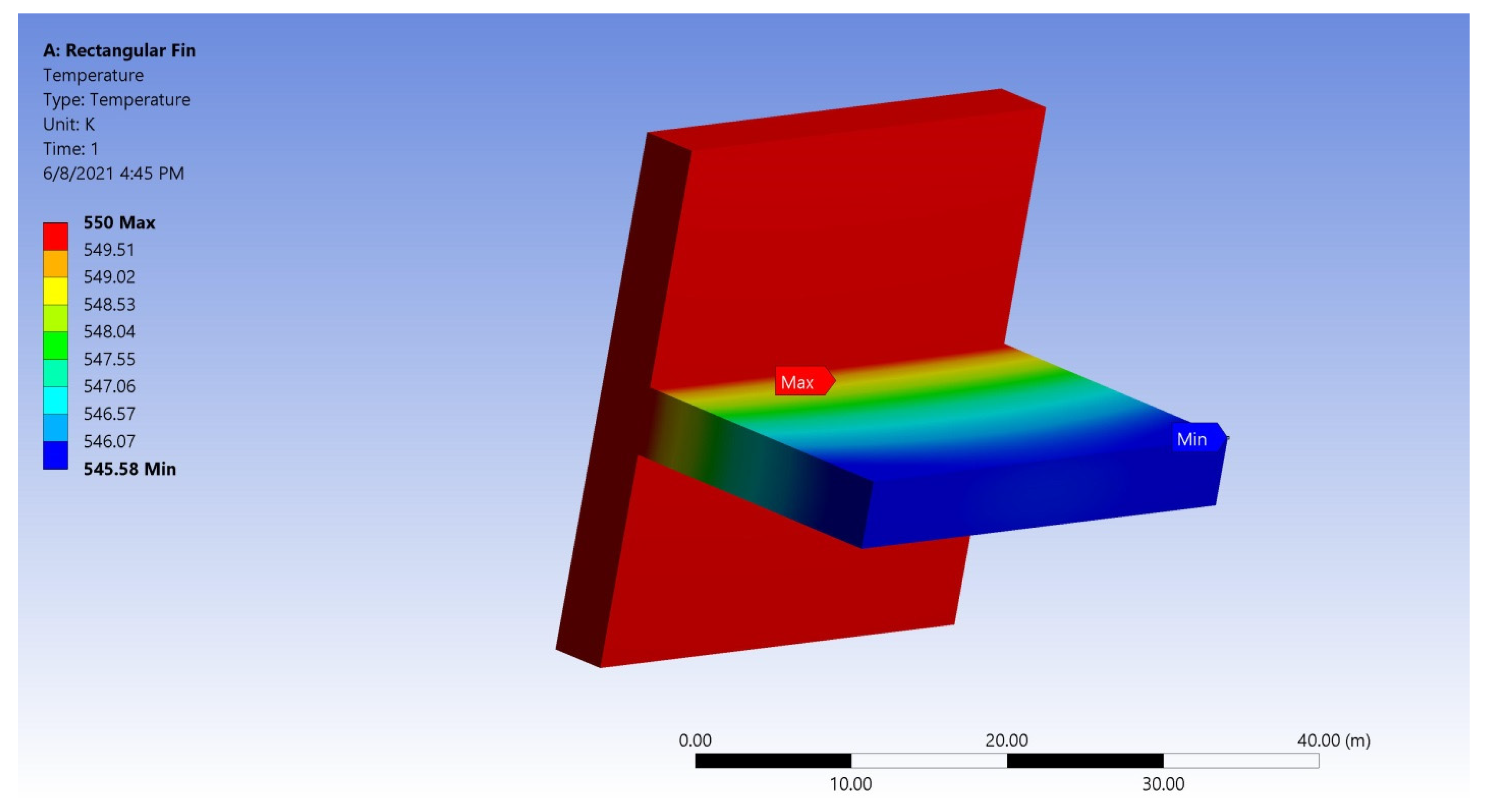
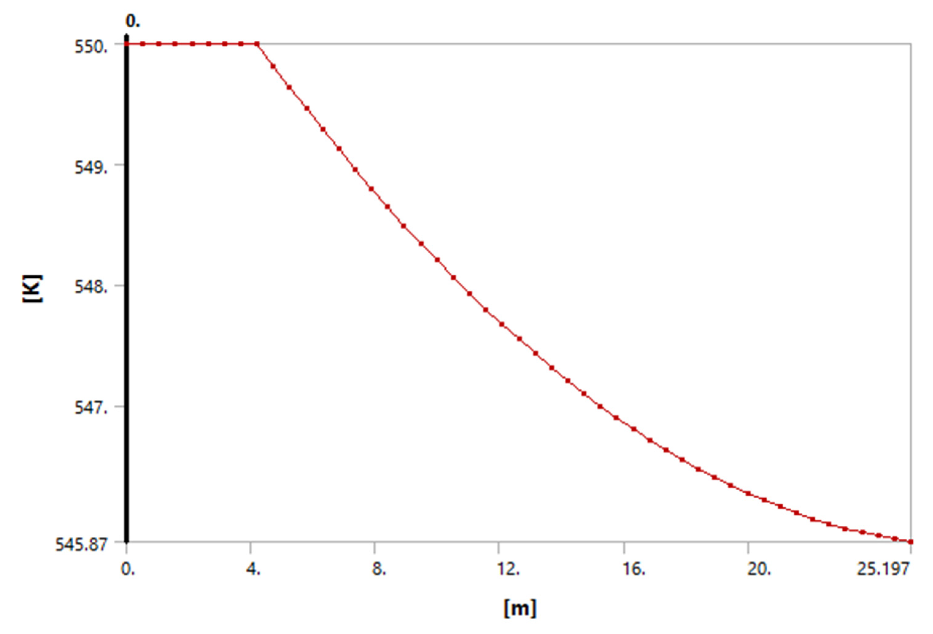
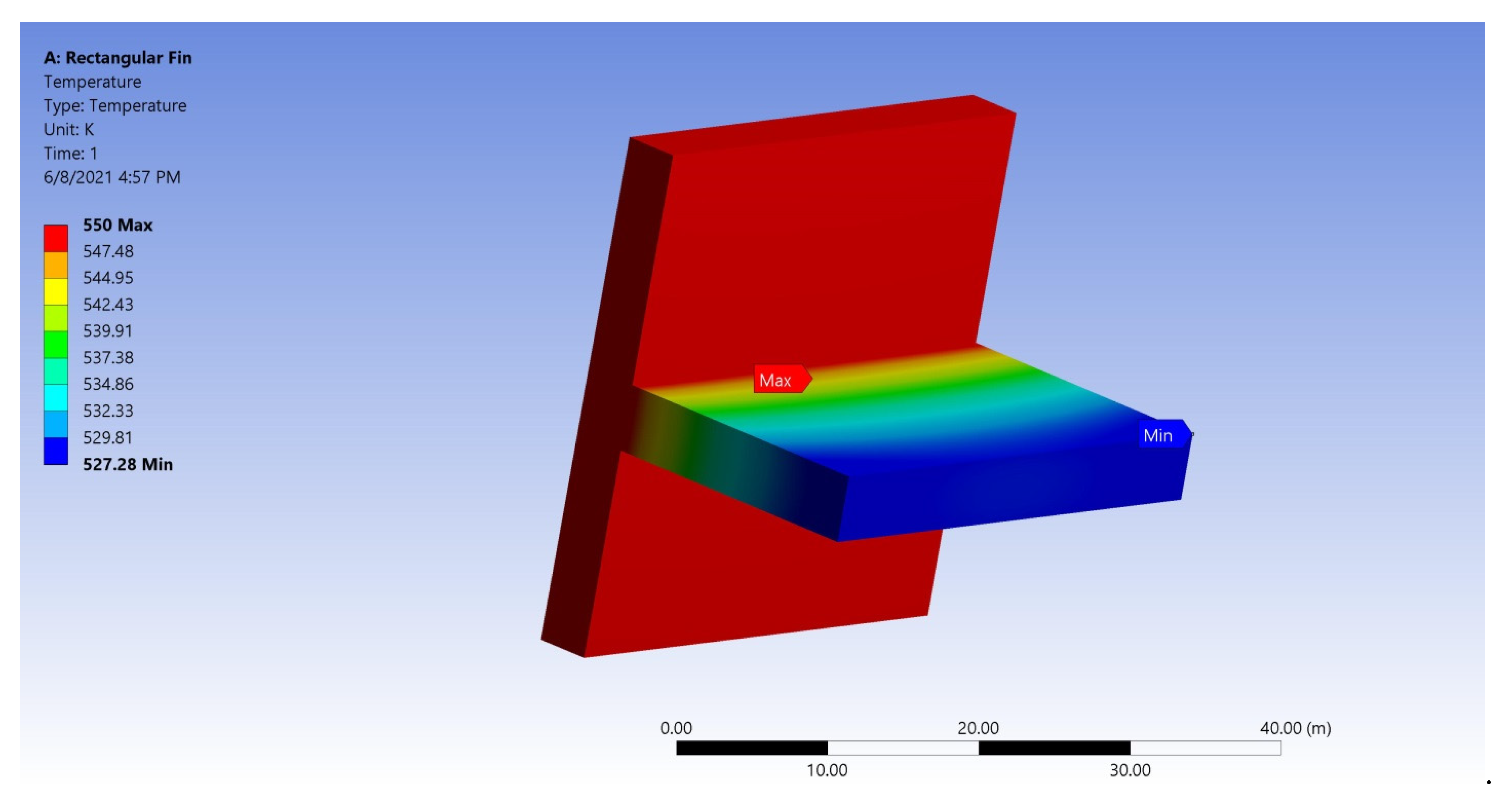
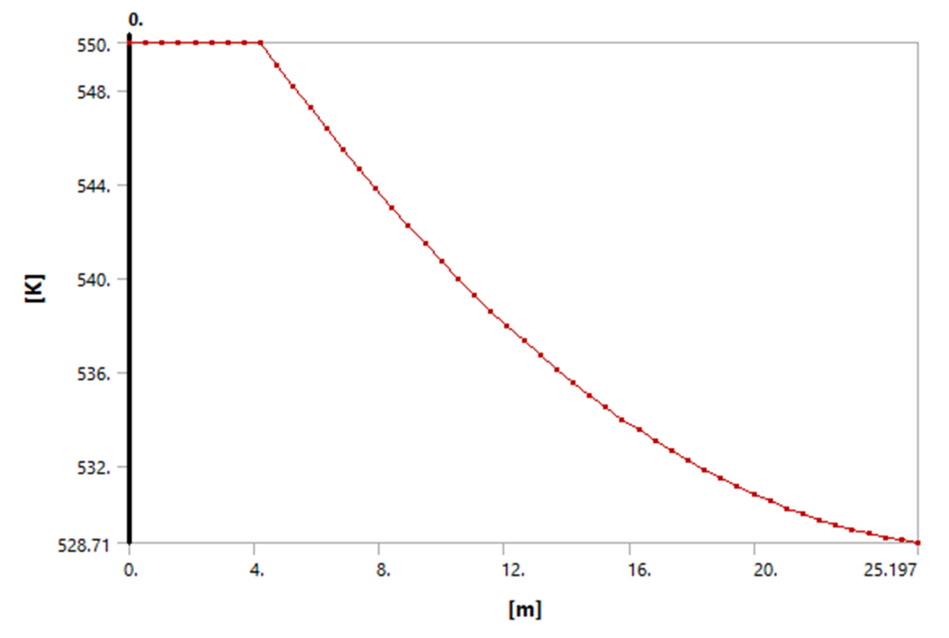
7. Inspecting the Thermal Behavior of a Longitudinal Fin Using ANSYS

ANSYS is a general-purpose software package that affords a cost-effective approach to inspecting the better performance of mechanical and fluid models or processes in a virtual environment. This software implements governing equations for corresponding problems to study the behavior of problems and solves them efficiently. The obtained results are presented in tabular or graphical forms.

To inspect the thermal behavior, a longitudinal fin is modeled with the following assumptions:

• Since aluminum is an excellent thermal and electrical conductor, Aluminum Alloy 6061 (AA 6061) and Cast Iron with constant thermal conductivity 300 $\mathrm{W}/\mathrm{m} \mathrm{K}$ and 55 $\mathrm{W}/\mathrm{m} \mathrm{K}$ are taken as fin materials.
• One-dimensional heat conduction is considered along the longitudinal direction.
• The convective heat transfer coefficient (39.9 ${\mathrm{W}/\mathrm{m}}^2 \mathrm{K}$) is considered over the complete fin surface.
• The temperature at the fin base is 550 K, and the ambient temperature is 283 K.

The temperature distribution of a longitudinal fin made up of AA 6061, and Cast Iron can be assessed with an ANSYS workbench. For the longitudinal fin made up of AA 6061, the maximum temperature at the prime surface is 550 K. By contrast, the minimum temperature is 545.58 K observed at the end of the fin, and 548.9 K is the average temperature. From this analysis, it is found that the extreme temperature of 550 K is at the source, and the minimum temperature of 527.28 K will be at the end of the fin for the fin of material Cast Iron. It is also noticed that the average temperature through the fin is 544.33 K. The temperature gradually decreases from one end to another end, that is from base to tip end based on the given heat transfer coefficient as shown in Figure 17, Figure 18, Figure 19 and Figure 20.

8. Final Remarks

The temperature dispersal of a longitudinal rectangular fin with exponential temperature-dependent heat transfer coefficient and internal heat generation is inspected by considering exponential temperature-dependent $k^{*}\left(T\right)$ with the aid of the DTM-Pade approximant. The significant results of the present scrutiny are as follows:

• Enhancement in the scale of thermo-geometric parameters reduces temperature dispersal in a fin for both cases.
• Temperature distribution enriches for a larger magnitude of thermal conductivity parameter in the case of linear temperature-dependent thermal conductivity.
• Larger values of the internal heat generation and heat transfer parameter upsurge the thermal distribution in both cases.
• The efficiency of a fin varies with prescribed non-dimensional thermal parameters under internal heat generation.
• The thermal distribution of a longitudinal fin is studied using ANSYS software by considering the material of the fin body as AA 6061 and Cast Iron. The temperature is higher at the base, decreasing monotonically towards the fin tip.
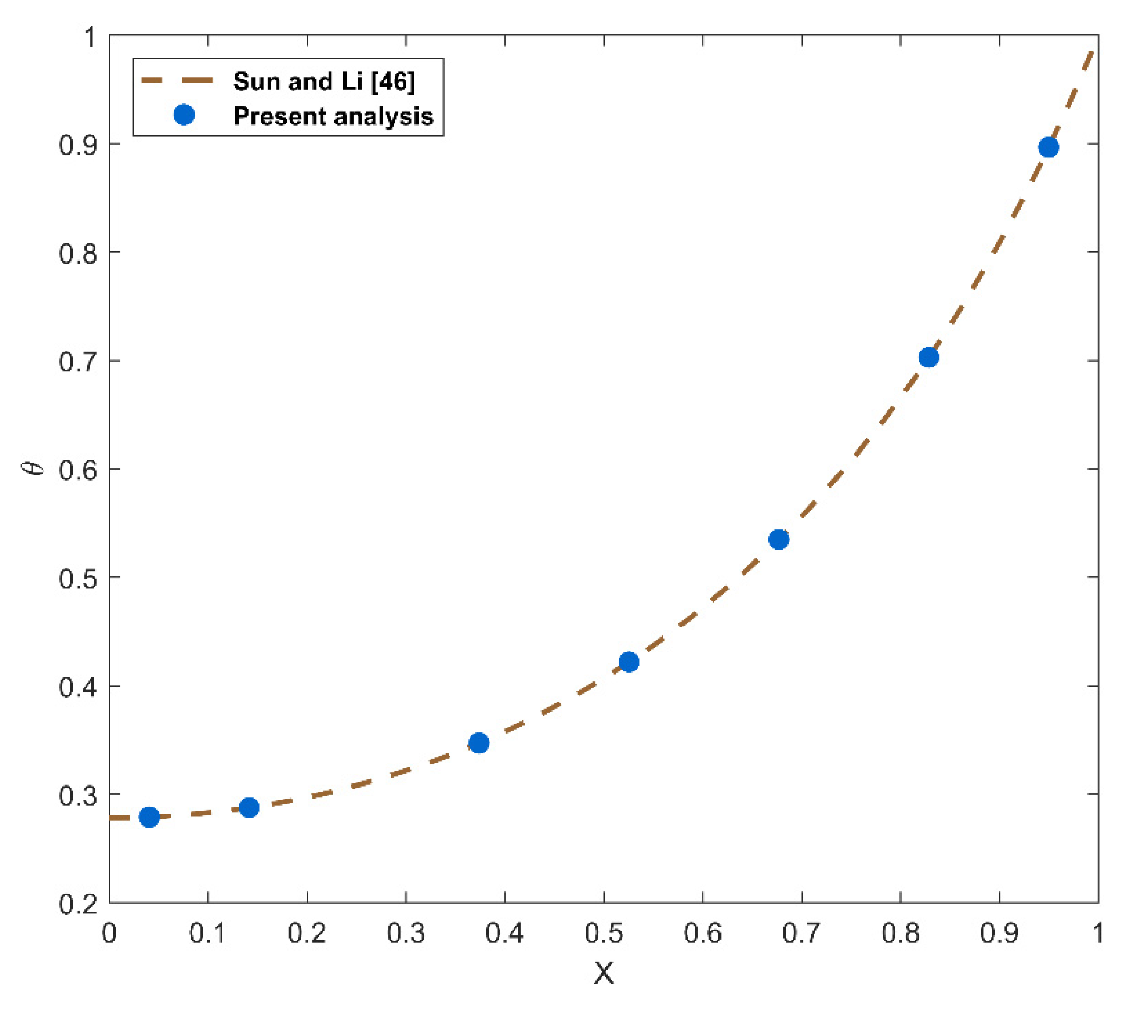
• The analytical solution and numerical results obtained by the DTM-Pade approximant afford higher accuracy than other techniques.

References

1. Khan, S.U.; Tlili, I. Significance of Activation Energy and Effective Prandtl Number in Accelerated Flow of Jeffrey Nanoparticles With Gyrotactic Microorganisms. J. Energy Resour. Technol. 2020, 142, 112101. [Google Scholar] [CrossRef]
2. Hosseinzadeh, K.; Moghaddam, M.E.; Asadi, A.; Mogharrebi, A.; Ganji, D. Effect of internal fins along with Hybrid Nano-Particles on solid process in star shape triplex Latent Heat Thermal Energy Storage System by numerical simulation. Renew. Energy 2020, 154, 497–507. [Google Scholar] [CrossRef]
3. Khan, S.U.; Al-Khaled, K.; Aldabesh, A.; Awais, M.; Tlili, I. Bioconvection flow in accelerated couple stress nanoparticles with activation energy: Bio-fuel applications. Sci. Rep. 2021, 11, 3331. [Google Scholar] [CrossRef] [PubMed]
4. Hamid, A.; Kumar, R.N.; Gowda, R.J.P.; Khan, S.U.; Khan, M.I.; Prasannakumara, B.C.; Muhammad, T. Impact of Hall current and homogenous–heterogenous reactions on MHD flow of GO-MoS2/water (H2O)-ethylene glycol (C2H6O2) hybrid nanofluid past a vertical stretching surface. Waves Random Complex Media 2021, 1–18. [Google Scholar] [CrossRef]
5. Khan, M.I.; Qayyum, S.; Chu, Y.-M.; Khan, N.B.; Kadry, S. Transportation of Marangoni convection and irregular heat source in entropy optimized dissipative flow. Int. Commun. Heat Mass Transf. 2021, 120, 105031. [Google Scholar] [CrossRef]
6. Madhukesh, J.K.; Kumar, R.N.; Gowda, R.J.P.; Prasannakumara, B.C.; Ramesh, G.K.; Khan, M.I.; Khan, S.U.; Chu, Y.-M. Numerical simulation of AA7072-AA7075/water-based hybrid nanofluid flow over a curved stretching sheet with Newtonian heating: A non-Fourier heat flux model approach. J. Mol. Liq. 2021, 335, 116103. [Google Scholar] [CrossRef]
7. Raza, A.; Khan, S.U.; Al-Khaled, K.; Khan, M.I.; Haq, A.U.; Alotaibi, F.; Allah, A.M.A.; Qayyum, S. A fractional model for the kerosene oil and water-based Casson nanofluid with inclined magnetic force. Chem. Phys. Lett. 2021, 787, 139277. [Google Scholar] [CrossRef]
8. Hosseinzadeh, K.; Mogharrebi, A.; Asadi, A.; Paikar, M.; Ganji, D. Effect of fin and hybrid nano-particles on solid process in hexagonal triplex Latent Heat Thermal Energy Storage System. J. Mol. Liq. 2020, 300, 112347. [Google Scholar] [CrossRef]
9. Hosseinzadeh, K.; Montazer, E.; Shafii, M.B.; Ganji, A. Solidification enhancement in triplex thermal energy storage system via triplets fins configuration and hybrid nanoparticles. J. Energy Storage 2021, 34, 102177. [Google Scholar] [CrossRef]
10. Kundu, B. Performance and optimum design analysis of longitudinal and pin fins with simultaneous heat and mass transfer: Unified and comparative investigations. Appl. Therm. Eng. 2007, 27, 976–987. [Google Scholar] [CrossRef]
11. Aziz, A.; Bouaziz, M. A least squares method for a longitudinal fin with temperature dependent internal heat generation and thermal conductivity. Energy Convers. Manag. 2011, 52, 2876–2882. [Google Scholar] [CrossRef]
12. Najafabadi, M.F.; Rostami, H.T.; Hosseinzadeh, K.; Ganji, D.D. Thermal analysis of a moving fin using the radial basis function approximation. Heat Transf. 2021, 50, 7553–7567. [Google Scholar] [CrossRef]
13. Sowmya, G.; Sarris, I.E.; Vishalakshi, C.S.; Kumar, R.S.V.; Prasannakumara, B.C. Analysis of Transient Thermal Distribution in a Convective–Radiative Moving Rod Using Two-Dimensional Differential Transform Method with Multivariate Pade Approximant. Symmetry 2021, 13, 1793. [Google Scholar] [CrossRef]
14. Sowmya, G.; Kumar, R.S.V.; Alsulami, M.D.; Prasannakumara, B.C. Thermal stress and temperature distribution of an annular fin with variable temperature-dependent thermal properties and magnetic field using DTM-Pade approximant. Waves Random Complex Media 2022, 1–29. [Google Scholar] [CrossRef]
15. Zhang, H.J.; Sun, K.F. Conduction from Longitudinal Fin of Rectangular Profile with Exponential Vary Heat Transfer Coefficient. Adv. Mater. Res. 2012, 614–615, 311–314. [Google Scholar]
16. Buikis, A.; Pagodkina, I. Comparison of Analytical and Numerical Solutions for a Two-Dimensinal Longitudal Fin of Rectangular Profile. Latv. J. Phys. Tech. Sci. 1996. [Google Scholar] [CrossRef]
17. Kezzar, M.; Tabet, I.; Eid, M.R. A new analytical solution of longitudinal fin with variable heat generation and thermal conductivity using DRA. Eur. Phys. J. Plus 2020, 135, 120. [Google Scholar] [CrossRef]
18. Wang, F.; Kumar, R.V.; Sowmya, G.; El-Zahar, E.R.; Prasannakumara, B.; Khan, M.I.; Khan, S.U.; Malik, M.; Xia, W.-F. LSM and DTM-Pade approximation for the combined impacts of convective and radiative heat transfer on an inclined porous longitudinal fin. Case Stud. Therm. Eng. 2022, 101846. [Google Scholar] [CrossRef]
19. Alhejaili, W.; Kumar, R.V.; El-Zahar, E.R.; Sowmya, G.; Prasannakumara, B.; Khan, M.I.; Yogeesha, K.; Qayyum, S. Analytical solution for temperature equation of a fin problem with variable temperature-dependent thermal properties: Application of LSM and DTM-Pade approximant. Chem. Phys. Lett. 2022, 793, 139409. [Google Scholar] [CrossRef]
20. Torabi, M.; Aziz, A.; Zhang, K. A comparative study of longitudinal fins of rectangular, trapezoidal and concave parabolic profiles with multiple nonlinearities. Energy 2013, 51, 243–256. [Google Scholar] [CrossRef]
21. Mallick, A.; Ghosal, S.; Sarkar, P.K.; Ranjan, R. Homotopy Perturbation Method for Thermal Stresses in an AnnularFinwith Variable Thermal Conductivity. J. Therm. Stress. 2014, 38, 110–132. [Google Scholar] [CrossRef]
22. Atouei, S.; Hosseinzadeh, K.; Hatami, M.; Ghasemi, S.E.; Sahebi, S.; Ganji, D. Heat transfer study on convective–radiative semi-spherical fins with temperature-dependent properties and heat generation using efficient computational methods. Appl. Therm. Eng. 2015, 89, 299–305. [Google Scholar] [CrossRef]
23. Turkyilmazoglu, M. Heat transfer from moving exponential fins exposed to heat generation. Int. J. Heat Mass Transf. 2018, 116, 346–351. [Google Scholar] [CrossRef]
24. Padmanabhan, S.; Thiagarajan, S.; Kumar, A.D.R.; Prabhakaran, D.; Raju, M. Investigation of temperature distribution of fin profiles using analytical and CFD analysis. Mater. Today: Proc. 2021, 44, 3550–3556. [Google Scholar] [CrossRef]
25. Hosseinzadeh, S.; Hasibi, A.; Ganji, D. Thermal analysis of moving porous fin wetted by hybrid nanofluid with trapezoidal, concave parabolic and convex cross sections. Case Stud. Therm. Eng. 2022, 30, 101757. [Google Scholar] [CrossRef]
26. Minkler, W.S.; Rouleau, W.T. The Effects of Internal Heat Generation on Heat Transfer in Thin Fins. Nucl. Sci. Eng. 1960, 7, 400–406. [Google Scholar] [CrossRef]
27. Venkitesh, V.; Mallick, A. Thermal analysis of a convective–conductive–radiative annular porous fin with variable thermal parameters and internal heat generation. J. Therm. Anal. 2020, 147, 1519–1533. [Google Scholar] [CrossRef]
28. Majhi, T.; Kundu, B. New Approach for Determining Fin Performances of an Annular Disc Fin with Internal Heat Generation. In Advances in Mechanical Engineering; Springer: Singapore, 2020; pp. 1033–1043. [Google Scholar] [CrossRef]
29. Das, R.; Kundu, B. Prediction of Heat-Generation and Electromagnetic Parameters from Temperature Response in Porous Fins. J. Thermophys. Heat Transf. 2021, 35, 761–769. [Google Scholar] [CrossRef]
30. Jayaprakash, M.; Alzahrani, H.A.; Sowmya, G.; Kumar, R.V.; Malik, M.; Alsaiari, A.; Prasannakumara, B. Thermal distribution through a moving longitudinal trapezoidal fin with variable temperature-dependent thermal properties using DTM-Pade approximant. Case Stud. Therm. Eng. 2021, 28, 101697. [Google Scholar] [CrossRef]
31. Zhou, J.K. Differential Transformation and Its Applications for Electrical Circuits; Huazhong University Press: Wuhan, China, 1986. [Google Scholar]
32. Kundu, B.; Lee, K.-S. Analytical tools for calculating the maximum heat transfer of annular stepped fins with internal heat generation and radiation effects. Energy 2014, 76, 733–748. [Google Scholar] [CrossRef]
33. Moradi, A.; Hayat, T.; Alsaedi, A. Convection-radiation thermal analysis of triangular porous fins with temperature-dependent thermal conductivity by DTM. Energy Convers. Manag. 2014, 77, 70–77. [Google Scholar] [CrossRef]
34. Christopher, A.J.; Magesh, N.; Gowda, R.J.P.; Kumar, R.N.; Kumar, R.S.V. Hybrid nanofluid flow over a stretched cylinder with the impact of homogeneous–heterogeneous reactions and Cattaneo–Christov heat flux: Series solution and numerical simulation. Heat Transf. 2021, 50, 3800–3821. [Google Scholar] [CrossRef]
35. Kundu, B.; Yook, S.-J. An accurate approach for thermal analysis of porous longitudinal, spine and radial fins with all nonlinearity effects—Analytical and unified assessment. Appl. Math. Comput. 2021, 402, 126124. [Google Scholar] [CrossRef]
36. Baker, G.A., Jr. Essentials of Padé Approximants; Academic Press: New York, NY, USA, 1975; 317p, ISBN 0-12-074885-X. [Google Scholar]
37. Baker, G.A.; Graves-Morris, P.R. Padé Approximants: Extensions and Applications; Addison-Wesley: Boston, MA, USA, 1981; Volume 2. [Google Scholar]
38. Rashidi, M.M.; Keimanesh, M. Using Differential Transform Method and Padé Approximant for Solving MHD Flow in a Laminar Liquid Film from a Horizontal Stretching Surface. Math. Probl. Eng. 2010, 2010, 491319. [Google Scholar] [CrossRef]
39. Rashidi, M.M.; Laraqi, N.; Sadri, S.M. A novel analytical solution of mixed convection about an inclined flat plate embedded in a porous medium using the DTM-Padé. Int. J. Therm. Sci. 2010, 49, 2405–2412. [Google Scholar] [CrossRef]
40. Saha, D.; Sengupta, S. Dual DTM-Padé approximations on free convection MHD mass transfer flow of nanofluid through a stretching sheet in presence of Soret and Dufour Phenomena. WSEAS Trans. Fluid Mech. 2020, 15, 23–40. [Google Scholar] [CrossRef]
41. Moradi, A.; Ahmadikia, H. Investigation of Effect Thermal Conductivity on Straight Fin Performance with DTM. Int. J. Eng. Appl. Sci. 2011, 3, 42–54. [Google Scholar]
42. Jawad, A.J.M. Differential Transformation Method for Solving Nonlinear Heat Transfer Equations. Al-Rafidain Univ. Coll. Sci. 2013, 32, 180–194. [Google Scholar]
43. Boyd, J.P. Padé approximant algorithm for solving nonlinear ordinary differential equation boundary value problems on an unbounded domain. Comput. Phys. 1997, 11, 299. [Google Scholar] [CrossRef]
44. Ismail, T.; Kezzar, M.; Touafe, K.; Bellel, N.; Gherieb, S.; Khelifa, A.; Adouane, M. Adomian Decomposition Method And Padé Approximation To Determine Fin Efficiency Of Convective Solar Air Collector In Straight Fins. Int. J. Math. Model. Comput. 2015, 5, 335–346. [Google Scholar]
45. Languri, E.M.; Ganji, D.D.; Jamshidi, N. Variational Iteration and Homotopy perturbation methods for fin efficiency of convective straight fins with temperature dependent thermal conductivity. In Proceedings of the 5th WSEAS international conference On FLUID MECHANICS (Fluids 08), Acapulco, Mexico, 25–27 January 2008; Volume 25. [Google Scholar]
46. Sun, S.-W.; Li, X.-F. Exact solution of the nonlinear fin problem with exponentially temperature-dependent thermal conductivity and heat transfer coefficient. Pramana 2020, 94, 94. [Google Scholar] [CrossRef]
Figure 1. Schematic representation of a longitudinal fin.
Symmetry 14 00690 g001
Figure 2. Validation of the present analysis with existing work (Sun and Li [46]) for a = 1 , b = 0 , α = 1.6 , Q = γ = 0 .
Symmetry 14 00690 g002
Figure 3. Impact of α on θ .
Symmetry 14 00690 g003
Figure 4. Impact of γ on θ .
Symmetry 14 00690 g004
Figure 5. Impact of Q on θ .
Symmetry 14 00690 g005
Figure 6. Impact of a on θ .
Symmetry 14 00690 g006
Figure 7. Impact of b on θ .
Symmetry 14 00690 g007
Figure 8. Influence of α on fin efficiency.
Symmetry 14 00690 g008
Figure 9. Impact of Q on fin efficiency.
Symmetry 14 00690 g009
Figure 10. Impact of b on fin efficiency.
Symmetry 14 00690 g010
Figure 11. Impact of α on θ .
Symmetry 14 00690 g011
Figure 12. Impact of γ on θ .
Symmetry 14 00690 g012
Figure 13. Impact of Q on θ .
Symmetry 14 00690 g013
Figure 14. Impact of β on θ .
Symmetry 14 00690 g014
Figure 15. Impact of b on θ .
Symmetry 14 00690 g015
Figure 16. Comparing the temperature distribution of a fin with exponential temperature-dependent and linearly temperature-dependent thermal conductivity.
Symmetry 14 00690 g016
Figure 17. Temperature distribution for Aluminum Alloy 6061.
Symmetry 14 00690 g017
Figure 18. Temperature varying along the length of the fin for Aluminum Alloy 6061.
Symmetry 14 00690 g018
Figure 19. Temperature distribution for Cast Iron.
Symmetry 14 00690 g019
Figure 20. Temperature varying along the length of the fin for Cast Iron.
Symmetry 14 00690 g020