A Method for the Design of Bicomplex Orthogonal DSP Algorithms for Applications in Intelligent Radio Access Networks

Abstract

In this paper, a new method for designing orthogonal bicomplex digital signal processing (DSP) algorithms is developed. In contrast to those previously reported on, the method proposed is universal, since it is not affected by the order or the type of the real digital processing algorithm employed as a prototype. The method is based on a transformation starting with either real or complex orthogonal DSP algorithms represented in the z-domain, and transforming them into orthogonal bicomplex algorithms. The proposed new method is applied in the design of bilinear orthogonal bicomplex DSP systems with a canonical number of elements, the main advantage of which is that the order of the digital system is reduced by a factor of four. As well as being canonical, the orthogonal bicomplex digital systems are also symmetrical structures, as a result of which they offer parallelism and subsequent unification. It is experimentally shown that bicomplex orthogonal DSP algorithms acquire the properties of the initial algorithm prototype, irrespective of whether it is real or complex. Since the new design method is universally applicable, it can be used to develop bicomplex orthogonal digital algorithms of any order and type. Being simple, canonical, and symmetrical—and, thus, leading to lower equipment cost, reduced complexity, and higher energy efficiency—these structures may well be appropriate for the enhancement of the implementation of intelligent algorithms in next-generation radio access networks.

1. Introduction

The first nine numerical systems based on real numbers have already been defined as objects in mathematics. These are part of Cayley–Dickson algebra, and have different dimensions based on 2ⁿ, where n denotes the number of imaginary units in the particular numerical system. For n = 0, the one-dimensional (1D) real numbers ( —Real) are obtained. For n = 1 we get the two-dimensional (2D) complex numbers ( —Complex). Thereafter, n = 2 gives rise to the four-dimensional (4D) quaternions ( —Quaternions). According to the logic of doubling the dimensions on which Cayley–Dickson algebra is built, after quaternions the so-called 8D octonions (𝕆—Octonions) can be obtained, followed by 16D sedenions, 32D pathions, 64D chingons, 128D routons, and 256D voudons. All numerical systems with a dimension higher than the second are called hypercomplex numbers. The value of the square of the imaginary units and the interdependencies they obey determine the different types of arithmetic contained in each numerical system. For example, 1D numbers can be integers or fractions, while 2D numbers can be classic complex numbers, hyperbolic numbers, or dual-complex numbers.

Most of the number systems listed above are still the subject of study solely in purely theoretical sciences, such as theoretical mathematics and theoretical physics. Only the first four number systems ( , , , and 𝕆) have found practical applications so far. In addition to numerous practical solutions based on real or complex numbers, intensive research based on 4D and 8D numbers has been conducted over the past three or four decades. The applications of the mathematically complicated but very powerful 4D hypercomplex numbers are both copious and ubiquitous. Among them are areas such as robotics, space technology, telemedicine, air and sea navigation, seismology, meteorology, microbiology, geology, and many others. Octonions are not as well studied as complex numbers and quaternions; hence, they have not yet been widely used in practice. Some current areas of application of 8D octonions include string theory, special relativity theory, quantum logic, and the entropy and thermodynamics of black holes.

The mathematical theory of 4D numbers with commutative algebra proves to be suitable for the development and improvement of many advanced telecommunication technologies. Among the applications in telecommunications for which commutative 4D hypercomplex digital processing is an appropriate and elegant tool for the description, analysis, and optimization of systems and processes, are audio and speech signal processing [1,2], digital colour image processing [3], measurement and suppression of noise and interference [4], video signal processing and image recognition, computer vision, facial recognition and neural networks [5,6], data compression, coding and information security [7], radar, sonar, and sensory processing [8], motion control systems, location and spatial orientation, reconstruction and localization of three-dimensional objects [9,10], etc.

To ensure non-interruptive service provision to the users together with the required quality of service (QoS), next-generation communication networks (NGNs) and access networks (ANs) give rise to many new scientific challenges. For example, ultradense networks (UDNs), which integrate heterogeneous access nodes in ultradense deployment scenarios, face a number of challenges, such as efficient spectrum and energy utilization, resource and mobility management, power and interference management, implementation of beamforming, QoS-based resource optimization, etc. To meet such challenges, the design of the access nodes should include programmable, virtualized, flexible, intelligent, and energy-efficient approaches, most of them depending on appropriate DSP algorithms. It is DSP algorithms that are applied to process and analyse data; for spectrum sensing; for interference suppression; to amplify, extract, or compensate for signal imperfections; to split signals into subsignals; to limit or select frequency bands or channels; to align communication channels, etc.

Another challenge in NGNs is the implementation of intelligence in the nodes of the AN. In the last few years, the concept of openness and intelligence of the radio access network (RAN) has been introduced. The idea behind this is to evolve current RAN architectures and deploy virtualized and fully interoperable next-generation wireless access based on two fundamental principles: openness—utilizing open software—and intelligence, implemented in the RAN architecture [11]. The design framework of such architectures enables an open and intelligent RAN, founded on the principles of openness and intelligence. The agile and open structure of such an intelligent RAN enables the deployment of a diverse range of novel usage scenarios, such as low-cost radio access networks, QoS-based resource optimization, massive multiple-input multiple-output (MIMO) optimization, context-based dynamic handover management for vehicle-to-everything (V2X), flight-path-based dynamic unmanned aerial vehicle (UAV) resource allocation, radio resource allocation for UAV applications, and RAN sharing. A software-defined, unbundled, programmable, flexible, and intelligent RAN architecture can address the increasing demands related to mobile broadband and ultralow latency [12,13].

Major elements included in the architecture of open and intelligent RANs include the so-called radio intelligent controllers (RICs). The RICs usually implement a control loop with a high timing constraint (as little as 10 ms), executing operationally demanding functions, including load balancing, optimization actions and policies, radio resource management, interference detection and mitigation, etc.

These units are also aimed to support baseband signal processing and data analytics so as to enable embedding artificial intelligence (AI) and machine learning (ML) in the nodes [14]. Thus, we consider that it is important in such RICs to utilize the advantages of the implementation of appropriate bicomplex DSP algorithms, since intelligent RANs will operate in scenarios that deal with heterogeneous and densely deployed nodes, together with larger bandwidths and higher data rates, addressing the challenge of embedding AI/ML models.

Depending on the numerical system used, DSP algorithms can be classified as real, complex, or hypercomplex. While the first DSP algorithms developed were real, interest among the scientific community in complex digital signal processing was also emerging at around the same time [15]. It is considered that the concept of complex digital processing belongs to Crystal and Ehrman, and was set out in their work in 1968 [16]. This publication, like many others, demonstrates the higher efficiency of complex DSP compared to real DSP [17,18,19]. Researchers are still very interested in complex digital signal processing, which makes complex digital algorithms a well-developed scientific field at present.

The scientific research shows that only those 4D numbers with commutative multiplication are applicable to DSP systems. The precise name of the digital algorithms using commutative 4D hypercomplex coefficients is bicomplex, but they are often referred to by the more general name hypercomplex. Despite the more complicated math, bicomplex DSP algorithms have become more widely studied in recent years due to their advantages in processing signals represented by real, complex, or bicomplex numbers [20]. The fourfold reduction in the order of a bicomplex algorithm compared to a real one, together with the potential for parallelism and the significant simplification of the digital implementation due to the mirror symmetry of the DSP structure, makes bicomplex DSP algorithms efficient and attractive for various applications.

A number of methods for designing bicomplex digital algorithms have been developed, but none of them is universally applicable. Most of these methods are related to specific types of digital structures, narrowing the areas for their application and making them non-universal [21,22]. Choosing the most suitable digital implementation for a given application is very important, and is directly related to the efficiency of the digital algorithm. Logically, the use of a limited number of elements will lead to more economical, cheaper, and faster processing. Hence, the choice of the implementation is crucial as regards the efficiency of digital processing. Furthermore, it is important that any designed DSP algorithm should provide computational efficiency, low sensitivity, and reduced complexity. A number of scientific publications deal with these complicated optimization problems [22,23,24].

Many 4D DSP algorithms are associated with the beneficial property of orthogonality. In order to process an orthogonal hypercomplex signal, such as an ordered pair of analytical signals, an orthogonal hypercomplex digital algorithm is needed. Over the past 25 years or so, numerous methods for designing such algorithms have been put forward in the literature [21,25], most of which were developed for specific digital structures, thus rendering them non-universal. In [26,27], a design procedure for orthogonal hypercomplex DSP algorithms—based on the concept that an orthogonal algorithm with real coefficients is expanded into one with hypercomplex coefficients through the use of an “orthogonal polynomial expansion”—is proposed. However, this has a drawback in that the design procedure is based on a real all-pass structure, which is not capable of processing a pair of orthogonal complex signals. Orthogonal transforms—for example, the quaternion polar harmonic transform (QPHT) [28] and quaternion polar linear canonical transform (QPLCT) [29]—are employed in the improvement of image representation capability and numerical stability.

This paper describes a new design method for orthogonal bicomplex DSP algorithms. This method is appropriate for any digital structure of any order, and is developed in the complex frequency z-domain. The operation of the method ise shown by a numerical example, and the designed orthogonal bicomplex DSP algorithm is analysed.

The rest of the paper is arranged as follows: 4D numerical systems applicable to DSP are introduced in Section 2. Section 3 outlines the main properties of commutative bicomplex numbers—in particular the so-called reduced biquaternions (RBQs). A new design procedure for orthogonal bicomplex DSP algorithms is presented in Section 4. In Section 5, a numerical example shows the applicability of the proposed method. Section 6 concludes the paper.

2. 4D Numerical Systems Applicable to DSP

In 1843, just a few years after the complete development of the algebra of complex 2D numbers, the Irish mathematician Sir William R. Hamilton defined quaternions as a generalization of complex numbers. Named after him, the Hamilton quaternions were the first 4D hypercomplex numbers to be discovered.

The quaternion is an ordered sequence of four real numbers a, b, c, and d—one scalar a, and one three-dimensional vector (b, c, d). A quaternion may be represented in hypercomplex form as follows:

$$\begin{array}{c}Q=a+b{i}_1+c{i}_2+d{i}_3=\\ =Q_S+Q_V,\end{array}$$

(1)

where Q_S = a and Q_V = bi₁ + ci₂ + di₃ are called the scalar and vector parts of the quaternion, respectively, while i₁, i₂, and i₃ are mutually orthogonal imaginary units whose squares, in general, can be equal to −1, +1, or 0. Depending on these numerical values, as well as the multiplication rules that i₁, i₂, and i₃ comply with, different types of quaternions are defined, such as pseudo-quaternions, degenerate quaternions, and degenerate pseudo-quaternions [30]. These and many others belong to the large family of 4D hypercomplex numbers. The most commonly used are Hamilton’s quaternions, which are often simply called quaternions. The three imaginary units, known as the orthogonal basis of a quaternion, obey the following rules:

$$\begin{array}{c}{i}_1^2=i_2^2=i_3^2=i_1{i}_2{i}_3=-1;\\ i_1{i}_2=i_3;\hspace{1em}{i}_2{i}_1=-i_3;\\ i_2{i}_3=i_1;\hspace{1em}{i}_3{i}_2=-i_1;\\ i_3{i}_1=i_2;\hspace{1em}{i}_1{i}_3=-i_2.\end{array}$$

(2)

The theory behind Hamilton’s quaternions incorporates the concept of vectors in space. A quaternion converts one vector into another vector by multiplication, which is closely related to the nature of three-dimensional space. Quaternions are used both in purely theoretical mathematics and in applied mathematics and physics, mostly for the efficient calculation of spatial rotation.

Regrettably, Hamilton’s quaternions are not applicable to DSP systems because their multiplication is associative rather than commutative, and no digital processing algorithms based on noncommutative algebra have yet been developed. The need to find a solution to this problem was the main driving force behind the discovery of the so-called commutative bicomplex numbers and the associated theory.

A bicomplex number BC is defined as an ordered pair of complex numbers C₁ and C₂, with specifically defined properties, as follows [31]:

$$BC=\left(a+b{i}_1\right)+i_2\left(c+d{i}_1\right)=C_1+i_2{C}_2=\left(C_1,C_2\right),$$

(3)

where i₁² = {−1, 0, +1}, i₂² = {−1, 0, +1} as well as i₁,i₂ and i₁i₂ are uncorrelated and commutative (i₁i₂ = i₂i₁) imaginary units. Therefore, bicomplex numbers are complex numbers with complex coefficients—hence, the name bicomplex.

The set {1, i₁, i₂, i₃}, where i₃ = i₁i₂ = i₂i₁, is the basis of a bicomplex number, which can also be represented in hypercomplex form as a 4D number with real coefficients, as follows:

$$BC=a+b{i}_1+c{i}_2+d{i}_1{i}_2.$$

(4)

Depending on the values of the squares of the imaginary units, different bicomplex numbers are defined, and some of these are presented in

Table 1. Different types of bicomplex numbers.

Bicomplex Numbers	i1	i2	i3= i1i2 = i2i1
Tessarines	$i_1^2=-1$	$\begin{array}{l}{i}_2^2=+1\\ i_2\ne \pm 1\end{array}$	$i_3^2=+1$
Reduced biquaternions	$i_1^2=-1$	$i_2^2=-1$	$i_3^2=+1$
Complex hyperbolic numbers	$i_1^2=-1$	$\begin{array}{l}{i}_2^2=+1\\ i_2\ne \pm 1\end{array}$	$i_3^2=-1$
Hyperbolic complex numbers	$\begin{array}{l}{i}_1^2=+1\\ i_1\ne \pm 1\end{array}$	$i_2^2=-1$	$i_3^2=-1$
Hyperbolic dual numbers	$\begin{array}{l}{i}_1^2=+1\\ i_1\ne \pm 1\end{array}$	$\begin{array}{l}{i}_2^2=0\\ i_2\ne 0\end{array}$	$\begin{array}{l}{i}_2{i}_3=0\\ i_1{i}_3=i_2\end{array}$
Dual hyperbolic numbers	$\begin{array}{l}{i}_1^2=0\\ i_1\ne 0\end{array}$	$\begin{array}{l}{i}_2^2=+1\\ i_2\ne \pm 1\end{array}$	$\begin{array}{l}{i}_2{i}_3=i_1\\ i_1{i}_3=0\end{array}$
Hyper-dual numbers	$\begin{array}{l}{i}_1^2=0\\ i_1\ne 0\end{array}$	$\begin{array}{l}{i}_2^2=0\\ i_2\ne 0\end{array}$	$\begin{array}{l}{i}_3^2=0\\ i_3\ne 0\end{array}$

.

The first bicomplex numbers, called tessarines, were proposed in 1848, at around the same time as Hamilton’s quaternions, by James Cockle—an English mathematician and lawyer [32], who offered a new imaginary unit whose square is equal to +1, but at the same time the imaginary unit itself cannot be +1 or −1. Cockle analysed the algebraic properties of tessarines and compared them with other known 4D hypercomplex numbers.

In 1892, the Italian mathematician Corrado Segre [33], while studying complex geometry, proposed the concept of multicomplex numbers and the idea of an infinite number of n-complex algebras. Among these is bicomplex algebra, which is obtained for n = 2, dealing with the bicomplex numbers developed by Segre.

Research into commutative bicomplex numbers and their properties has also continued in more recent times. In 1992, T. A. Ell [34] defined the so-called double-complex algebra, with commutative multiplication and i₁² = +1. A set of 4D commutative hypercomplex algebras is also proposed in [35], for which i₂² = +1.

Reduced biquaternions are the commutative 4D numbers most often used in DSP. It is considered that the new numerical system of RBQs, commutative with respect to multiplication, was first proposed by Hans-Dieter Schutte and Jorg Wenzel [36]. However, a comparison of the RBQs with Segre’s bicomplex numbers shows that the properties of the three imaginary units largely match.

In this paper, bicomplex DSP algorithms will be considered based on the RBQs. Since the features of DSP algorithms are determined by the properties of the number system used, it is important to clarify the properties of RBQs.

3. Properties of Commutative Bicomplex Numbers

According to Schutte and Wenzel, an RBQ is derived when the following two-step procedure is carried out: (1) the real numbers c and d in the hypercomplex form of a quaternion (1) are set to zero, which indeed transforms the quaternion into an ordinary complex number; and (2) a and b are expanded to complex numbers [36]. The RBQ derivation procedure described is equivalent to replacing each of the two real coefficients of a complex number with a complex number. The result is an ordered pair of complex numbers, i.e., a bicomplex number. Clearly, in essence, an RBQ is a bicomplex number—a term that will be used henceforth in this paper.

Thus, if the real part a and the imaginary part b of the complex number C are replaced by two complex numbers, we will get the bicomplex number A:

$$\begin{array}{l}C=a+ib\Rightarrow \left(a_0+j{a}_1\right)+i\left(a_2+j{a}_3\right)=\\ \hspace{1em}\hspace{1em}\hspace{1em}\hspace{1em}=A_S+i{A}_V=\\ \hspace{1em}\hspace{1em}\hspace{1em}\hspace{1em}=a_0+j{a}_1+i{a}_2+k{a}_3=A.\end{array}$$

(5)

The complex numbers A_S and A_V are called the scalar part and vector part of the bicomplex number A, respectively, while a₀, a₁, a₂, and a₃ are real numbers. The three imaginary units of the bicomplex number A will be denoted by j, i, and k.

j is the classic imaginary unit known from the theory of complex numbers, in which j² = −1 is satisfied; i is the vector unit with i² = −1, while the square of the imaginary unit k is equal to +1. The properties of the imaginary units of an RBQ are as follows [36]:

$$\begin{array}{c}\begin{array}{cc}{i}^2=j^2=-1;& k^2=+1\end{array};\\ ij=ji=k;\\ jk=kj=-i;\\ ik=ki=-j.\end{array}$$

(6)

A comparison of Equations (2) and (6) shows the presence of commutativity of the imaginary units in RBQs, in contrast to quaternions—which, as already mentioned, is their main advantage for DSP applications. However, a disadvantage of RBQs is that, unlike quaternions—which perfectly represent rotation in three-dimensional space—RBQs have a complex geometric interpretation.

In a similar way to complex numbers, as well as the presence of the three uncorrelated imaginary units, three different complex–conjugate bicomplex numbers can be defined [37]—the vector conjugate:

$$\begin{array}{ll}{A}^{+}& =A_S-i{A}_V=\\ & =(a_0+j{a}_1)-i(a_2+j{a}_3),\end{array}$$

(7)

the complex conjugate:

$$\begin{array}{ll}{A}^{*}& =A_S^{\ast }+i{A}_V^{\ast }=\\ & =(a_0-j{a}_1)+i(a_2-j{a}_3),\end{array}$$

(8)

and a double conjugate:

$$\begin{array}{ll}{A}^{*+}& =A_S^{\ast }-i{A}_V^{\ast }=\\ & =(a_0-j{a}_1)-i(a_2-j{a}_3).\end{array}$$

(9)

The scalar A_S and the vector A_V parts of A (5) can be determined by means of the vector-conjugated reduced biquaternion A⁺ (7), as follows:

$$A_S=\frac{A+A^{+}}{2};\hspace{1em}\hspace{1em}{A}_V=\frac{A-A^{+}}{2i}.$$

(10)

Again, similar to complex numbers, the Euclidean (canonical) norm is also defined for RBQs:

$$\Vert A\Vert =\sqrt[4]{{\left(a_0^2+a_1^2+a_2^2+a_3^2\right)}^2-4{\left(a_0{a}_3-a_2{a}_4\right)}^2}\ge 0.$$

(11)

In a similar way, the square of the Euclidean norm is the norm of an RBQ:

$$N(A)={\Vert A\Vert }^2=A{A}^{+}=\left(A_S+i{A}_V\right)\left(A_S-i{A}_V\right).$$

(12)

Usually, the norm is a real number, but the norm of the reduced biquaternion (12) is defined in the field of complex numbers.

Reduced biquaternions can also be represented in exponential form:

$$A=\Vert A\Vert e^{j{\mathsf{\theta }}_j}{e}^{i{\mathsf{\theta }}_i}{e}^{k{\mathsf{\theta }}_k}.$$

(13)

Exponential representation (13) is possible if the canonical norm (11) is not equal to zero, and if the three polar phases θ_j, θ_i, and θ_k take values in the intervals:

$${\mathsf{\theta }}_j\in (-\mathsf{\pi },\mathsf{\pi }];\hspace{1em}{\mathsf{\theta }}_i\in (-\frac{\mathsf{\pi }}{2},\frac{\mathsf{\pi }}{2}];\hspace{1em}{\mathsf{\theta }}_k\in R.$$

(14)

The representation (13) is very appropriate for DSP applications, especially if the RBQ is represented in a trigonometric form achieved via Euler and Lorentz transformations:

$$\begin{array}{cc}\hfill A& =\Vert A\Vert e^{j{\mathsf{\theta }}_j}{e}^{i{\mathsf{\theta }}_i}{e}^{k{\mathsf{\theta }}_k}=\hfill \\ & =\Vert A\Vert [\left(\cos {\mathsf{\theta }}_j\cos {\mathsf{\theta }}_i\right)+j\left(\sin {\mathsf{\theta }}_j\cos {\mathsf{\theta }}_i\right)+i\left(\cos {\mathsf{\theta }}_j\sin {\mathsf{\theta }}_i\right)+k\left(\sin {\mathsf{\theta }}_j\sin {\mathsf{\theta }}_i\right)].\hfill \end{array}$$

(15)

The absence of θ_k in (15) is explained by the impossibility of applying Euler’s formula, since k is not the classic imaginary unit (k² = +1) and, therefore, the hyperbolic functions sinh and cosh and Lorentz transformation are used instead of the trigonometric sin and cos.

When the norm of an RBQ N(A) ≠ 0, the so-called inverse or reciprocal RBQ can be defined as follows:

$$A^{-1}=\frac{A^{+}}{N(A)}=\frac{e^{-j{\mathsf{\theta }}_j}\hspace{1em}{e}^{-i{\mathsf{\theta }}_i}\hspace{1em}{e}^{-k{\mathsf{\theta }}_k}}{\Vert A\Vert }.$$

(16)

Similarly, for the two RBQs A and B:

$$\begin{array}{l}A=\left(a_0+j{a}_1\right)+i\left(a_2+j{a}_3\right)=\Vert A\Vert \hspace{1em}{e}^{j{\mathsf{\theta }}_{jA}}\hspace{1em}{e}^{i{\mathsf{\theta }}_{iA}}\hspace{1em}{e}^{k{\mathsf{\theta }}_{kA}};\\ B=\left(b_0+j{b}_1\right)+i\left(b_2+j{b}_3\right)=\Vert B\Vert \hspace{1em}{e}^{j{\mathsf{\theta }}_{jB}}\hspace{1em}{e}^{i{\mathsf{\theta }}_{iB}}\hspace{1em}{e}^{k{\mathsf{\theta }}_{kB}},\end{array}$$

(17)

whose norm N(A–B) is not equal to zero, the reciprocal of their subtraction will be:

$${\left(A-B\right)}^{-1}=\frac{{\left(A-B\right)}^{+}}{N(A-B)}.$$

(18)

In contrast to complex numbers, the RBQs A and B—and their vector conjugates A⁺ and B⁺—perform in the following way:

$${\left(A+B\right)}^{+}\ne A^{+}+B^{+}.$$

(19)

The addition and subtraction of RBQs (17) are element-by-element operations:

$$A\pm B=\left[\left(a_0\pm b_0\right)+j\left(a_1\pm b_1\right)\right]+i\left[\left(a_2\pm b_2\right)+j\left(a_3\pm b_3\right)\right],$$

(20)

while their multiplication is as follows:

$$A\times B=\Vert A\Vert \Vert B\Vert e^{j\left({\mathsf{\theta }}_{jA}+{\mathsf{\theta }}_{jB}\right)}{e}^{i\left({\mathsf{\theta }}_{iA}+{\mathsf{\theta }}_{iB}\right)}{e}^{k\left({\mathsf{\theta }}_{kA}+{\mathsf{\theta }}_{kB}\right)}=\left(d_0+j{d}_1\right)+i\left(d_2+j{d}_3\right),$$

(21)

where:

$$\begin{array}{l}{d}_0=a_0{b}_0-a_1{b}_1-a_2{b}_2+a_3{b}_3;\\ d_1=a_0{b}_1-a_1{b}_0-a_2{b}_3+a_3{b}_2;\\ d_2=a_0{b}_2-a_1{b}_3-a_2{b}_0+a_3{b}_1;\\ d_3=a_0{b}_3-a_1{b}_2-a_2{b}_1+a_3{b}_0.\end{array}$$

(22)

It is important to note that for RBQs, as well as for all 4D numerical systems that are commutative in terms of multiplication, the following rule of convolution in the hypercomplex case in both the time domain and the z-domain is valid:

$$Y(z)=H(z)X(z)\leftrightarrow y(n)=h(n)\ast x(n).$$

(23)

A DSP algorithm is represented by its impulse response h(n) in the time domain, and by its transfer function H(z) in the z-domain. The input data (signal) are denoted by x(n) and X(z), respectively, and the reaction of the DSP system by y(n) and Y(z). In addition to those already mentioned, the following designations will be used from this point on in this paper: each input, output, or internal signal, coefficient, and function will be encoded as real (R), complex (C) or bicomplex (BC). Real numbers will be denoted by small Latin letters with or without numerical indices, except for i, j, and k, which will be used to denote imaginary units. To denote 2D and 4D numbers, capital Latin letters with or without numerical indices will be used and, specifically for the bicomplex coefficients of DSP algorithms in the z-domain, the letters A and B will be used.

4. Outline of the Bicomplex Orthogonal DSP Algorithm Design Procedure

Many methods for the synthesis of complex DSP algorithms have been proposed over the years, each with its own advantages and drawbacks. A preeminent one is the method of Watanabe and Nishihara [38], who further developed the idea of Crystal and Ehrman [16], and proposed that the complex DSP algorithm in the z-domain should be obtained from a real one, after applying the so-called pole rotation substitution:

$$R\to C:\hspace{1em}{z}^{-1}\to z^{-1}\left(\cos {\mathsf{\theta }}_1+j\sin {\mathsf{\theta }}_1\right)=z^{-1}\mathrm{cis}{\mathsf{\theta }}_1;\hspace{1em}{j}^2=-1.$$

(24)

A special case of orthogonality appears when θ₁ = 90°, which transforms the pole rotation substitution into an orthogonal complex one.

An extension of the Watanabe–Nishihara idea regarding bicomplex numbers, in compliance with the Cayley–Dickson principle of doubling the dimension, results in a transformation leading to bicomplex DSP algorithms, for which a special case of orthogonality can be also defined. Unlike complex numbers, bicomplex numbers have two arguments (θ₁ and θ₂), and for this reason bicomplex orthogonality may be interpreted in several ways. A possible approach to define bicomplex orthogonality is to assume that each of the two complex numbers constituting the bicomplex number is itself orthogonal, i.e., θ₁ = θ₂ = 90°. Hence, the following substitution, denoted by R → oBC, where “o” stands for orthogonal, is received:

$$R\to oBC:\hspace{1em}{z}^{-1}\to z^{-1}j\left(1+i\right);\hspace{1em}\hspace{1em}{j}^2=-1;\hspace{1em}{i}^2=-1.$$

(25)

Moreover, bicomplex orthogonality can also be considered from another point of view—an orthogonal complex number is achieved for θ₁ = 90°, which provides a zero real part and unity imaginary part. Expanding this logic with regard to a bicomplex number, in order to obtain orthogonality, its scalar part (cis θ₁) must be set to zero, thus reducing the bicomplex number to its vector part (cis θ₂) only. Therefore, bicomplex orthogonality will be achieved via the following transformation:

$$R\to oBC:\hspace{1em}{z}^{-1}\to z^{-1}i\left(\cos {\mathsf{\theta }}_2+j\sin {\mathsf{\theta }}_2\right)=z^{-1}i\mathrm{cis}{\mathsf{\theta }}_2;\hspace{1em}\hspace{1em}{j}^2=-1;\hspace{1em}{i}^2=-1.$$

(26)

Additional clarification is required regarding the implications of the vector part, cis θ₂, of a bicomplex number being unity. Since the vector part itself is a complex number, the requirement could be its modulus (Euclidean norm) to be equal to one, which is accomplished for different numerical values of θ₂, such as those represented in

Table 2. Real—orthogonal bicomplex transformations in case cis θ₁ = 0.

$R\to oBC:\hspace{1em}{z}^{-1}\to z^{-1}\left[i\left(\cos {\mathsf{\theta }}_2+j\sin {\mathsf{\theta }}_2\right)\right]$	θ2
$z^{-1}\to i{z}^{-1}$	0
$z^{-1}\to i{z}^{-1}\frac{\sqrt{2}}{2}\left(1+j\right)$	π/4
$z^{-1}\to i{z}^{-1}j$	π/2
$z^{-1}\to -i{z}^{-1}\frac{\sqrt{2}}{2}\left(1+j\right)$	3π/4
$z^{-1}\to -i{z}^{-1}$	π

.

One possibility is the real part of cis θ₂ being one, while its imaginary part is zero, which can be achieved when θ₂ = 0°, or vice-versa (θ₂ = 90°) [24]. In this work, it is assumed that θ₂ = 45°, resulting in the following orthogonal bicomplex transformation:

$$R\to oBC:\hspace{1em}{z}^{-1}\to z^{-1}\frac{\sqrt{2}}{2}i\left(1+j\right);\hspace{1em}{j}^2=-1;\hspace{1em}{i}^2=-1.$$

(27)

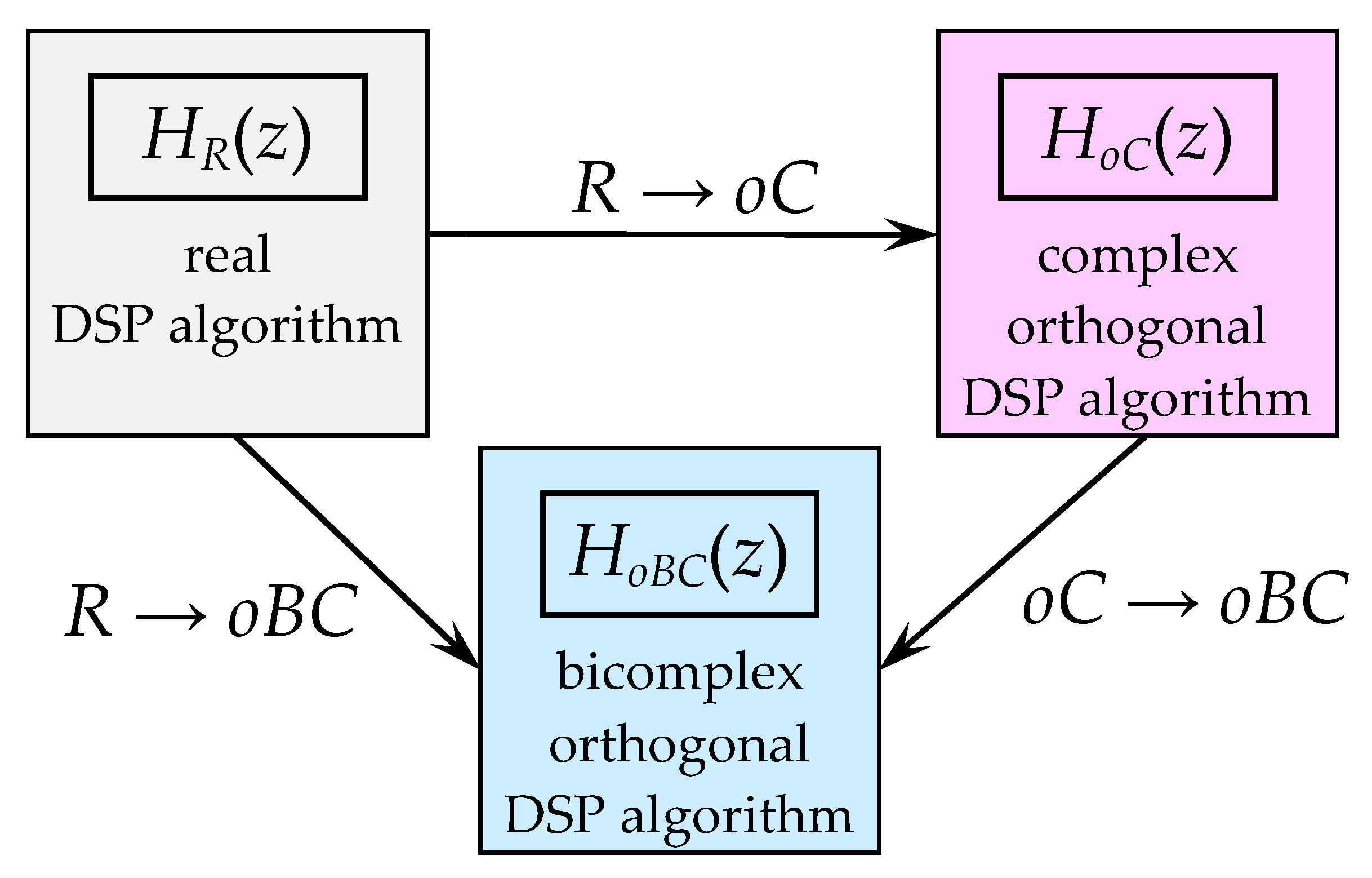
The transformation that leads to bicomplex orthogonal digital algorithms can be obtained starting from either a real (R → oBC) or a complex algorithm (oC → oBC), as shown in Figure 1. The transfer functions H_R(z), H_oC(z), and H_oBC(z) denote real, complex, and orthogonal in regard to the vector unit i, and bicomplex orthogonal algorithms in the complex z-domain, respectively.

Along with (27), the other two transformations in trigonometric form to design an orthogonal bicomplex DSP algorithm (Figure 1) when θ₂ = 45° are as follows:

$$R\to oC:\hspace{1em}{z}^{-1}\to i{z}^{-1};\hspace{1em}{i}^2=-1,$$

(28)

$$oC\to oBC:\hspace{1em}{z}^{-1}\to z^{-1}\frac{\sqrt{2}}{2}\left(1+j\right);\hspace{1em}{j}^2=-1.$$

(29)

After applying the orthogonal complex transformation R → oC (28), the poles of the real transfer function H_R(z) rotate clockwise and counterclockwise at an angle of θ₁ = 90°, and double in number. The rotation of the single pole of a bilinear real digital algorithm, resulting in a pair of complex–conjugate poles on the imaginary axis of the corresponding orthogonal complex algorithm, is shown in Figure 2.

The complex–bicomplex orthogonal substitution oC → oBC (29) will again double the poles compared to the real bilinear transfer function, so that those of the bicomplex orthogonal bilinear transfer function will be four in total. As a type, these four poles will be two complex–conjugate pairs (Figure 2). Here, the rotation is as follows: each pole of the orthogonal complex DSP algorithm rotates 45° once clockwise and once counterclockwise. Thus, each pole is multiplied into two new ones belonging to the orthogonal bicomplex DSP algorithm.

The steps to be followed to design an orthogonal bicomplex digital algorithm—represented by its transfer function H_oBC(z)—when starting from a real algorithm H_R(z), which is first transformed into an orthogonal complex H_oC(z) algorithm, are shown in Figure 3.

The alternative approach directly accomplishes the transformation of an orthogonal real DSP algorithm into an orthogonal bicomplex one. The sequence of the necessary transformations of this alternative approach is shown in Figure 4. The designations of the transfer functions in Figure 3 and Figure 4 are unified.

The design approaches presented in Figure 3 and Figure 4 show that an N-order bicomplex orthogonal transfer function H_oBC(z) can be represented by its scalar part H_oS(z) and vector part H_oV(z), both of which are complex coefficient functions of the 2N-order. In accordance with bicomplex number arithmetic, the scalar and vector parts can be derived via the bicomplex orthogonal transfer function and its vector conjugate, as follows:

$$\begin{array}{c}{H}_{oS}(z)=\frac{1}{2}\left[H_{oBC}(z)+H_{oBC}^{+}(z)\right];\\ H_{oV}(z)=\frac{1}{2i}\left[H_{oBC}(z)-H_{oBC}^{+}(z)\right].\end{array}$$

(30)

Additionally, H_oBC(z) can be also represented by the four real coefficient transfer functions of the 4N-order H_o1(z), H_o2(z), H_o3(z), and H_o4(z), which comprise the scalar H_oS(z) and vector H_oV(z) parts, but on the other hand can also be determined via them, as follows:

$$\begin{array}{l}\begin{array}{l}{H}_{o1}(z)=\frac{1}{2}\left[H_{oS}(z)+H_{oS}^{*}(z)\right];\hfill \\ H_{o2}(z)=\frac{1}{2j}\left[H_{oS}(z)-H_{oS}^{*}(z)\right];\hfill \end{array}\\ \begin{array}{l}{H}_{o3}(z)=\frac{1}{2}\left[H_{oV}(z)+H_{oV}^{*}(z)\right];\hfill \\ H_{o4}(z)=\frac{1}{2j}\left[H_{oV}(z)-H_{oV}^{*}(z)\right].\hfill \end{array}\end{array}$$

(31)

Either of the two approaches of the proposed new method represented in Figure 3 and Figure 4 will lead to the same final result—the design of a bicomplex orthogonal DSP algorithm. However, the approach that involves first deriving a complex orthogonal digital algorithm starting from a real coefficient algorithm and then designing the corresponding bicomplex orthogonal DSP algorithm enables issues such as the sensitivity and canonicity of the three structures—real, complex, and bicomplex—to be compared and contrasted.

5. Bilinear Orthogonal Bicomplex DSP Algorithm Derivation—A Numerical Example

The effect of the proposed new method will be demonstrated for a particular digital algorithm, represented in the z-domain by the most simple bilinear recursive real transfer function possible:

$$H_R(z)=c\frac{1}{1-a{z}^{-1}},$$

(32)

where the coefficient c = 1 − a provides unity DC gain.

When applying the orthogonal bicomplex method shown in Figure 3 to the real bilinear transfer function H_R(z) (32), the following transfer functions describing orthogonal complex and orthogonal bicomplex digital algorithms will be obtained:

$$H_R\left(z\right)\stackrel{z^{-1}=i{z}^{-1}}{\to }{H}_{oC}\left(z\right)=c\frac{1}{1-ia{z}^{-1}}=H_{oR1}(z)+i{H}_{oR2}(z),$$

(33)

where:

$$H_{oR1}(z)=\frac{1-a^2}{1+a^2{z}^{-2}};\hspace{1em}\hspace{1em}\hspace{1em}{H}_{oR2}(z)=\frac{\left(1-a^2\right)z^{-1}}{1+a^2{z}^{-2}}.$$

(34)

Applied on the orthogonal complex H_oC(z), the transformation (29) will produce the orthogonal bicomplex transfer function H_oBC(z):

$$H_{oBC}\left(z\right)=c\frac{1}{1-\left(\sqrt{2}/2\right)i\left(1+j\right)a{z}^{-1}}=H_{oS}(z)+i{H}_{oV}(z),$$

(35)

where the scalar and vector parts H_oS(z) and H_oV(z), respectively, are:

$$H_{oS}\left(z\right)=\frac{1-a}{1+j{a}^2{z}^{-2}};\hspace{1em}\hspace{1em}\hspace{1em}{H}_{oV}\left(z\right)=\frac{\frac{\sqrt{2}}{2}a\left(1-a\right)\left(1+j\right)z^{-1}}{1+j{a}^2{z}^{-2}}.$$

(36)

Subsequently, the real coefficient transfer functions H_o1(z), H_o2(z), H_o3(z), and H_o4(z), are determined as follows, respectively:

$$\begin{array}{l}{H}_{o1}(z)=\frac{1-a^4}{1+a^4{z}^{-4}};\\ H_{o2}(z)=\frac{\left(1-a^4\right)z^{-2}}{1+a^4{z}^{-4}};\\ H_{o3}(z)=\sqrt{2}\left(1-a^2\right)\frac{z^{-1}\left(1+a^2{z}^{-2}\right)}{1+a^4{z}^{-4}};\\ H_{o4}(z)=\sqrt{2}\left(1-a^2\right)\frac{z^{-1}\left(1-a^2{z}^{-2}\right)}{1+a^4{z}^{-4}}.\end{array}$$

(37)

The alternative approach of Figure 4 will also derive the orthogonal bicomplex transfer function H_oBC(z):

$$H_R\left(z\right)\stackrel{z^{-1}=\frac{\sqrt{2}}{2}i\left(1+j\right)z^{-1}}{\to }{H}_{oBC}\left(z\right)=H_{oC1}(z)+j{H}_{oC2}(z),$$

(38)

where:

$$H_{oC1}\left(z\right)=c\frac{1-i\frac{\sqrt{2}}{2}a{z}^{-1}}{1-i\sqrt{2}a{z}^{-1}-a^2{z}^{-2}};\hspace{1em}\hspace{1em}\hspace{1em}\hspace{1em}{H}_{oC2}\left(z\right)=c\frac{i\frac{\sqrt{2}}{2}a{z}^{-1}}{1-i\sqrt{2}a{z}^{-1}-a^2{z}^{-2}}.$$

(39)

The functions in (39) have complex coefficients with respect to the vector unit i, and as complex functions can be represented by their real and imaginary parts, which are the four transfer functions with real coefficients in (37). The real coefficient transfer functions delivered in this section—namely, (32), (34), and (37)—will be analysed in the frequency domain.

Having two inputs and two outputs, the orthogonal complex scheme in Figure 5a is able to realize four real biquadrate transfer functions at its different outputs. These are identical within each pair, and equal to H_oR1(z) and H_oR2(z) (34), respectively:

$$\begin{array}{l}{H}_{RR}(z)=H_{II}(z)=H_{oR1}(z),\\ H_{RI}(z)=-H_{IR}(z)=H_{oR2}(z).\end{array}$$

(40)

Likewise, the orthogonal bicomplex realization (Figure 5b), having 4 inputs and 4 outputs, will have 16 fourth-order real coefficient transfer functions altogether, separated into 4 groups. The four functions in each group are identical, with a plus or a minus sign, and are also equal to the transfer functions shown in (37):

$$\begin{array}{c}{H}_{11}\left(z\right)=\hspace{1em}{H}_{22}\left(z\right)=\hspace{1em}{H}_{33}\left(z\right)=H_{44}\left(z\right)=H_{o1}\left(z\right);\\ -H_{12}\left(z\right)=\hspace{1em}{H}_{21}\left(z\right)=-H_{34}\left(z\right)=H_{43}\left(z\right)=H_{o2}\left(z\right);\\ -H_{13}\left(z\right)=-H_{24}\left(z\right)=\hspace{1em}{H}_{31}\left(z\right)=H_{42}\left(z\right)=H_{o3}\left(z\right);\\ H_{14}\left(z\right)=-H_{23}\left(z\right)=\hspace{1em}{H}_{32}\left(z\right)=H_{41}\left(z\right)=H_{o4}\left(z\right).\end{array}$$

(41)

When H_R(z) (32) is low-pass (LP), H_oR1(z) and H_oR2(z) (34) will both be of band-pass (BP) type, while the four bicomplex orthogonal transfer functions—H_o1(z), H_o2(z), H_o3(z), and H_o4(z) (37)—are also of BP type, but with two passbands each. A high-pass (HP) H_R (z) will produce both BP and band-stop (BS) transfer functions (34), and in the bicomplex case the transfer functions (37) will again be multiband, having two passbands for the BP type and two stopbands for the BS type.

Narrowband frequency-selective digital signal processing is the most likely to be used in practice. When the numerical value of the coefficient a of the real transfer function H_R(z) (32) is 0.99, the real bilinear digital algorithm becomes narrowband and LP; its magnitude and phase responses, together with those of the corresponding orthogonal complex H_oR1(z) (34) and the bicomplex H_o1(z) (37) constituents, are shown in Figure 6.

The magnitude responses are unity for DC, achieved by scaling the examined real coefficient transfer functions. The scaling factor for H_R(z) is c = 1−a, for H_oR1(z) it is c_R1 = 1−a², and for H_o1(z) it is c_o1 = 1−a⁴. Since the experimental results for the other complex and bicomplex orthogonal transfer functions—H_oR2(z), H_o2(z), H_o3(z), and H_o4(z)—are similar, they are not represented in this work.

6. Conclusions

In this paper, a method of designing orthogonal bicomplex DSP algorithms is outlined. The proposed technique is based on the idea behind the pole rotation complex orthogonal transformation in the z-domain, and converts real or complex algorithms into bicomplex orthogonal ones. The new orthogonal method is universal, since it is not affected by either the order or the type of the real algorithm used, and it guarantees the synthesis of digital structures with a canonical number of elements. The method is related to the orthogonal multiple access (OMA) modulation techniques based on filtering (UFMS, f-OFDM), and a comparison to these methods can highlight its advantages.

Due to the wide implementation of narrowband orthogonal frequency-selective DSP algorithms, this type of LP transfer function is used as a numerical example to demonstrate the operation of the method. The resulting bicomplex orthogonal BP/BS functions doubled the number of the passbands/stopbands compared to the complex functions, inheriting the real and complex transfer functions’ narrowband properties.

The method proposed is also appropriate for the derivation of second- or higher order digital algorithms, thus providing different bicomplex digital structures and realizations, such as cascade, parallel, etc., of any order. In addition to being simple and canonical, these structures offer parallelism and unification, which will result in a lower equipment cost, reduced complexity, and higher energy efficiency, and could be appropriate for the enhancement of the implementation of intelligent algorithms in next-generation RANs, enabling a diverse range of novel usage scenarios, addressing ultralow latency requirements, and allowing intelligent performance of diverse functions, such as load balancing, radio resource management, interference detection and mitigation, etc.

Different aspects of bicomplex orthogonality in the design of bicomplex DSP algorithms, as outlined in the present work, have not yet been exhaustively investigated, and more research remains to be done. Along with this, a subject of future research might be the efficiency levels of the different types of bicomplex orthogonality for processing waveforms of arbitrary complexity, which can be represented as real, complex, or bicomplex signals. Effective bicomplex DSP algorithms can be a powerful tool for the advanced processing units in modern telecommunications.