Douglas–Rachford Splitting Method with Linearization for the Split Feasibility Problem

Abstract

The aim of this article is to introduce the Douglas–Rachford splitting method with linearization to solve the split feasibility problem (SFP). Our proposed method includes two existing methods in work of Tang et al. and Wang as special cases. The ranges of the parameters in work of Tang et al. are extended from (0,1) to (0,2). Under standard conditions, we prove the weak convergence of proposed algorithms. We also provide two numerical experiments to illustrate the effectiveness of the proposed algorithm by comparing the algorithms in work of Tang et al. and Wang.

1. Introduction

In this article, we consider the split feasibility problem (SFP) in the form

$$\mathrm{find}{x}^{*}\in C\mathrm{and}A{x}^{*}\in Q,$$

(1)

where C and Q are the nonempty closed convex subsets of the real Hilbert spaces ${\mathcal{H}}_1$ and ${\mathcal{H}}_2$, respectively, and $A:{\mathcal{H}}_1\to {\mathcal{H}}_2$ is a bounded linear operator. The SFP was introduced by Censor and Elfving [1] for inverse problems which arise from phase retrievals and medical image reconstruction [2] and were later generalized to the multiple-sets split feasibility problem [3].

Throughout this article, we assume that the SFP (1) is consistent, i.e., its solution set, denoted by

$$\Gamma =\{x|x\in C\mathrm{and}Ax\in Q\},$$

is nonempty.

By transforming the SFP as an equivalent constrained optimization problem, Byrne [2,4] firstly introduced the well-known CQ algorithms, which have received a great deal of attention from many authors, who improved it in various ways; see, e.g., [5,6,7,8,9,10,11,12].

To solve the SFP (1), Wang [13] introduced the following gradient method which was called Polyak’s gradient method:

$$x^{k+1}=x^k-{\tau }_k\left[(x^k-P_C{x}^k)+A^{*}(I-P_Q)A{x}^k\right],$$

(2)

where

$${\tau }_k={\rho }_k\frac{\parallel x^k-P_C{x}^k{\parallel }^2+||(I-P_Q)A{x}^k{||}^2}{2\parallel (x^k-P_C{x}^k)+A^{*}(I-P_Q)A{x}^k{\parallel }^2},$$

and ${\rho }_k\in (0,2).$ In fact, (2) is a special case of the so-called simple projection method in [14]. The authors [15] proposed an iterative method for solving the multiple-sets split feasibility problem with splitting self-adaptive stepsizes, which reduces to the following scheme when applied to the SFP (1):

$$x^{k+1}=x^k-\left[{\mu }_k(x^k-P_C{x}^k)+{\nu }_k{A}^{*}(I-P_Q)A{x}^k\right],$$

(3)

where ${\mu }_k\in (0,1)$ and

$${\nu }_k={\sigma }_k\frac{\parallel (I-P_Q)A{x}^k{\parallel }^2}{\parallel A^{*}(I-P_Q)A{x}^k{\parallel }^2},$$

and ${\sigma }_k\in (0,1).$ Note that the difference of the schemes (2) and (3) is the choices of the stepsizes.

The Douglas–Rachford splitting method introduced in [16] is a popular method to solve structured optimization problems. Let g and h be proper lower semicontinuous convex functions from a Hilbert space $\mathcal{H}$ to $(-\infty ,+\infty )$. Consider the structured optimization problem:

$$\underset{x\in \mathcal{H}}{min}g(x)+h(x).$$

Given the initial guess $x^0$, the Douglas–Rachford splitting method generates the iterative sequence via the following scheme:

$$\left\{\begin{array}{c}{y}^{k+1}=\underset{x\in \mathcal{H}}{argmin}\left\{g(y)+\frac{1}{2{\lambda }_k}||y-x^k{||}^2\right\},\hfill \\ z^{k+1}=\underset{z\in \mathcal{H}}{argmin}\left\{h(z)+\frac{1}{2{\lambda }_k}||z-(2y^{k+1}-x^k){||}^2\right\},\hfill \\ x^{k+1}=x^k+{\alpha }_k(z^{k+1}-y^{k+1}),\hfill \end{array}\right.$$

(4)

where ${\{{\alpha }_k\}}_{k\in \mathbb{N}}\subset (0,2)$ is a parameter sequence and ${\{{\lambda }_k\}}_{k\in \mathbb{N}}\subset (0,\infty )$ is the proximal parameter sequence of the regularization terms. Note that the scheme (4) with ${\{{\alpha }_k\}}_{k\in \mathbb{N}}\subset (0,+\infty )$ was called the general splitting method in [17] and becomes the Peaceman–Rachford splitting method when ${\{{\alpha }_k\}}_{k\in \mathbb{N}}\subset [2,+\infty ).$

It is easy to see that the split feasibility problem (1) also equals the following unconstrained minimization problem:

$$\underset{x\in {\mathcal{H}}_1}{min}\left\{{\iota }_C(x)+f(x)\right\},$$

(5)

where $f(x)=\frac{1}{2}{\parallel (I-P_Q)Ax\parallel }^2$ and ${\iota }_C(x)$ is the indicator function of the set C; that is, ${\iota }_C(x)=0$ if $x\in C$, otherwise ${\iota }_C(x)=+\infty$. Recall that the gradient of $f(x)$ is $\nabla f(x)=A^{*}(I-P_Q)Ax$. Letting $g=f$ and $h={\iota }_C$ in (4) and using the linearization technique, the authors [18] recently introduced the following general splitting methods with linearization for the SFP (1):

$$\left\{\begin{array}{c}{y}^{k+1}:=x^k-{\lambda }_k\nabla f(x^k),\hfill \\ z^{k+1}:=P_C(2y^{k+1}-x^k),\hfill \\ x^{k+1}:=x^k+{\alpha }_k(z^{k+1}-y^{k+1}),\hfill \end{array}\right.$$

(6)

where ${\{{\alpha }_k\}}_{k\in \mathbb{N}}$ is a sequence of positive numbers and

$${\lambda }_k:=\left\{\begin{array}{cc}\gamma \frac{{\displaystyle f(x^k)}}{{\displaystyle \parallel \nabla f(x^k){\parallel }^2}},\hfill & \mathrm{if}\nabla f(x^k)\ne 0,\hfill \\ 0,\hfill & \mathrm{otherwise},\hfill \end{array}\right.$$

and $\gamma \in (0,2).$ The weak convergence of the algorithm (6) was established under the standard conditions, and the algorithm (6) has good numerical performance comparing the algorithm (2) and Algorithm 3.1 in [10].

In this article, we present an iterative scheme by letting $g={\iota }_C$ and $h=f$ in (4) and using the linearization technique. The convergence of the corresponding scheme is analyzed.

The rest of the paper is constructed as follows. In Section 2, we recall some definitions and known results for further analysis. In Section 3, we present the Douglas–Rachford splitting method with linearization and its relaxed version. In Section 4, we show the weak convergence of the proposed algorithm, which converges weakly to a solution of the SFP. In Section 5, we give two numerical experiments to show the behavior of the algorithm. Finally, some concluding remarks are given in Section 6.

2. Preliminaries

Let $\mathcal{H}$ be a Hilbert space and K be a nonempty closed convex subset of $\mathcal{H}$. We use the notation:

• ⇀ for weak convergence and → for strong convergence;
• ${\omega }_w(x^k)=\{x:\exists x^{k_l}\rightharpoonup x\}$ denotes the weak $\omega$-limit set of ${\{x^k\}}_{k\in \mathbb{N}}$.

The following identity will be used for the main results (see [19], Corollary 2.15):

$${\parallel \alpha x+(1-\alpha )y\parallel }^2={\alpha \parallel x\parallel }^2+{(1-\alpha )\parallel y\parallel }^2-\alpha (1-\alpha ){\parallel x-y\parallel }^2$$

(7)

for all $\alpha \in \mathbb{R}$ and $(x,y)\in \mathcal{H}\times \mathcal{H}$.

Definition 1

([19], Definition 6.38). Let K be a nonempty convex subset of $\mathcal{H}$ and let $x\in \mathcal{H}$. The normal cone to K at x is

$$N_K(x)=\left\{\begin{array}{cc}\left\{u\in \mathcal{H}|sup\langle K-x,u\rangle \le 0\right\},\hfill & \mathrm{if}x\in K;\hfill \\ \varnothing ,\hfill & \mathrm{otherwise}.\hfill \end{array}\right.$$

For a point x, the the classical metric projection of x onto K, denoted by $P_K(x)$, is defined by

$$P_K(x):=argmin\{\parallel x-y\parallel :\forall y\in K\}.$$

Lemma 1

([19], Proposition 4.4). For any $x,y\in \mathcal{H}$ and $z\in K$, the following hold:

(i) 

$\parallel P_K(x)-P_K{(y)\parallel }^2\le \langle P_K(x)-P_K(y),x-y\rangle ;$

(ii) 

$\parallel P_K{(x)-z\parallel }^2\le {\parallel x-z\parallel }^2-{\parallel P_K(x)-x\parallel }^2$;

(iii) 

$\langle (I-P_K)x-(I-P_K)y,x-y\rangle \ge {\parallel (I-P_K)x-(I-P_K)y\parallel }^2.$

It follows from Lemma 1 (iii) that

$$\langle x-P_K(x),x-z\rangle \ge {\parallel x-P_K(x)\parallel }^2,\forall x\in \mathcal{H},\forall z\in K.$$

(8)

Recall that a mapping $T:\mathcal{H}\to \mathcal{H}$ is called to be nonexpansive if

$$\parallel Tx-Ty\parallel \le \parallel x-y\parallel ,\forall x,y\in \mathcal{H}.$$

Lemma 1 (i) implies that $P_K$ is firmly nonexpansive and consequently nonexpansive.

The next lemma shows that the nonexpansive mappings are demiclosed at 0.

Lemma 2

([19], Theorem 4.27). Let K be a nonempty closed convex subset of $\mathcal{H}$ and $T:K\to \mathcal{H}$ be a nonexpansive mapping. Let ${\{x^k\}}_{k\in \mathbb{N}}$ be a sequence in K and $x\in \mathcal{H}$ such that $x^k\rightharpoonup x$ and $T{x}^k-x^k\to 0$ as $k\to +\infty$. Then $x\in \mathrm{Fix}(T)$.

Lemma 3

([19], Lemma 2.47). Let K be a nonempty closed convex subset of $\mathcal{H}$ and ${\{x^k\}}_{k\in \mathbb{N}}$ be a sequence in $\mathcal{H}$ such that the following two conditions hold:

(i) 

For all $x\in K$, ${lim}_{n\to \infty }\parallel x^k-x\parallel$ exists;

(ii) 

Every sequential weak cluster point of ${\{x^k\}}_{k\in \mathbb{N}}$ is in K.

Then the sequence ${\{x^k\}}_{k\in \mathbb{N}}$ converges weakly to a point in K.

3. Douglas–Rachford Splitting Method with Linearization

In this section, we introduce Douglas–Rachford splitting method with linearization and its relaxed variant.

Using symmetry, we can set $g={\iota }_C$ and $h=f$ in (4). Now, we present a direct adaptation of the Douglas–Rachford splitting method (4), which can solve the equivalent problem (5) of the SFP (1). (see Algorithm 1)

Algorithm 1 Douglas–Rachford splitting method.

Step 0. Input $k:=0$, $x^0\in {\mathcal{H}}_1$. Step 1. Generate $x^{k+1}$ by $$\left\{\begin{array}{c}{y}^{k+1}:=P_C(x^k),\hfill \\ z^{k+1}:=\underset{z\in {\mathcal{H}}_1}{argmin}\left\{f(z)+\frac{1}{2{\lambda }_k}{\parallel z-(2y^{k+1}-x^k)\parallel }^2\right\},\hfill \\ x^{k+1}:=x^k+{\alpha }_k\left(z^{k+1}-y^{k+1}\right),\hfill \end{array}\right.$$ (9) where ${\{{\alpha }_k\}}_{k\in \mathbb{N}}$ and ${\{{\lambda }_k\}}_{k\in \mathbb{N}}$ are sequences of positive numbers. Step 2. If a termination criterion is not met, then set $k:=k+1$ and go to Step 1.

By the first-order optimality condition of the second formula of (9) in Algorithm 1,

$$\begin{array}{c}0=\nabla f(z^{k+1})+\frac{1}{{\lambda }_k}\left[z^{k+1}-(2y^{k+1}-x^k)\right]\hfill \\ =A^{*}(I-P_Q)A{z}^{k+1}+\frac{1}{{\lambda }_k}\left[z^{k+1}-(2y^{k+1}-x^k)\right].\hfill \end{array}$$

To calculate $z^{k+1}$, we need to get ${(I+{\lambda }_k{A}^{*}(I-P_Q)A)}^{-1}$, which is very difficult. In order to overcome this difficulty, we linearize $f(z)$ at $x^k$. Then, the second formula of (9) becomes

$$\begin{array}{ll}{z}^{k+1}:& =\underset{z\in {\mathcal{H}}_1}{argmin}\left\{f(x^k)+\langle \nabla f(x^k),z-x^k\rangle +\frac{1}{2{\lambda }_k}{\parallel z-(2y^{k+1}-x^k)\parallel }^2\right\}\\ & =\underset{z\in {\mathcal{H}}_1}{argmin}\left\{\langle \nabla f(x^k),z-x^k\rangle +\frac{1}{2{\lambda }_k}{\parallel z-(2y^{k+1}-x^k)\parallel }^2\right\}.\end{array}$$

Its first-order optimality condition is

$$\nabla f(x^k)+\frac{1}{{\lambda }_k}[z^{k+1}-(2y^{k+1}-x^k)]=0.$$

Then we have

$$z^{k+1}=2y^{k+1}-x^k-{\lambda }_k\nabla f(x^k).$$

Thus, we get the following linearized Douglas–Rachford splitting method:

$$\left\{\begin{array}{c}{y}^{k+1}:=P_C(x^k),\hfill \\ z^{k+1}:=2y^{k+1}-x^k-{\lambda }_k\nabla f(x^k),\hfill \\ x^{k+1}:=x^k+{\alpha }_k\left(z^{k+1}-y^{k+1}\right).\hfill \end{array}\right.$$

After a simple calculation, we get

$$x^{k+1}:=x^k+{\alpha }_k\left[P_C(x^k)-x^k-{\lambda }_k\nabla f(x^k)\right].$$

In what follows, we present the Douglas–Rachford splitting method with linearization. (see Algorithm 2)

Algorithm 2 Douglas–Rachford splitting method with linearization.

Step 0. Input $k:=0$, $x^0\in {\mathcal{H}}_1$. Step 1. Given $x^k$, generate $x^{k+1}$ by $$x^{k+1}:=x^k-{\alpha }_k\left[(x^k-P_C(x^k))+{\lambda }_k{A}^{*}(I-P_Q)A{x}^k\right],$$ where ${\{{\alpha }_k\}}_{k\in \mathbb{N}}$ and ${\{{\lambda }_k\}}_{k\in \mathbb{N}}$ are two sequences of positive numbers. Step 2. If $\nabla f(x^k)=0$ and $x^{k+1}=x^k$, then terminate. Otherwise, set $k:=k+1$ and go to Step 1.

Remark 1.

Algorithm 2 is a general scheme with two parameters sequences ${\{{\alpha }_k\}}_{k\in \mathbb{N}}$ and ${\{{\lambda }_k\}}_{k\in \mathbb{N}}$, which includes the algorithms (2) and (3) as special cases. Indeed,

(i) 

Let ${\alpha }_k={\tau }_k$ and ${\lambda }_k\equiv 1$, $\forall k\in \mathbb{N};$ then, Algorithm 2 becomes the algorithm (2);

(ii) 

Let ${\alpha }_k={\mu }_k$ and ${\lambda }_k=\frac{{\nu }_k}{{\mu }_k},$ $\forall k\in \mathbb{N};$ then, Algorithm 2 becomes the algorithm (3).

In the following, we extend the ranges of the parameter sequences ${\{{\mu }_k\}}_{k\in \mathbb{N}}$ and ${\{{\sigma }_k\}}_{k\in \mathbb{N}}$ in the algorithm (3). To this end, let ${\alpha }_k={\beta }_k\theta$ and

$${\lambda }_k=\frac{(1-{\beta }_k)\rho }{{\alpha }_k}{\eta }_k,$$

where ${\beta }_k\in (0,1),$ $\theta \in (0,2)$, $\rho \in (0,2)$ and

$${\eta }_k=\frac{\parallel (I-P_Q)A{x}^k{\parallel }^2}{\parallel A^{*}(I-P_Q)A{x}^k{\parallel }^2}.$$

Then, Algorithm 2 becomes

$$x^{k+1}=x^k-{\beta }_k\theta (x^k-P_C(x^k))-(1-{\beta }_k)\rho {\eta }_k{A}^{*}(I-P_Q)A{x}^k.$$

(10)

Note that ${\beta }_k\theta \in (0,2)$ and $(1-{\beta }_k)\rho \in (0,2)$. Comparing (3) and (10), the ranges of the parameter sequences ${\{{\mu }_k\}}_{k\in \mathbb{N}}$ and ${\{{\sigma }_k\}}_{k\in \mathbb{N}}$ in the algorithm (3) are extended from (0,1) to (0,2). It is worth noting that ${\{{\mu }_k\}}_{k\in \mathbb{N}}$ and ${\{{\sigma }_k\}}_{k\in \mathbb{N}}$ cannot both be in (1,2). In fact, one is in (0,2), while the other is in (0,1). Due to ${\alpha }_k\in (0,2)$, Algorithm 2 is the Douglas–Rachford splitting method with linearization.

We give two choices of ${\beta }_k$, as follows:

• Constant choice: ${\beta }_k:=\beta \in (0,1)$ for all $k\in \mathbb{N}$;
• Adaptive choice: Let $\underline{\beta },\overline{\beta }\in (0,1)$,

  $${\beta }_k^{*}=\frac{1}{2}+\frac{\theta (2-\theta ){∥x^k-P_C(x^k)∥}^2-\rho (2-\rho ){\eta }_k{∥(I-P_Q)A{x}^k∥}^2}{2{∥\theta (x^k-P_C(x^k))-\rho {\eta }_k{A}^{*}(I-P_Q)A{x}^k∥}^2},$$

  (11)

  and ${\beta }_k=max\{\underline{\beta },min\{{\beta }_k^{*},\overline{\beta }\}\}$.

Note that the upper and lower bounds are imposed in the adaptive choice of ${\beta }_k$ to guarantee ${\beta }_k\in (0,1)$. Therefore, it is not fully adaptive.

Now, the following lemma shows the validity of the stopping criterion through Step 2 of the Douglas–Rachford splitting method with linearization.

Lemma 4.

If $\nabla f(x^k)=0$ and $x^{k+1}=x^k$ for some k, then $x^k$ generated by Algorithm 2 is a solution of the SFP (1).

Proof. 

Using $\nabla f(x^k)=0$ and $x^{k+1}=x^k$, we get $x^k=P_C(x^k)$, which implies $x^k\in C.$ Thus, $0\in N_C(x^k).$ We deduce that $x^k$ is a solution of the SFP (1) because of the first-order optimality condition $0\in N_C(x)+\nabla f(x)$ of problem (5). □

In Algorithm 2, we generally assume that the projections $P_C$ and $P_Q$ are easy to calculate. However, projection is sometimes impossible or difficult to calculate. In order to solve this problem, we consider a general situation of C and Q in SFP (1). $C=\{x\in {\mathcal{H}}_1:c(x)\le 0\}$ and $Q=\{y\in {\mathcal{H}}_2:q(y)\le 0\}$ are level sets, where $c:{\mathcal{H}}_1\to \mathbb{R}$ and $q:{\mathcal{H}}_2\to \mathbb{R}$ are convex functions. We assume that $\partial c$ and $\partial q$ are bounded operators and define the sets $C_k$ and $Q_k$ as follows:

$$C_k=\left\{x\in {\mathcal{H}}_1:c(x^k)+\langle {\xi }^k,x-x^k\rangle \le 0\right\},$$

where ${\xi }^k\in \partial c(x^k)$, and

$$Q_k=\left\{y\in {\mathcal{H}}_2:q(A{x}^k)+\langle {\eta }^k,y-A{x}^k\rangle \le 0\right\},$$

where ${\eta }^k\in \partial q(A{x}^k)$.

Next, we define $f_k(x):=\frac{1}{2}{\parallel (I-P_{Q_k})Ax\parallel }^2$ and introduce the relaxed Douglas–Rachford splitting method with linearization. (see Algorithm 3)

Algorithm 3 Relaxed Douglas–Rachford splitting method with linearization.

Step 0. Input $k:=0$, $x^0\in {\mathcal{H}}_1$. Step 1. Given $x^k$, generate $x^{k+1}$ by $$x^{k+1}:=x^k-{\alpha }_k\left[(x^k-P_{C_k}(x^k))+{\lambda }_k{A}^{*}(I-P_{Q_k})A{x}^k\right],$$ (12) where ${\{{\alpha }_k\}}_{k\in \mathbb{N}}$ and ${\{{\lambda }_k\}}_{k\in \mathbb{N}}$ are two sequences of positive numbers. Step 2. If $\nabla f_k(x^k)=0$ and $x^{k+1}=x^k$, then terminate. Otherwise, set $k:=k+1$ and go to Step 1.

4. Convergence Analysis

In this section, we prove the weak convergence of Algorithm 2 under the standard conditions.

Firstly, we present two lemmas which are key for the convergence of Algorithm 2.

Lemma 5.

Let ${\{x^k\}}_{k\in \mathbb{N}}$ be the sequence generated by Algorithm 2 from any initial point $x^0\in {\mathcal{H}}_1$ and $x^{*}\in \Gamma$. Let ${\beta }_k\equiv \beta \in (0,1),$ $\forall k\in \mathbb{N}.$ Then it holds

$$\begin{array}{ll}{∥x^{k+1}-x^{*}∥}^2\le & {∥x^k-x^{*}∥}^2-\beta \theta (2-\theta ){∥x^k-P_C(x^k)∥}^2\\ & -(1-\beta )\rho (2-\rho ){\eta }_k{∥(I-P_Q)A{x}^k∥}^2\\ & -\beta (1-\beta ){∥\theta (x^k-P_C(x^k))-\rho {\eta }_k{A}^{*}(I-P_Q)A{x}^k∥}^2.\end{array}$$

(13)

Proof. 

By (10) and (7), we have

$$\begin{array}{c} {∥x^{k+1}-x^{*}∥}^2\hfill \\ ={\parallel {\beta }_k[x^k-\theta (x^k-P_C(x^k))-x^{*}]+(1-{\beta }_k)[x^k-\rho {\eta }_k{A}^{*}(I-P_Q)A{x}^k-x^{*}]\parallel }^2\hfill \\ =\beta {∥x^k-x^{*}-\theta (x^k-P_C(x^k))∥}^2\hfill \\ +(1-\beta ){∥x^k-x^{*}-\rho {\eta }_k{A}^{*}(I-P_Q)A{x}^k∥}^2\hfill \\ -\beta (1-\beta ){∥\theta (x^k-P_C(x^k))-\rho {\eta }_k{A}^{*}(I-P_Q)A{x}^k∥}^2.\hfill \end{array}$$

(14)

Using (8), we get

$$〈x^k-x^{*},x^k-P_C(x^k)〉\ge {∥x^k-P_C(x^k)∥}^2,$$

(15)

and

$$〈x^k-x^{*},A^{*}(I-P_Q)A{x}^k〉=〈A{x}^k-A{x}^{*},(I-P_Q)A{x}^k〉\ge {∥(I-P_Q)A{x}^k∥}^2.$$

(16)

By (15), we obtain

$$\begin{array}{c} {∥x^k-x^{*}-\theta (x^k-P_C(x^k))∥}^2\hfill \\ ={∥x^k-x^{*}∥}^2+{\theta }^2{∥x^k-P_C(x^k)∥}^2-2\theta 〈x^k-x^{*},x^k-P_C(x^k)〉\hfill \\ \le {∥x^k-x^{*}∥}^2-\theta (2-\theta ){∥x^k-P_C(x^k)∥}^2.\hfill \end{array}$$

(17)

From (16) and the definition of ${\eta }_k$, it follows

$$\begin{array}{c} {∥x^k-x^{*}-\rho {\eta }_k{A}^{*}(I-P_Q)A{x}^k∥}^2\hfill \\ ={∥x^k-x^{*}∥}^2+{\rho }^2{\eta }_k^2{∥A^{*}(I-P_Q)A{x}^k∥}^2-2\rho {\eta }_k〈x^k-x^{*},A^{*}(I-P_Q)A{x}^k〉\hfill \\ \le {∥x^k-x^{*}∥}^2+{\rho }^2{\eta }_k^2{∥A^{*}(I-P_Q)A{x}^k∥}^2-2\rho {\eta }_k{∥(I-P_Q)A{x}^k∥}^2\hfill \\ ={∥x^k-x^{*}∥}^2-\rho (2-\rho ){\eta }_k{∥(I-P_Q)A{x}^k∥}^2.\hfill \end{array}$$

(18)

Combining (14), (17) and (18), we deduce (13). The proof is completed. □

Remark 2.

The inequality (13) with the ranges of the parameters $\beta ,\theta ,\rho$ shows the monotonically decreasing property of the sequence $\{\parallel x^k-x^{*}{||\}}_{k\in \mathbb{N}}$. It is not the same as the inequality in [15], and the latter reduces to the following form for the SFP (1):

$$\begin{gathered} {∥x^{k+1}-x^{*}∥}^2\le {∥x^k-x^{*}∥}^2-2{\mu }_k(1-{\mu }_k){∥x^k-P_C(x^k)∥}^2 \\ -2{\sigma }_k(1-{\sigma }_k){\eta }_k{∥(I-P_Q)A{x}^k∥}^2. \end{gathered}$$

It is difficult to compare them and show which is better in theory. The numerical experiments in Section 5 illustrate that the optimal choices of the parameters of ${\{{\mu }_k\}}_{k\in \mathbb{N}}$ and ${\{{\sigma }_k\}}_{k\in \mathbb{N}}$ is that one is in (0,2) while the others are in (0,1).

Lemma 6.

Let ${\{x^k\}}_{k\in \mathbb{N}}$ be the sequence generated by Algorithm 2 from any initial point $x^0\in {\mathcal{H}}_1$, $x^{*}\in \Gamma$. Let ${\beta }_k$ is given adaptively.

(i) 

If ${\beta }_k^{*}\in [\underline{\beta },\overline{\beta }]$, it holds

$$\begin{array}{c} {∥x^{k+1}-x^{*}∥}^2\hfill \\ \le {∥x^k-x^{*}∥}^2-\frac{1}{2}\theta (2-\theta ){∥x^k-P_C(x^k)∥}^2\hfill \\ -\frac{1}{2}\rho (2-\rho ){\eta }_k{∥(I-P_Q)A{x}^k∥}^2\hfill \\ -\frac{1}{4}{∥\theta (x^k-P_C(x^k))-\rho {\eta }_k{A}^{*}(I-P_Q)A{x}^k∥}^2\hfill \\ -\frac{{\left[\theta (2-\theta ){∥x^k-P_C(x^k)∥}^2-\rho (2-\rho ){\eta }_k{∥(I-P_Q)A{x}^k∥}^2\right]}^2}{4{∥\theta (x^k-P_C(x^k))-\rho {\eta }_k{A}^{*}(I-P_Q)A{x}^k∥}^2};\hfill \end{array}$$

(19)

(ii) 

If ${\beta }_k^{*}\notin [\underline{\beta },\overline{\beta }]$, it holds

$$\begin{array}{c}{∥x^{k+1}-x^{*}∥}^2\le {∥x^k-x^{*}∥}^2-\underline{\beta }\theta (2-\theta ){∥x^k-P_C(x^k)∥}^2\hfill \\ -(1-\overline{\beta })\rho (2-\rho ){\eta }_k{∥(I-P_Q)A{x}^k∥}^2\hfill \\ -(\underline{\beta }-{\overline{\beta }}^2){∥\theta (x^k-P_C(x^k))-\rho {\eta }_k{A}^{*}(I-P_Q)A{x}^k∥}^2.\hfill \end{array}$$

(20)

Proof. 

(i) In this case, ${\beta }_k={\beta }_k^{*}$. Similar to Lemma 5, we have

$$\begin{array}{c}{∥x^{k+1}-x^{*}∥}^2\le {∥x^k-x^{*}∥}^2-{\beta }_k\theta (2-\theta ){∥x^k-P_C(x^k)∥}^2\hfill \\ -(1-{\beta }_k)\rho (2-\rho ){\eta }_k{∥(I-P_Q)A{x}^k∥}^2\hfill \\ -{\beta }_k(1-{\beta }_k){∥\theta (x^k-P_C(x^k))-\rho {\eta }_k{A}^{*}(I-P_Q)A{x}^k∥}^2.\hfill \end{array}$$

(21)

Let

$$\begin{array}{c}{d}_k=\theta (2-\theta ){∥x^k-P_C(x^k)∥}^2,\hfill \\ e_k=\rho (2-\rho ){\eta }_k{∥(I-P_Q)A{x}^k∥}^2,\hfill \\ m_k={\parallel \theta (x^k-P_C(x^k))-\rho {\eta }_k{A}^{*}(I-P_Q)A{x}^k\parallel }^2.\hfill \end{array}$$

The inequality (21) becomes

$$\parallel x^{k+1}-x^{*}{\parallel }^2\le {\parallel x^k-x^{*}\parallel }^2-{\beta }_k{d}_k-(1-{\beta }_k)e_k-{\beta }_k(1-{\beta }_k)m_k.$$

(22)

After simple calculations, we get

$$\begin{array}{c} -{\beta }_k{d}_k-(1-{\beta }_k)e_k-{\beta }_k(1-{\beta }_k)m_k\hfill \\ =m_k{\beta }_k^2-(d_k-e_k+m_k){\beta }_k-e_k\hfill \\ =m_k{({\beta }_k-\frac{d_k-e_k+m_k}{2m_k})}^2-m_k{(\frac{1}{2}+\frac{d_k-e_k}{2m_k})}^2-e_k\hfill \\ =-\frac{1}{2}{d}_k-\frac{1}{2}{e}_k-\frac{m_k}{4}-\frac{{(d_k-e_k)}^2}{4m_k},\hfill \end{array}$$

(23)

where the last equality holds due to (11). Combining (22) and (23), we get (19);

(ii) In this case, ${\beta }_k=\underline{\beta }$ or ${\beta }_k=\overline{\beta }$. By Lemma 5, it is easy to obtain (20). □

Theorem 1.

Let ${\{x^k\}}_{k\in \mathbb{N}}$ be generated by Algorithm 2; then, ${\{x^k\}}_{k\in \mathbb{N}}$ converges weakly to a solution of the SFP (1).

Proof. 

By (13), (19) and (20), we have

$$\parallel x^{k+1}-x^{*}\parallel \le \parallel x^k-x^{*}\parallel ,$$

which implies that ${\{x^k\}}_{k\in \mathbb{N}}$ is bounded and ${lim}_{k\to \infty }\parallel x^k-x^{*}\parallel$ exists. From the definition of ${\eta }_k$, it follows

$${\eta }_k=\frac{\parallel (I-P_Q)A{x}^k{\parallel }^2}{\parallel A^{*}(I-P_Q)A{x}^k{\parallel }^2}\ge \frac{\parallel A{x}^k-P_Q(A{x}^k){\parallel }^2}{{\parallel A\parallel }^2{\parallel A{x}^k-P_Q(A{x}^k)\parallel }^2}=\frac{1}{{\parallel A\parallel }^2}.$$

(24)

Combining (13), (19), (20) and (24), we deduce

$$\underset{k\to \infty }{lim}\parallel P_C(x^k)-x^k\parallel =0,$$

(25)

and

$$\underset{k\to \infty }{lim}\parallel (I-P_Q)A{x}^k\parallel =0.$$

(26)

To use Lemma 3, we need to show ${\omega }_w(x^k)\subseteq \Gamma$. To this end, take arbitrarily $\widehat{x}\in {\omega }_w(x^k)$ and let $x^{k_l}\rightharpoonup \widehat{x}$ where ${\{x^{k_l}\}}_{l\in \mathbb{N}}$ is a subsequence of ${\{x^k\}}_{k\in \mathbb{N}}$. From Lemma 2 and (25), we get $\widehat{x}\in C$. Combining (26) and the weak lower semicontinuity of f, we obtain

$$0\le f(\widehat{x})\le \underset{l\to \infty }{lim\; inf}f(x^{k_l})=\underset{k\to \infty }{lim}f(x^k)=0.$$

Hence, $f(\widehat{x})=\frac{1}{2}\parallel (I-P_Q)A\widehat{x}\parallel =0$, i.e., $A\widehat{x}\in Q$. Thus, we have ${\omega }_w(x^k)\subseteq \Gamma$. By Lemma 3, we deduce that ${\{x^k\}}_{k\in \mathbb{N}}$ converges weakly to a point in $\Gamma$. The proof is completed. □

Combining Theorem 1 and [18] (Theorem 3.2), it is easy to verify the convergence of Algorithm 3.

Theorem 2.

Let ${\{x^k\}}_{k\in \mathbb{N}}$ be generated by Algorithm 3; then, ${\{x^k\}}_{k\in \mathbb{N}}$ converges weakly to a solution of the SFP (1).

5. Numerical Results

In this section, we show the behavior of Algorithm 2 by comparing it with the algorithms (3) and (2) through two numerical examples.

For convenience, we denote the vector with all elements 0 by $e_0$ and the vector with all elements 1 by $e_1$ in what follows. In the next two numerical examples, we take the objective function value $p(x)=\frac{1}{2}\parallel x-P_C{(x)\parallel }^2+\frac{1}{2}{\parallel Ax-P_Q(Ax)\parallel }^2\le ϵ$ as the stopping criterion.

Example 1

([6]). Consider the SFP, where $A={(a_{ij})}_{m\times n}\in {\mathbb{R}}^{m\times n}$ ($m=200,n=500$) and $a_{ij}\in (0,1)$ generated randomly and

$$\begin{array}{c}C=\{x\in {\mathbb{R}}^n:\parallel x-d\parallel \le r\},\hfill \\ Q=\{y\in {\mathbb{R}}^m:L\le y\le U\},\hfill \end{array}$$

where d is the center of the ball C, $e_0\le d\le e_1$, $r\in (10,20)$ is the radius, d and r are both generated randomly. L and U are the boundary of the box Q and are also generated randomly, satisfying $10e_1\le L\le 20e_1$ and $20e_1\le U\le 30e_1$, respectively.

In the numerical experiment, we take the objective function value $p(x^k)\le ϵ={10}^{-5}$ as the stopping criterion.

In Figure 1, the initial point $x^0\in (0,100e_1)$ is randomly chosen. For comparing Algorithm 2 with the algorithms (2) and (3), we take $\theta =1.59$, $\rho =1.86$ and ${\beta }_k\equiv \beta =0.37$ in Algorithm 2, ${\rho }_k=1.99$ in the algorithm (2) and ${\mu }_k=0.72$ and ${\nu }_k=0.88$ in the algorithm (3).

In

Table 1. Comparison of Algorithm 2, algorithms (2) and (3) under different initial points.

Cases	Algorithm 2		algorithm (2)		algorithm (3)
	Iter.	CPU Time	Iter.	CPU Time	Iter.	CPU Time
Case 1	18	0.0313	155	0.0313	38	0.0469
Case 2	22	0.0469	372	0.0781	37	0.0469
Case 3	16	0.0313	256	0.0469	35	0.0313

, we show the iteration steps and CPU time of Algorithm 2, algorithm (2) and algorithm (3) for 3 initial points. For case 1, $x^0=(100,\cdots ,100)$; for case 2, $x^0$ = (100, −100, ⋯, 100, −100); and for case 3, $x^0\in (-100e_1,100e_1)$.

As shown in Figure 1 and the iteration steps in Table 1, Algorithm 2 behaves better than the algorithms (2) and (3).

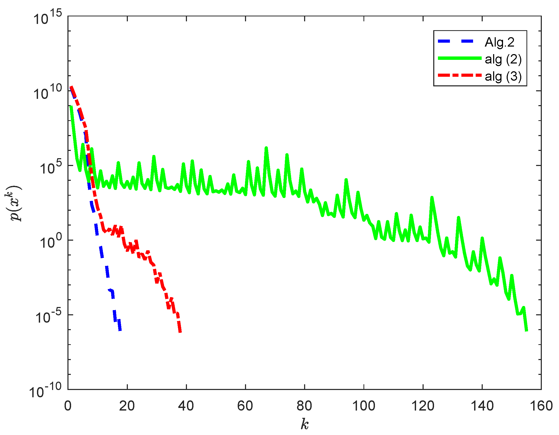
Example 2.

Suppose that ${\mathcal{H}}_1={\mathcal{H}}_2=L^2([0,1])$ with norm $\parallel x\parallel ={\left({\int }_0^1{|x(t)|}^{2}dt\right)}^{\frac{1}{2}}$ and inner product

$$\langle x,y\rangle ={\int }_0^{1}x(t)y(t)dt.$$

Let

$$C:=\{x\in {\mathcal{H}}_1:\langle a,x\rangle =b\},$$

where $a=sin(5t^3)$ and $b=0$. In this case, we have

$$P_C(x)=x+\frac{b-\langle a,x\rangle }{{\parallel a\parallel }^2}a.$$

Additionally, let

$$Q:=\{x\in {\mathcal{H}}_2:\langle c,x\rangle \le d\},$$

where $c=sin(t/4)$ and $d=1/5$; then, we obtain

$$P_Q(x)=\left\{\begin{array}{cc}x\hfill & \mathrm{if}\langle c,x\rangle \le d\hfill \\ x+\frac{d-\langle c,x\rangle }{{\parallel c\parallel }^2}c\hfill & \mathrm{if}\langle c,x\rangle >d.\hfill \end{array}\right.$$

Consider the matrix

$$A=\frac{1}{200}{\left(\begin{array}{cccccc}0& 0& 0& \cdots & 0& 0\\ 1& 1& 0& \cdots & 0& 0\\ 1& 2& 1& \cdots & 0& 0\\ ⋮& ⋮& ⋮& \ddots & ⋮& ⋮\\ 1& 2& 2& \cdots & 1& 0\\ 1& 2& 2& \cdots & 2& 1\end{array}\right)}_{101\times 101}$$

resulting from a discretization of the operator question of the first kind

$$y(t)=(Ax)(t):={\int }_0^{t}x(s)ds,s,t\in [0,1];x,y:[0,1]⟶[0,1].$$

In the numerical experiment, the initial function is $x^0(t)=10sin(t^2+2t)$. We take $p(x^k)\le ϵ={10}^{-10}$ as the stopping criterion.

For comparing Algorithm 2 with the algorithms (2) and (3), we take $\theta =1.99$, $\rho =1.99$ and ${\beta }_k\equiv \beta =0.41$ in Algorithm 2, ${\rho }_k=1.89$ in the algorithm (2) and ${\mu }_k=0.5$ and ${\nu }_k=0.99$ in the algorithm (3). From Figure 2, we can see that the performance of Algorithm 2 is better than the algorithms (2) and (3).

6. Some Concluding Remarks

In this article, we introduce the Douglas–Rachford splitting method with linearization for the split feasibility problem, which is a general method and includes the methods in [13,15] as special cases. The weak convergence of the proposed method is established under the standard conditions. Numerical experiments illustrate the effectiveness of our methods.

The methods proposed in this article can be generalized to solve the multiple-sets split feasibility problem. It is interesting to investigate the other possible choices of the parameters ${\{{\alpha }_k\}}_{k\in \mathbb{N}}$ and ${\{{\lambda }_k\}}_{k\in \mathbb{N}}$.

Recently, some authors have applied self-adaptive step sizes to split generalized equilibrium and fixed point problems [20] and pseudo-monotone equilibrium problems [21]. The numerical examples illustrate that the step sizes have excellent behaviour. Applying the self-adaptive step size to the split feasibility problem is worth investigating.