
Stable Calculation of Discrete Hahn Functions


Philips Research, 5656 AE Eindhoven, The Netherlands
Symmetry 2022, 14(3), 437; https://doi.org/10.3390/sym14030437
Submission received: 3 February 2022
/
Revised: 16 February 2022
/
Accepted: 21 February 2022
/
Published: 23 February 2022
(This article belongs to the Special Issue Symmetries of Difference Equations, Special Functions and Orthogonal Polynomials)
Abstract
:Generating discrete orthogonal polynomials from the recurrence or difference equation is error-prone, as it is sensitive to error propagation and dependent on highly accurate initial values. Strategies to handle this, involving control over the deviation of norm and orthogonality, have already been developed for the discrete Chebyshev and Krawtchouk functions, i.e., the orthonormal basis in derived from the polynomials. Since these functions are limiting cases of the discrete Hahn functions, it suggests that the strategy could also be successful there. We outline the algorithmic strategies including the specific method of generating the initial values, and show that the orthonormal basis can indeed be generated for large supports and polynomial degrees with controlled numerical error. Special attention is devoted to symmetries, as the symmetric windows are most commonly used in signal processing, allowing for simplification of the algorithm due to this prior knowledge, and leading to savings in the required computational power.
1. Introduction
There is a long history in fundamental research on orthogonal polynomials. In the current age where information is transmitted and stored in predominantly digital ways, discrete orthogonal polynomials are finding their way into applications such as signal processing systems. The classical discrete orthogonal polynomials encompass the well-known discrete Chebyshev, Krawtchouk and Hahn polynomials [1].
For signal processing applications, unitary transformations derived from the polynomial systems are of interest. The recurrence relation and difference equation associated with these polynomials carry over to the basis functions defining these unitary transforms. It has been noted however, that deployment of these properties in iterative computation schemes (e.g., for generating the basis functions) gives rise to numerical issues. This not always an issue, as many applications operate with transformations having small support and/or low polynomial degree, e.g., in image processing, typically small patches of images or video signals are analyzed or coded. The question remains whether there is a general and elegant way in line with the theory of normed spaces such that these numerical issues are mitigated for the general case.
Several strategies have been proposed to deal with these issues [2,3,4,5], typically geared to a specific polynomial system, or targeting specific applications. Recently, an approach based on truncating the tails of the functions has been proposed for the discrete Chebyshev and Krawtchouk functions [6,7]. It is in these tails that numerical problems manifest themselves. The truncation, i.e., the operational definition of tail, is controlled by the norm of the basis functions and thus fits in well with the basic notions in these systems. It is this research trail that we will follow.
Since the discrete Chebyshev and Krawtchouk polynomials are limiting cases of discrete Hahn polynomials, we expect a similar approach to work here as well. The present paper confirms this, provided that adequate measures are taken to mitigate numerical issues with the initial samples in these recursive schemes. We will highlight the common aspects and differences in the developed tail-cutting approaches, with special attention to polynomials associated with symmetric weight functions, since on the one hand, the prior knowledge of symmetry typically allows for alternative solutions and decreased computational complexity, while on the other hand, they are presumed dominant in many application domains.
The outline of this paper is as follows. We first introduce the discrete Hahn polynomials and their notation in line with literature. Then we turn to the discrete Hahn functions, and review properties underlying our algorithmic strategy and the chosen experimental settings for validation (Section 3). Next, we consider the strategies, while also relating them to the limiting cases and with special attention to the symmetric weight functions (Section 4). In Section 5, we validate the performance. We close with our conclusions.
2. Discrete Hahn Polynomials
We consider a discrete finite interval represented by variable x with . For the notation of the orthogonal polynomials, we dominantly follow [8].
2.1. Weight Function
The weight function underlying the discrete Hahn polynomials is given by
with or and with the Pochhammer function denoting the rising factorial [8]. The shape of weight function is defined by these two parameters that allow to steer the location and width of the peak. Examples of the influence of the parameters on the weight function are shown in Figure 1. If , the maximum of the weight function occurs for ; if the window is symmetric. Particularly, the freedom in the window’s effective width at each N is an asset provided by the Hahn polynomials compared to the discrete Chebyshev and Krawtchouk cases.
For later use, we note that the ratio between two consecutive weight samples is a ratio of two second-degree polynomials:
The limiting cases are characterized by the fact that this fraction reduces to a constant (discrete Chebyshev) or a ratio of first-order polynomials (Krawtchouk).
2.2. Discrete Hahn Polynomials
In line with [8], the discrete Hahn polynomials are denoted as , or in shorthand notation, . The latter is dominantly used in this paper as it is mostly unnecessary to explicitly state the dependence on N, and . It also allows us, when relevant, to consider as representing the limiting cases: the discrete Chebyshev or Krawtchouk polynomials, polynomials not belonging to the allowed range of . Expressions of the polynomials in terms of Rodrigues’ Formula and generalized hypergeometric function can be found in [8]. We note that swapping the roles of corresponds to mirroring the support and an amplitude correction
2.3. Normalization Constant
The normalization constant of the discrete Hahn polynomial is given by [8]
Note: if then and .
The normalized window is defined as
2.4. Recurrence Relation
2.5. Difference Equation
3. Discrete Hahn Functions
The discrete Hahn functions are defined as
We refer to these as functions and not as normalized polynomials for obvious reasons. We therefore also speak about the order of the Hahn functions as opposed to the degree of the Hahn polynomials. In order to be consistent, we use the same terminology and distinctions for Krawtchouk and for discrete Chebyshev, even though, due to the fact of a constant weight function, the discrete Chebyshev functions are in fact polynomials.
Putting all samples of the discrete Hahn functions into an matrix yields an orthonormal transformation matrix. An arbitrary sequence of numbers (e.g., a segment from a discrete-time signal) can thus be mapped onto this polynomial domain. Depending on the application, certain operations can be applied in this domain such as de-trending (attenuating the lower-order components), de-noising (attenuating or removing higher-order components), or searching for particular patterns (like in watermarking).
The discrete Hahn functions inherit the symmetry property (3) from the polynomials in the following form
i.e., swapping the roles of the parameters is equivalent to reversal of the x-axis.
3.1. Recurrence Relation
The recurrence relation for the discrete Hahn functions becomes
with
3.2. Difference Equation
3.3. Energy: Center and Spread
It is well-known that using the recurrence and difference equation to create the associated transformation matrix creates numerical issues, e.g., [2,3,4,5]. These issues occur at positions in the plane where consecutive values of are small and thus the precision of the numerical representation has a relatively large effect. To obtain insight into where these spots occur, we consider the center and spread of the discrete Hahn functions.
For the center and spread (or width) of the energy of a discrete function , we use the standard definitions:
The center of a function f on a discrete domain is defined as
The effective width of a function f on a discrete domain is defined as
We are interested in the center and spread of the discrete Hahn function and denote its center and spread as and , respectively.
By virtue of the recurrence relations and explicit knowledge of its coefficients, explicit expressions for the center and effective width of each Hahn function are available [9]. For the center we have
It is easy to show that if . In other cases, the center is a monotonically increasing or decreasing function of n, but unlike the Krawtchouk case, is not linearly dependent on n. For the effective width we have
These features of the Hahn functions can be displayed in the plane, as shown in Figure 2, where for each function order n the central lobe is visualized by the boundaries . This gives a contour in the plane within which the energy of the functions are concentrated. We observe that depending on whether or <N, the spread is higher or lower for higher orders.
We consider the center and width of the zeroth-order function in more detail. The center is given by
Values of x close to this will presumably be good starting points for recursion. This is considered in more detail at the end of the next section.
To illustrate the spread variation, we consider symmetric weight functions: . For convenience, we introduce
and show the effect of on the normalized spread in Figure 3. For each N, it consist of two sigmoidal components, associated with positive and negative values of . For positive , the normalized spread is between , corresponding to flat window (discrete Chebyshev), and the width of a Krawtchouk zeroth-order function: . Using negative , the width can be further reduced by a factor to . These graphs will be used to guide the selection of settings for the validation trials.
In contrast to the Krawtchouk case where energy concentration could be easily determined in the polynomial domain [7] due to the specific form of , this is not case for the discrete Hahn functions.
4. Strategies
In this section, we consider the strategies to generate the discrete functions for all values of x and for orders from 0 to some user-defined maximum order . The setting for this maximum depends on the application and is related with the amount of detail that needs to be maintained in the mapping. The discussed strategies relate to the various functions (discrete Chebyshev, Krawtchouk, discrete Hahn) and the presence of symmetries useful to deploy in the algorithms. This includes the strategy for accurate initialization. The essential differences between this procedure and previous approaches [2,3,4,5] are
- Repeated careful initialization at each new order;
- The use of a norm-based stop criterion.
The processing further distinguishes itself by a balancing principle. Both for the computation of the initial values and for the order in which samples are calculated, a control mechanism is in place based on prior knowledge of the end result of the recursive operations. In the first case, this is such that the normalized weight function is strictly less than 1 at each x, in the second case it is the location of the center of the function .
4.1. Symmetries
The discrete Hahn functions are fundamentally asymmetric; only for a symmetry or antisymmetry occurs with respect to the center of the interval . Additionally, the discrete Chebyshev and Krawtchouk with display this symmetry and the strategies developed before are included in the discussion. Krawtchouk functions display further symmetries along the diagonal and antidiagonal for all values of p, meaning there are fundamental similarities of functions in the original and transform domain. This, however, has no direct counterpart in the discrete Hahn functions.
4.2. Scheme Based on the Recurrence Relation
For discrete Chebyshev functions , the zeroth-order function is trivial as it is a constant. Furthermore, the weight function is symmetric, inducing symmetric and antisymmetric patterns in the even and odd functions, respectively. Although the discrete Chebyshev functions are usually defined on an interval , in the following we assume they are defined like the Krawtchouk and Hahn polynomials on an interval . If N is odd, it means only half of the samples need to be calculated; via mirroring plus sign reversal for odd n, all other values are available. This means samples need to be calculated. For even N, one might think one needs to calculate samples, but at the antisymmetry for odd n implies that values are 0. The total is therefore slightly less than that.
For the discrete Chebyshev functions, the recursive relation (RR) is executed starting at . While recursing over n, the norm can be tracked over the already calculated samples at each x, separately, i.e.,:
If this norm is sufficiently close to 1, all function values at this x for higher orders are set to zero. This prevents numerical issues that would otherwise occur for large values of n and large (and small) values of x. The concept is sketched in Figure 4.
We presume that this strategy will also work in practice for the discrete Hahn functions if the weight function is sufficiently flat. However, since it is not a general approach and since it is not a priori clear exactly what sufficiently flat implies in terms of allowed parameters, we will not consider this further.
4.3. Strategies Based on Symmetry
A separate strategy is in place for symmetric weight functions. It thus applies to the discrete Chebyshev, Krawtchouk with and discrete Hahn functions with .
Let us assume that we can calculate highly accurate values for and where . For these two values of x, the recursive relation can be applied without problems as they are located in the central lobe of the energy. These two x-values can subsequently be used as starting points for the deployment of the difference equation (DE). Like in the discrete Chebyshev case, we can track the energy associated with samples generated so far, but do this now along the x variable, i.e.,
The DE calculation is then truncated whenever the norm is sufficiently close to 1.
The strategy is sketched in Figure 5. In the Krawtchouk case, the number of computations can be reduced even further as a consequence of symmetries over diagonals.
4.4. Strategies Based on Tracking Point of Gravity
The general procedure is an adaptation of the symmetric case. In the symmetric case, the DE is executed starting at the center of the interval . For the general situation, we must realize that this is not a good choice a priori; instead, we expect x values close to the center to provide highly accurate start values for the DE. Therefore, the recurrence relation is not taken along the center of the interval but along the center of energy, as sketched in Figure 6.
The procedure for generating the discrete Hahn functions is explained in more detail in the flowchart of Figure 7. Input are the transformation parameters: and the control parameter . The control parameter indicates the allowed deviation from unit norm of each generate discrete Hahn function. Furthermore, a maximum value for the order can be supplied: .
Given these input parameters, the algorithm determines and stores the coefficients of the recurrence relation and difference equation. Once this is done, a loop over the order n is executed, starting with and running until . Within this loop, first the center of energy is considered; in fact it has already been calculated as it equals one of the recurrence relation parameters, see (19). This value is translated into two integer values of x closest to it: and . If , the recurrence relation is used to generate at these values from the lower-order samples. If , they are generated by the initialization procedure discussed in Section 4.5. From these initial values, the associated norm is determined, thereby starting the norm tracking. Additionally, the actual center of energy, i.e., that associated with the samples generated so far, is determined. Depending on whether the actual center is lower or higher than the real center , the range of x-values at this particular n is extended in the upper of lower boundary of the existing range by the difference equation (DE). After having generated this new sample , the norm is updated and compared with the stop criterion. If it is lower, we proceed to generate a new sample at this order by returning to the block deciding whether to extend at the lower or higher range. If the criterion is met, all samples outside the already generated range of x are set to 0 (zero-padding). The order is increased by one, and if less than the maximum order, the process starts with the steps to calculate the samples at this updated order n.
The flowchart is simple and straightforward for the discrete Hahn functions. In case of the Krawtchouk functions, we can deploy the symmetries over the diagonal and antidiagonal, as illustrated in Figure 6, to make the scheme more efficient. This requires some extra checks to see if, when having crossed a diagonal, values can be picked up from mirroring. This may or may not be the case, as for previous orders an independent decision has been taken to terminate the calculations. The extra logic is not shown in the flowchart as it pertains only to the Krawtchouk case, not to the general discrete Hahn functions.
4.5. Initialization at
It is paramount to have initial values with high accuracy, and to calculate these such that no numerical problems occur even for extreme parameters. For instance, calculations deploying standard routines for the function fail rather quickly.
The next procedure addresses this issue. The algorithm as discussed above requires at and . We have and the normalized window (5) can be expressed as a product series of N terms by
There are other ways to express in a product series, but this one has properties that make it attractive. We also note that as a consequence of the normalization (5).
Let us assume that (implying ), where we note this can always be attained by swapping roles of and , see (3). This implies that we have more terms (i.e., ) in the right-hand product series than in the first one. We note that each term in the product series running from to N is less than 1. The terms in the left-hand product series are a decreasing sequence as function of k.
It is important to note that taking the product formation in the order of the index results in very high values as an intermediate result, potentially resulting in overflows. Arbitrary ordering has the risk of over- or under-flows. To mitigate that issue, we use a controlled product execution method based on the fact that the final result (the normalized window in the center) is always less that 1. We store all N ratios from the expression in a list ordered according to index k. All ratios larger than one are at the top of the list; below that, only ratios less than 1 appear. Let us call the intermediate product P. The control strategy is the following. If P is larger than 1, we update the result by multiplying it with the first entry from the list and remove that ratio from the list. Otherwise, we multiply with the highest ratio (last in the list) and remove the last entry. This is done until the list of ratios is empty. The effect is that the intermediate product will fluctuate around 1 until all ratios larger than or equal to 1 have been removed from the list. From then on, the intermediate product P decreases monotonically. Having , we take the square root to obtain and use (2) to obtain .
The initial points for the symmetric case () are the center points. If N is even, then the maximum of occurs at , and from (5), is given by
i.e., a product series of length consisting of squared ratios. If N is even, and we define , then the maximum of occurs at M and and is given by
where in the general case we have N product terms, here we have less. The same procedure as for the general case can be applied to avoid numerical overflows. It is obvious that for the symmetric case it is convenient to calculate directly as a product series rather than .
We note that the sketched procedure for determining the initial values is by no means the only possibility. As an example, accurate approximations exist for the ratio of -functions that may be deployed instead, in case of specific parameters. The merit of the proposed procedure is that it provides a generic approach and leads to a simple algorithmic solution.
5. Results
5.1. Parameters in the Experiments
For validation of the proposed procedure, we use two sizes for N: 200 and 2000. Based on the range of shapes of the symmetric windows as shown in Figure 3, we opted for three positive and three negative values of covering the full range, meaning one representative for the middle of the sigmoidal function, and two values close to the saturation levels. For symmetric windows and the proposed interval sizes, this gives the settings for as displayed in columns 2 and 4 of Table 1.
For asymmetric weight functions, we controlled the position of to cover the full range. We choose five settings of where the center increases approximately by 1/(10N), starting at 1/(20N); for we used a setting already used for the symmetric weight functions and corresponding to the center of the sigmoidal functions, as shown in Figure 3.
We choose a large range of allowed deviations , where each parameter setting has its specific value for visualization purposes.
5.2. Symmetric Weight Functions
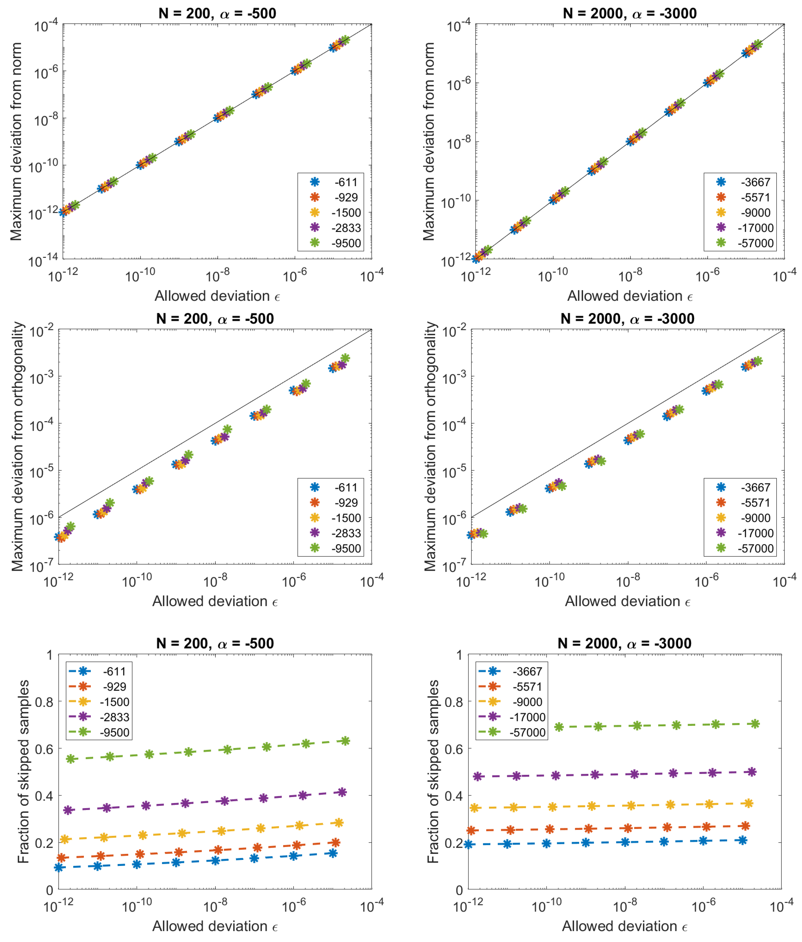
In Figure 8, the results of the validation are shown for discrete Hahn functions associated with symmetric weight functions. For those orders where truncation occurs, the maximum deviation from norm is always smaller than the specified deviation. For those orders where no zero-padding occurs, the deviation of unit norm is induced by the machine accuracy and can result in larger deviations than specified. This is visible for and , where for the measured deviation is above the black line. The orthogonality, although not explicitly controlled, is below . The amount of zero-padding is only slightly affected by the specified accuracy: at , 20% of the samples were set to 0.
5.3. General Weight Functions
In Figure 9 and Figure 10, the results of the validation are shown for asymmetric weight functions. Again, for those orders where truncation occurs, the maximum deviation from norm is always smaller than the specified deviation. The orthogonality is below . The amount of zero-padding is only slightly affected by the specified accuracy. The amount of skewness, however, has a large influence: with at 5 % of the full interval, more than half of the data are set to 0 in case of negative values of .
6. Discussion
The validation results show that the proposed algorithm mitigates the issues of error propagation effectively with a user-controlled deviation from norm and also a bound on the achieved deviation from orthogonality. Still, to make the algorithm student-proof, it may be good to add some control over the input parameters, where a check is made for if the parameter combination is still meaningful. This can be achieved by calculating and and providing warnings at high eccentricities and inappropriate , i.e., those close to limit of the range.
The case of discrete Hahn functions based on symmetric windows are presumably the most widely used ones in practice, e.g., in image processing, the orientation left or right would not logically warrant different behavior. In applications, the basis functions can be calculated and stored upfront. The calculation of the basis functions associated with symmetric weight functions is computationally less demanding, but more importantly, so is the transformation itself. The input signal can be split upfront into a symmetric and antisymmetric function. Then, the transformation breaks down into two separate processes where only half of the computations are needed. The additional overhead is the (low-cost) decomposition into symmetric and antisymmetric input signal, and the reshuffling of coefficients at the end.
7. Conclusions
An algorithm for generating discrete Hahn functions based on recurrence relations and difference equations has been described. The algorithm mitigates the issue of error propagation by a combination of controlling where to use the recurrence relation, how to choose the direction in which the difference equation is applied, and where to apply zero-padding. The control mechanism is based on tracking the norm and on explicit prior knowledge of the center of energy. We have shown that the strategy is effective.
Special attention has been paid to the relations with the limiting cases of discrete Chebyshev and Krawtchouk functions, and to simplifications occurring for the discrete Hahn systems associated with a symmetric weight function.
The sketched method is general by nature; the flowchart shows that the premises are that the parameters in the recurrence relation and difference equation can be computed, and that highly accurate initial values at the first pattern () can be created.
Funding
This research received no external funding.
Institutional Review Board Statement
Not applicable.
Informed Consent Statement
Not applicable.
Data Availability Statement
Not applicable.
Acknowledgments
The author thanks R. Rietman and R. van Dinther for suggestions on an early version of the paper. Thanks to the reviewers for corrections and helpful suggestions.
Conflicts of Interest
The author declares no conflict of interest.
References
- Hahn, W. Über Orthogonalpolynome, die q-Differenzengleichungen genügen. Math. Nachrichten 1949, 2, 4–34. [Google Scholar] [CrossRef]
- Zhang, G.; Luo, Z.; Fu, B.; Li, B.; Liao, J.; Fan, X.; Xi, Z. A symmetry and bi-recursive algorithm of accurately computing Krawtchouk moments. Pattern Recognit. Lett. 2010, 31, 548–554. [Google Scholar] [CrossRef]
- Abdulhussain, S.H.; Ramli, A.R.; Al-Haddad, S.A.R.; Mahmmod, B.M.; Jassim, W.A. Fast recursive computation of Krawtchouk polynomials. J. Math. Imaging Vis. 2018, 60, 285–303. [Google Scholar] [CrossRef]
- Mahmmod, B.M.; Abdul-Hadi, A.M.; Abdulhussain, S.H.; Hussien, A. On computational aspects of Krawtchouk polynomials for high orders. J. Imaging 2020, 6, 81. [Google Scholar] [CrossRef]
- Daoui, A.; Karmouni, H.; Sayyouri, M.; Hassan, Q. Fast and stable computation of higher-order Hahn polynomials and Hahn moment invariants for signal and image analysis. Multimed. Tools Appl. 2021, 80, 32947–32973. [Google Scholar] [CrossRef]
- den Brinker, A.C. Controlled accuracy for discrete Chebyshev polynomials. In Proceedings of the 2020 28th European Signal Processing Conference (EUSIPCO), Amsterdam, The Netherlands, 18–21 January 2021; pp. 2279–2283. [Google Scholar]
- den Brinker, A.C. Stable calculation of Krawtchouk functions from triplet relations. Mathematics 2021, 9, 1972. [Google Scholar] [CrossRef]
- Koornwinder, T.H.; Wong, R.S.C.; Koekoek, R.; Swarttouw, R.F. Hahn Class: Definitions. In NIST Handbook of Mathematical Functions; Olver, F., Lozier, D., Boisvert, R., Clark, C., Eds.; Cambridge University Press: New York, NY, USA, 2010. [Google Scholar]
- den Brinker, A.C.; Belt, H.J.W. Optimal free parameters in orthonormal approximations. IEEE Trans. Signal Process. 1998, 46, 2081–2087. [Google Scholar] [CrossRef] [Green Version]
Figure 1.
Examples of discrete Hahn weight functions. (Left): , (middle): and (right): . In all cases , and as indicated in the legend.
Figure 1.
Examples of discrete Hahn weight functions. (Left): , (middle): and (right): . In all cases , and as indicated in the legend.

Figure 2.
Examples of energy concentration of the Hahn functions for , where the colored lines indicate energy center ± the standard deviation for each order n. (Left): as indicated in legend, and (right): various combinations of as indicated.
Figure 2.
Examples of energy concentration of the Hahn functions for , where the colored lines indicate energy center ± the standard deviation for each order n. (Left): as indicated in legend, and (right): various combinations of as indicated.

Figure 3.
Examples of normalized energy spread for symmetric as function of .

Figure 4.
Algorithmic strategy for the calculation of the discrete Chebyshev functions. The process is initiated by calculation of the zeroth-degree function. The termination of executing the recurrence relation depends on the attained norm (in the n direction) and differs per x. The striped area indicates the part that need not be calculated but can be obtained from symmetry.

Figure 5.
Algorithmic strategy for the calculation of the functions in case of symmetric weight functions. (Left): discrete Hahn and discrete Chebyshev functions; (right): Krawtchouk functions. The striped area indicates the part that need not be calculated but can be obtained from symmetry. The recurrence relation runs over the central values of x, and the difference equation is used for the other values, starting from the center of the interval. Termination of the execution of the difference equation depends on the attained norm and is evaluated at each n independently.

Figure 6.
Schematic representation of the algorithm. (Left): discrete Hahn functions, (right): Krawtchouk functions. The striped area indicates parts that need not be calculated but can be obtained from symmetry. The recurrence relation is used for samples x closest to the center of energy.
Figure 6.
Schematic representation of the algorithm. (Left): discrete Hahn functions, (right): Krawtchouk functions. The striped area indicates parts that need not be calculated but can be obtained from symmetry. The recurrence relation is used for samples x closest to the center of energy.

Figure 7.
Flowchart for the computation of discrete Hahn functions. The variables and E denote the center of energy and energy of the nth-order discrete Hahn function based on the samples calculated so far.
Figure 7.
Flowchart for the computation of discrete Hahn functions. The variables and E denote the center of energy and energy of the nth-order discrete Hahn function based on the samples calculated so far.

Figure 8.
Results for symmetric weight functions. From top to bottom: maximum deviation from norm, maximum deviation from orthogonality and fraction of samples created by zero-padded. Left column: , right column: . The legend gives .
Figure 8.
Results for symmetric weight functions. From top to bottom: maximum deviation from norm, maximum deviation from orthogonality and fraction of samples created by zero-padded. Left column: , right column: . The legend gives .

Figure 9.
Results for asymmetric weight functions with positive : From top to bottom: maximum deviation from norm, maximum deviation from orthogonality and fraction samples created by zero-padded samples. Left column: and , right column: and . The legend gives .
Figure 9.
Results for asymmetric weight functions with positive : From top to bottom: maximum deviation from norm, maximum deviation from orthogonality and fraction samples created by zero-padded samples. Left column: and , right column: and . The legend gives .

Figure 10.
Results for asymmetric weight functions with negative : From top to bottom: maximum deviation from norm, maximum deviation from orthogonality and fraction samples created by zero-padded samples. Left column: and , right column: and . The legend gives .
Figure 10.
Results for asymmetric weight functions with negative : From top to bottom: maximum deviation from norm, maximum deviation from orthogonality and fraction samples created by zero-padded samples. Left column: and , right column: and . The legend gives .


Table 1.
Settings of the parameters N, , as used in the numerical experiments. The top row indicates the two settings for N. The second row indicates how was chosen: either equal to (first and fourth column) or fixed (in the other four columns). The values for are given in the third and all following rows. The ordering of the values corresponds to decreasing spread (columns 1 and 4) or increasing skewness (columns 2, 3, 5 and 6).
| 1 | 37 | −611 | 1 | 122 | −3667 |
| 30 | 56 | −929 | 100 | 186 | −5571 |
| 1000 | 90 | −1500 | 10,000 | 300 | −9000 |
| −1200 | 170 | −2833 | −12,000 | 567 | −17,000 |
| −500 | 570 | −9500 | −3000 | 1900 | −57,000 |
| −300 | −2100 | ||||
Publisher’s Note: MDPI stays neutral with regard to jurisdictional claims in published maps and institutional affiliations. |
© 2022 by the author. Licensee MDPI, Basel, Switzerland. This article is an open access article distributed under the terms and conditions of the Creative Commons Attribution (CC BY) license (https://creativecommons.org/licenses/by/4.0/).
Share and Cite
MDPI and ACS Style
den Brinker, A.C. Stable Calculation of Discrete Hahn Functions. Symmetry 2022, 14, 437. https://doi.org/10.3390/sym14030437
AMA Style
den Brinker AC. Stable Calculation of Discrete Hahn Functions. Symmetry. 2022; 14(3):437. https://doi.org/10.3390/sym14030437
Chicago/Turabian Styleden Brinker, Albertus C. 2022. "Stable Calculation of Discrete Hahn Functions" Symmetry 14, no. 3: 437. https://doi.org/10.3390/sym14030437
Note that from the first issue of 2016, this journal uses article numbers instead of page numbers. See further details here.