
The Gaussian Mutational Barebone Dragonfly Algorithm: From Design to Analysis


Abstract
:1. Introduction
1.1. Related Works
1.2. Needs for Research
- An improved dragonfly algorithm (GGBDA) is proposed in this paper to further improve the global searching ability and the convergence speed of DA.
- GGBDA achieves a great improvement in the ability of exploitation and exploration.
- The performance of GGBDA is verified by comparison with some excellent algorithms.
- GGBDA is applied to optimize the engineering optimization problems.
2. Materials and Methods
2.1. Dragonfly Algorithm (DA)
2.2. Gaussian Mutation
2.3. Gaussian Barebone Mechanism
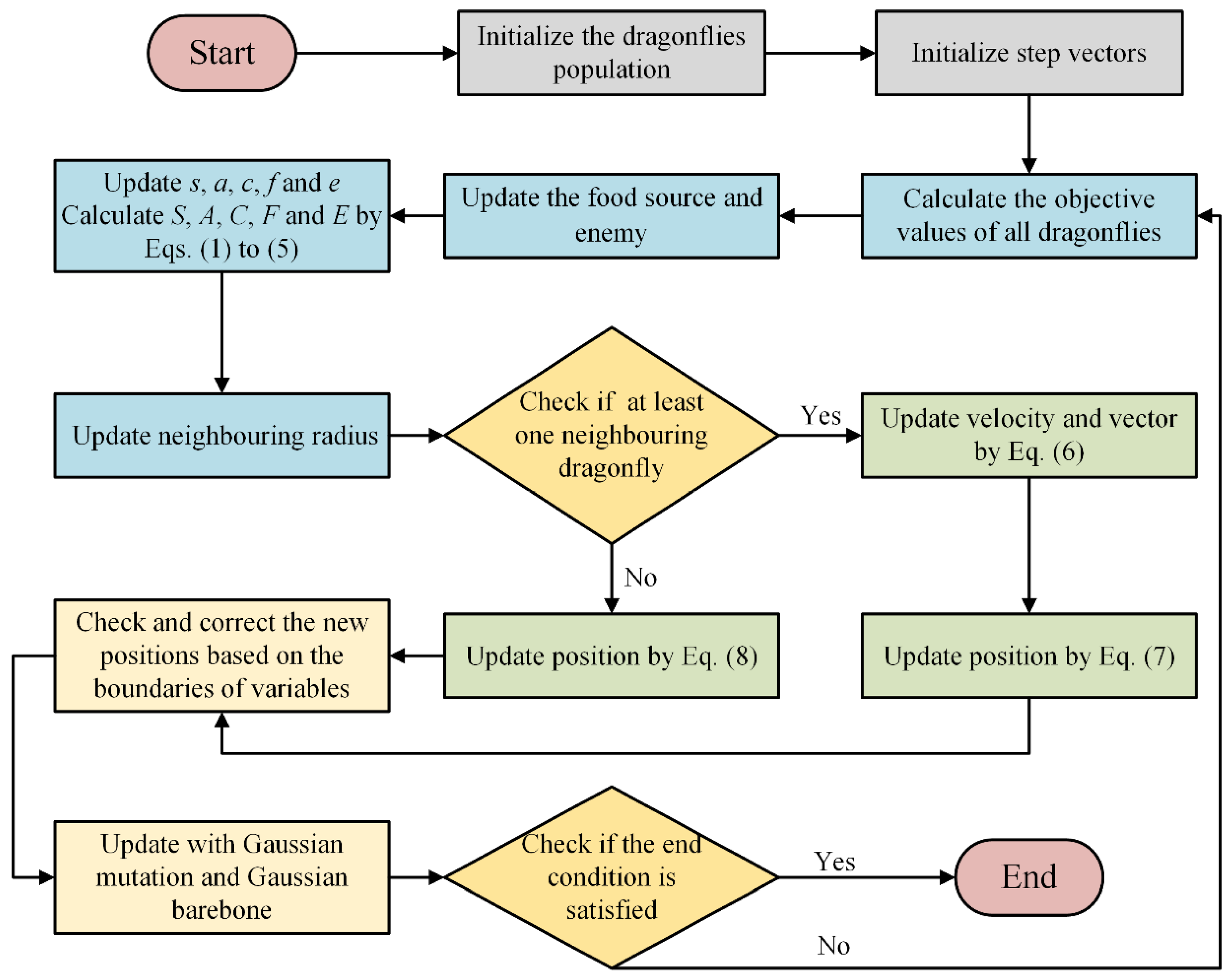
3. Proposed Method
| Algorithm 1. Pseudocode of GGBDA |
| Begin Initialize the dragonflies’ population Initialize the step vectors while the end condition is not satisfied Calculate the population fitness of all the dragonflies Update the food source and enemy Update w, s, a, c, f, and e Calculate S, A, C, F, and E by Equations (1)–(5) Update the neighboring radius if a dragonfly has at least one neighboring dragonfly Update the velocity and vector by Equation (6) Update the position vector by Equation (7) else Update the position vector by Equation (8) end if Check and correct the new position according to the boundaries of the variables Update with the Gaussian mutation and Gaussian barebone end while End |
4. Experimental Results
4.1. Benchmark Functions
4.2. Comparison with Classical Algorithms
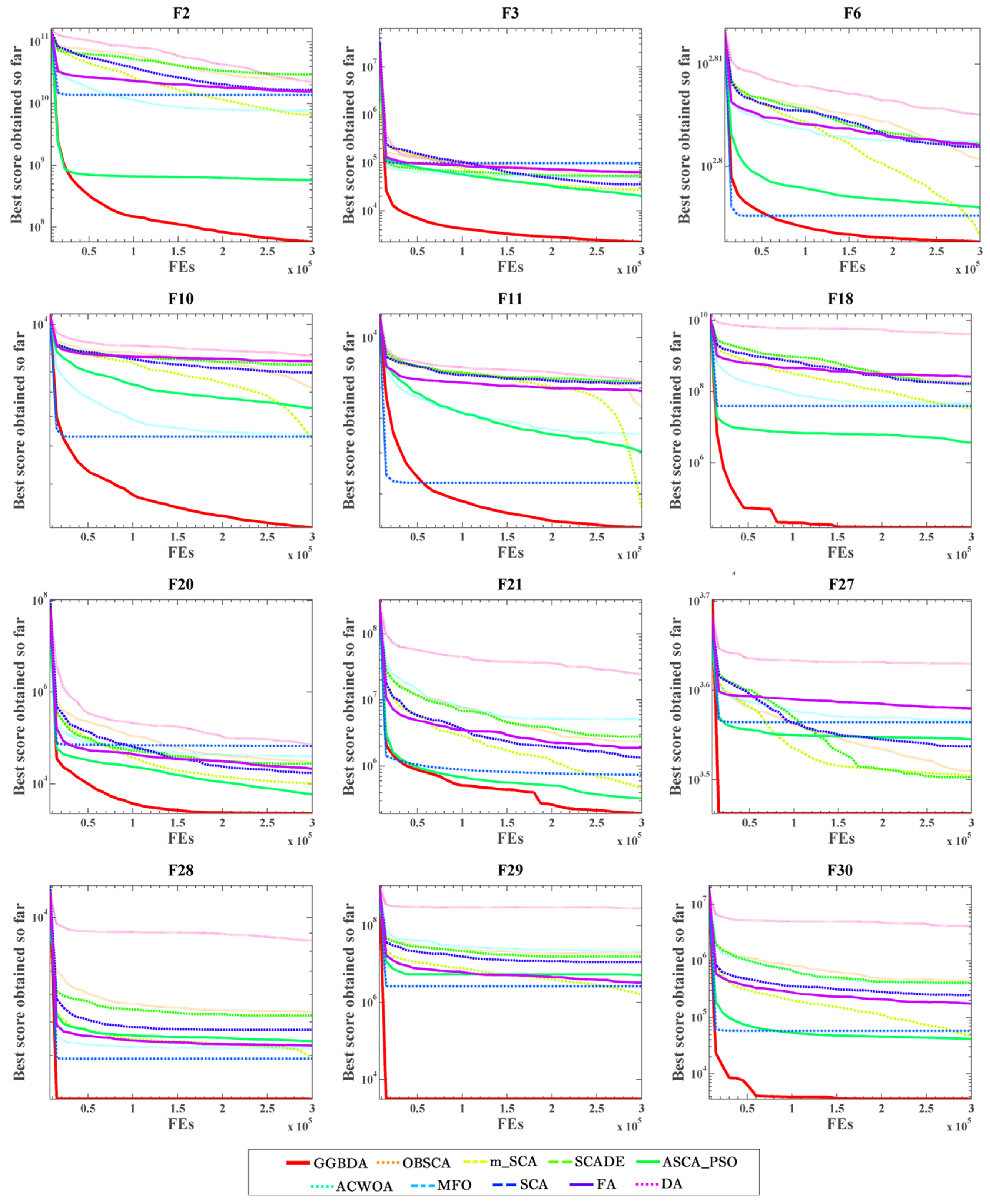
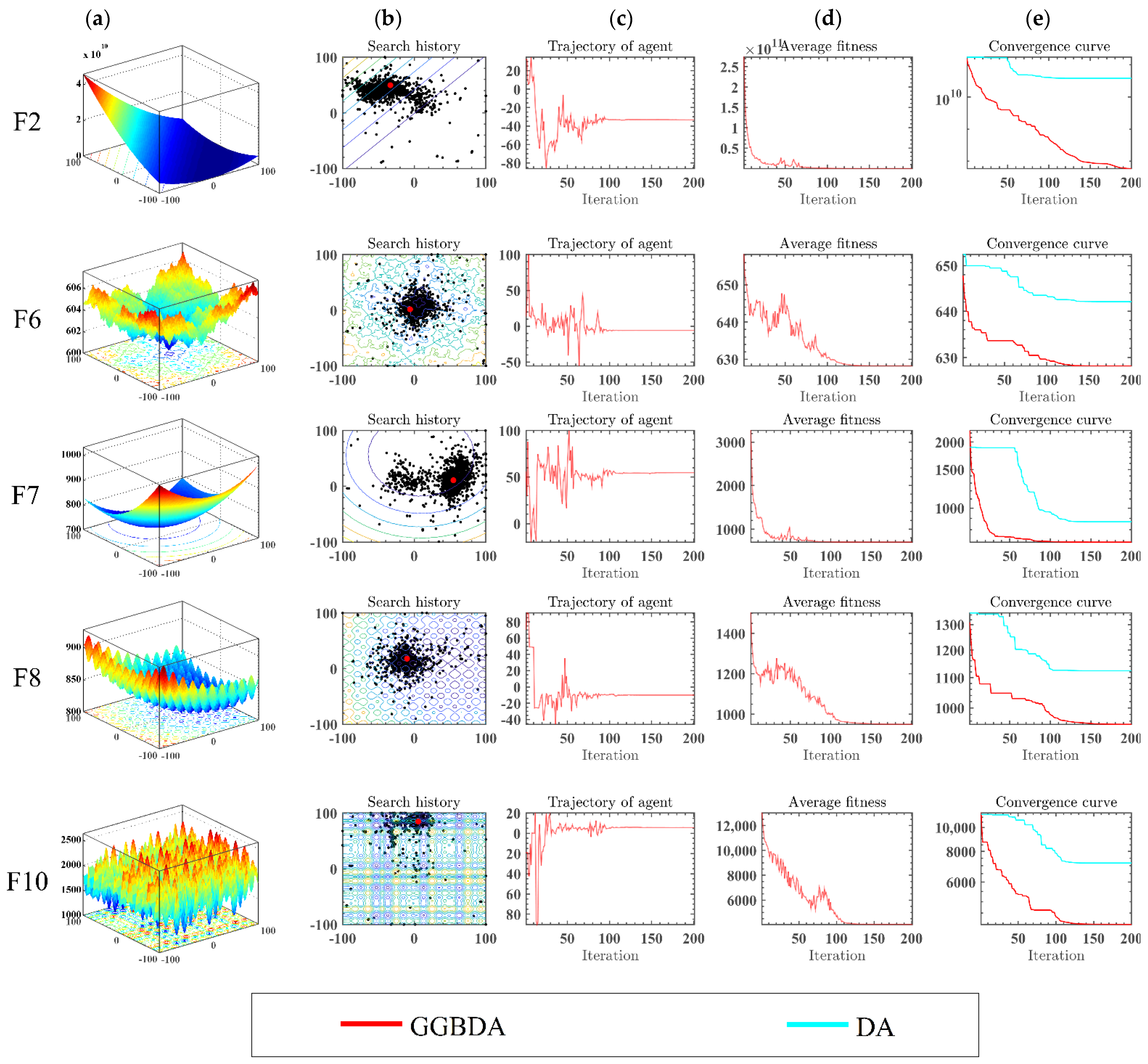
4.2.1. Results on 30D Functions
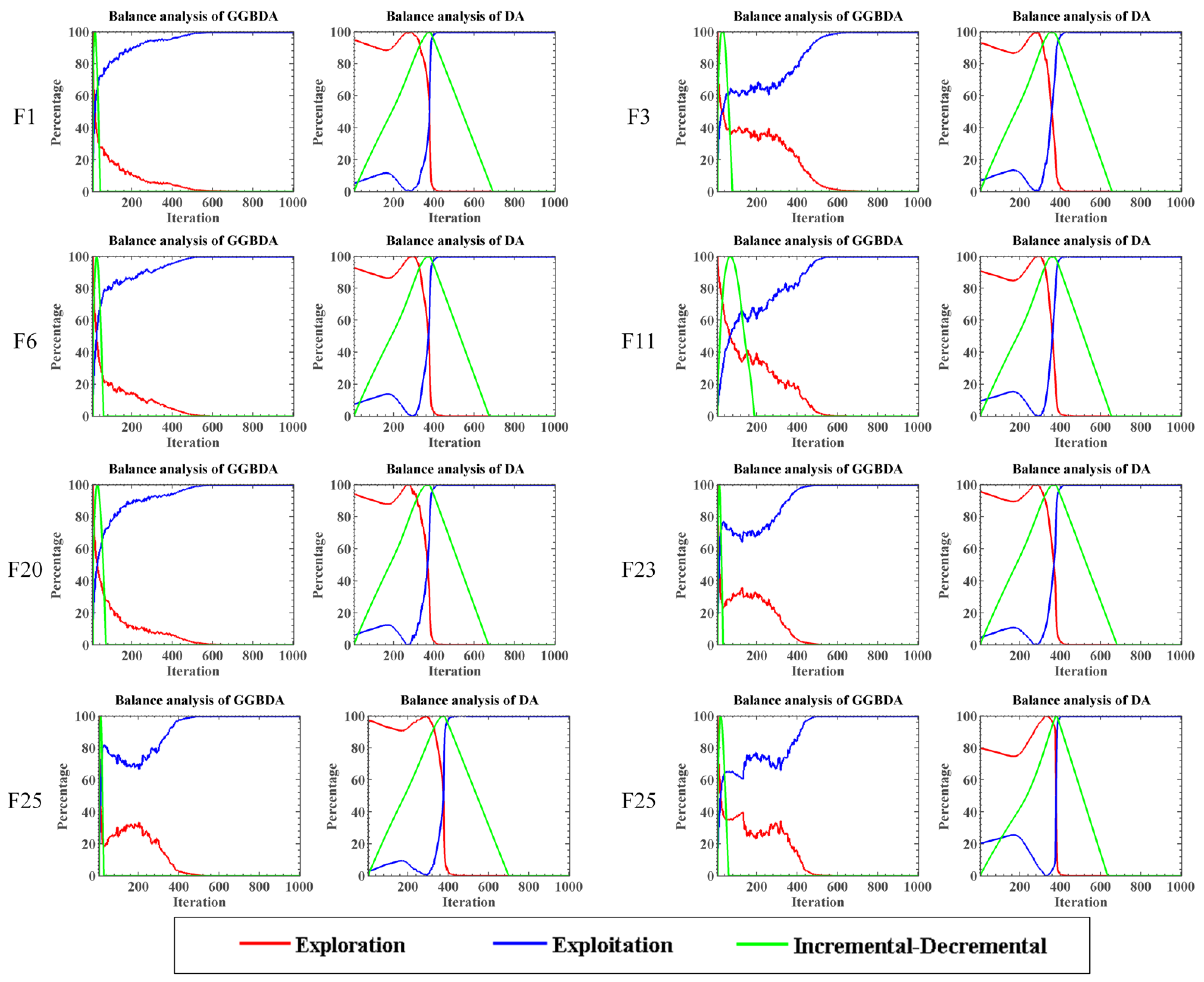
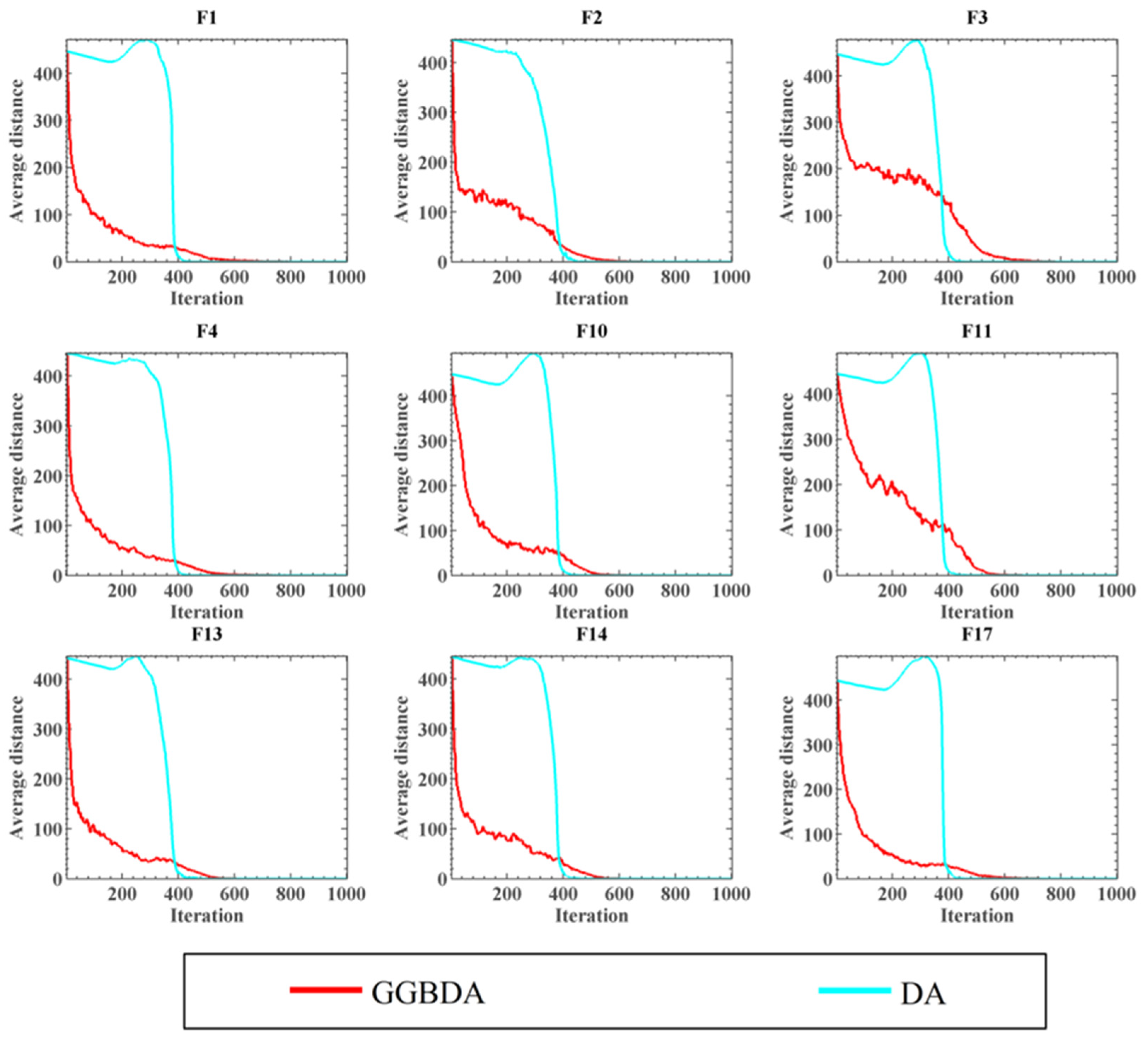
4.2.2. Balance Analysis
4.3. Real-World Problems
4.3.1. Pressure Vessel Design (PVD) Problem
4.3.2. Hydrostatic Thrust Bearings Design (HTBD) Problem
4.3.3. Welded Beam Design (WBD) Problem
4.3.4. Tension–Compression String Design (TCSD) Problem
5. Conclusions
Author Contributions
Funding
Data Availability Statement
Conflicts of Interest
References
- Zhan, Z.H.; Shi, L.; Tan, K.C.; Zhang, J. A survey on evolutionary computation for complex continuous optimization. Artif. Intell. Rev. 2021, 55, 59–110. [Google Scholar] [CrossRef]
- Mirjalili, S.; Lewis, A. The Whale Optimization Algorithm. Adv. Eng. Softw. 2016, 95, 51–67. [Google Scholar] [CrossRef]
- Luo, J.; Chen, H.; Heidari, A.A.; Xu, Y.; Zhang, Q.; Li, C. Multi-strategy boosted mutative whale-inspired optimization approaches. Appl. Math. Model. 2019, 73, 109–123. [Google Scholar] [CrossRef]
- Storn, R.; Price, K. Differential Evolution—A Simple and Efficient Heuristic for Global Optimization over Continuous Spaces. J. Glob. Optim. 1997, 11, 341–359. [Google Scholar] [CrossRef]
- Booker, L.B.; Goldberg, D.E.; Holland, J.H. Classifier systems and genetic algorithms. Artif. Intell. 1989, 40, 235–282. [Google Scholar] [CrossRef]
- Dorigo, M.; Maniezzo, V.; Colorni, A. Ant system: Optimization by a colony of cooperating agents. IEEE Trans. Syst. Man Cybern. Part B 1996, 26, 29–41. [Google Scholar] [CrossRef] [Green Version]
- Deng, W.; Xu, J.; Zhao, H. An Improved Ant Colony Optimization Algorithm Based on Hybrid Strategies for Scheduling Problem. IEEE Access 2019, 7, 20281–20292. [Google Scholar] [CrossRef]
- Kennedy, J.; Eberhart, R. Particle swarm optimization. In Proceedings of the IEEE International Conference on Neural Networks—Conference Proceedings, Perth, WA, Australia, 27 November–1 December 1995; IEEE: Piscataway, NJ, USA, 1995. [Google Scholar]
- Zhang, X.; Hu, W.; Xie, N.; Bao, H.; Maybank, S. A Robust Tracking System for Low Frame Rate Video. Int. J. Comput. Vis. 2015, 115, 279–304. [Google Scholar] [CrossRef] [Green Version]
- Yang, X.-S. Firefly Algorithms for Multimodal Optimization. In Stochastic Algorithms: Foundations and Applications; SAGA 2009. Lecture Notes in Computer Science; Springer: Berlin/Heidelberg, Germany, 2010; Volume 5792. [Google Scholar]
- Pan, W.T. A new Fruit Fly Optimization Algorithm: Taking the financial distress model as an example. Knowl.-Based Syst. 2012, 26, 69–74. [Google Scholar] [CrossRef]
- Shen, L.; Chen, H.; Yu, Z.; Kang, W.; Zhang, B.; Li, H.; Yang, B.; Liu, D. Evolving support vector machines using fruit fly optimization for medical data classification. Knowl.-Based Syst. 2016, 96, 61–75. [Google Scholar] [CrossRef]
- Zhang, Y.; Liu, R.; Asghar Heidari, A.; Wang, X.; Chen, Y.; Wang, M.; Chen, H. Towards Augmented Kernel Extreme Learning Models for Bankruptcy Prediction: Algorithmic Behavior and Comprehensive Analysis. Neurocomputing 2020, 430, 185–212. [Google Scholar] [CrossRef]
- Li, S.; Chen, H.; Wang, M.; Heidari, A.A.; Mirjalili, S. Slime mould algorithm: A new method for stochastic optimization. Future Gener. Comput. Syst. 2020, 111, 300–323. [Google Scholar] [CrossRef]
- Mirjalili, S. Moth-flame optimization algorithm: A novel nature-inspired heuristic paradigm. Knowl.-Based Syst. 2015, 89, 228–249. [Google Scholar] [CrossRef]
- Xu, Y.; Chen, H.; Luo, J.; Zhang, Q.; Jiao, S.; Zhang, X. Enhanced Moth-flame optimizer with mutation strategy for global optimization. Inf. Sci. 2019, 492, 181–203. [Google Scholar] [CrossRef]
- Xu, Y.; Chen, H.; Heidari, A.A.; Luo, J.; Zhang, Q.; Zhao, X.; Li, C. An efficient chaotic mutative moth-flame-inspired optimizer for global optimization tasks. Expert Syst. Appl. 2019, 129, 135–155. [Google Scholar] [CrossRef]
- Mirjalili, S.; Mirjalili, S.M.; Lewis, A. Grey Wolf Optimizer. Adv. Eng. Softw. 2014, 69, 46–61. [Google Scholar] [CrossRef] [Green Version]
- Zhao, X.; Zhang, X.; Cai, Z.; Tian, X.; Wang, X.; Huang, Y.; Chen, H.; Hu, L. Chaos enhanced grey wolf optimization wrapped ELM for diagnosis of paraquat-poisoned patients. Comput. Biol. Chem. 2019, 78, 481–490. [Google Scholar] [CrossRef]
- Yang, X.S. A new metaheuristic Bat-inspired Algorithm. In Nature Inspired Cooperative Strategies for Optimization (NICSO 2010); (Studies in Computational Intelligence); Springer: Berlin/Heidelberg, Germany, 2010; pp. 65–74. [Google Scholar]
- Yu, H.; Zhao, N.; Wang, P.; Chen, H.; Li, C. Chaos-enhanced synchronized bat optimizer. Appl. Math. Model. 2020, 77, 1201–1215. [Google Scholar] [CrossRef]
- Saremi, S.; Mirjalili, S.; Lewis, A. Grasshopper Optimisation Algorithm: Theory and application. Adv. Eng. Softw. 2017, 105, 30–47. [Google Scholar] [CrossRef] [Green Version]
- Luo, J.; Chen, H.; Zhang, Q.; Xu, Y.; Huang, H.; Zhao, X. An improved grasshopper optimization algorithm with application to financial stress prediction. Appl. Math. Model. 2018, 64, 654–668. [Google Scholar] [CrossRef]
- Heidari, A.A.; Mirjalili, S.; Faris, H.; Aljarah, I.; Mafarja, M.; Chen, H. Harris hawks optimization: Algorithm and applications. Future Gener. Comput. Syst. 2019, 97, 849–872. [Google Scholar] [CrossRef]
- Tu, J.; Chen, H.; Wang, M.; Gandomi, A.H. The Colony Predation Algorithm. J. Bionic Eng. 2021, 18, 674–710. [Google Scholar] [CrossRef]
- Yang, Y.; Chen, H.; Heidari, A.A.; Gandomi, A.H. Hunger games search: Visions, conception, implementation, deep analysis, perspectives, and towards performance shifts. Expert Syst. Appl. 2021, 177, 114864. [Google Scholar] [CrossRef]
- Ahmadianfar, I.; Asghar Heidari, A.; Gandomi, A.H.; Chu, X.; Chen, H. RUN Beyond the Metaphor: An Efficient Optimization Algorithm Based on Runge Kutta Method. Expert Syst. Appl. 2021, 181, 115079. [Google Scholar] [CrossRef]
- Ahmadianfar, I.; Asghar Heidari, A.; Noshadian, S.; Chen, H.; Gandomi, A.H. INFO: An Efficient Optimization Algorithm based on Weighted Mean of Vectors. Expert Syst. Appl. 2022, 194, 116516. [Google Scholar] [CrossRef]
- Wu, S.-H.; Zhan, Z.-H.; Zhang, J. SAFE: Scale-adaptive fitness evaluation method for expensive optimization problems. IEEE Trans. Evol. Comput. 2021, 25, 478–491. [Google Scholar] [CrossRef]
- Li, J.-Y.; Zhan, Z.-H.; Wang, C.; Jin, H.; Zhang, J. Boosting data-driven evolutionary algorithm with localized data generation. IEEE Trans. Evol. Comput. 2020, 24, 923–937. [Google Scholar] [CrossRef]
- Ying, C.; Ying, C.; Ban, C. A performance optimization strategy based on degree of parallelism and allocation fitness. EURASIP J. Wirel. Commun. Netw. 2018, 2018, 1–8. [Google Scholar] [CrossRef] [Green Version]
- Hu, K.; Ye, J.; Fan, E.; Shen, S.; Huang, L.; Pi, J. A novel object tracking algorithm by fusing color and depth information based on single valued neutrosophic cross-entropy. J. Intell. Fuzzy Syst. 2017, 32, 1775–1786. [Google Scholar] [CrossRef] [Green Version]
- Hu, K.; He, W.; Ye, J.; Zhao, L.; Peng, H.; Pi, J. Online Visual Tracking of Weighted Multiple Instance Learning via Neutrosophic Similarity-Based Objectness Estimation. Symmetry 2019, 11, 832. [Google Scholar] [CrossRef] [Green Version]
- Zhang, W.; Hou, W.; Li, C.; Yang, W.; Gen, M. Multidirection Update-Based Multiobjective Particle Swarm Optimization for Mixed No-Idle Flow-Shop Scheduling Problem. Complex Syst. Modeling Simul. 2021, 1, 176–197. [Google Scholar] [CrossRef]
- Liu, X.-F.; Zhan, Z.-H.; Gao, Y.; Zhang, J.; Kwong, S.; Zhang, J. Coevolutionary particle swarm optimization with bottleneck objective learning strategy for many-objective optimization. IEEE Trans. Evol. Comput. 2018, 23, 587–602. [Google Scholar] [CrossRef]
- Deng, W.; Zhang, X.; Zhou, Y.; Liu, Y.; Deng, W.; Chen, H.; Zhao, H. An enhanced fast non-dominated solution sorting genetic algorithm for multi-objective problems. Inf. Sci. 2021, 585, 441–453. [Google Scholar] [CrossRef]
- Lai, X.; Zhou, Y. Analysis of multiobjective evolutionary algorithms on the biobjective traveling salesman problem (1, 2). Multimed. Tools Appl. 2020, 79, 30839–30860. [Google Scholar] [CrossRef]
- Yang, Z.; Li, K.; Guo, Y.; Ma, H.; Zheng, M. Compact real-valued teaching-learning based optimization with the applications to neural network training. Knowl. Based Syst. 2018, 159, 51–62. [Google Scholar] [CrossRef]
- Han, X.; Han, Y.; Chen, Q.; Li, J.; Sang, H.; Liu, Y.; Pan, Q.; Nojima, Y. Distributed Flow Shop Scheduling with Sequence-Dependent Setup Times Using an Improved Iterated Greedy Algorithm. Complex Syst. Modeling Simul. 2021, 1, 198–217. [Google Scholar] [CrossRef]
- Yi, J.-H.; Deb, S.; Dong, J.; Alavi, A.H.; Wang, G.-G. An improved NSGA-III algorithm with adaptive mutation operator for Big Data optimization problems. Future Gener. Comput. Syst. 2018, 88, 571–585. [Google Scholar] [CrossRef]
- Deng, W.; Liu, H.; Xu, J.; Zhao, H.; Song, Y.J. An improved quantum-inspired differential evolution algorithm for deep belief network. IEEE Trans. Instrum. Meas. 2020, 69, 7319–7327. [Google Scholar] [CrossRef]
- Sun, Y.; Xue, B.; Zhang, M.; Yen, G.G. Evolving deep convolutional neural networks for image classification. IEEE Trans. Evol. Comput. 2019, 24, 394–407. [Google Scholar] [CrossRef] [Green Version]
- Deng, W.; Xu, J.; Zhao, H.; Song, Y. A Novel Gate Resource Allocation Method Using Improved PSO-Based QEA. IEEE Trans. Intell. Transp. Syst. 2020. [Google Scholar] [CrossRef]
- Deng, W.; Xu, J.; Song, Y.; Zhao, H. An Effective Improved Co-evolution Ant Colony Optimization Algorithm with Multi-Strategies and Its Application. Int. J. Bio-Inspired Comput. 2020, 16, 158–170. [Google Scholar] [CrossRef]
- Zhao, F.; Di, S.; Cao, J.; Tang, J. A novel cooperative multi-stage hyper-heuristic for combination optimization problems. Complex Syst. Modeling Simul. 2021, 1, 91–108. [Google Scholar] [CrossRef]
- Mirjalili, S. Dragonfly algorithm: A new meta-heuristic optimization technique for solving single-objective, discrete, and multi-objective problems. Neural Comput. Appl. 2016, 27, 1053–1073. [Google Scholar] [CrossRef]
- Guha, D.; Roy, P.K.; Banerjee, S. Optimal tuning of 3 degree-of-freedom proportional-integral-derivative controller for hybrid distributed power system using dragonfly algorithm. Comput. Electr. Eng. 2018, 72, 137–153. [Google Scholar] [CrossRef]
- Wu, J.; Zhu, Y.; Wang, Z.; Song, Z.; Liu, X.; Wang, W.; Zhang, Z.; Yu, Y.; Xu, Z.; Zhang, T.; et al. A novel ship classification approach for high resolution SAR images based on the BDA-KELM classification model. Int. J. Remote Sens. 2017, 38, 6457–6476. [Google Scholar] [CrossRef]
- Ashok Kumar, C.; Vimala, R.; Aravind Britto, K.R.; Sathya Devi, S. FDLA: Fractional Dragonfly based Load balancing Algorithm in cluster cloud model. Clust. Comput. 2019, 22, 1401–1414. [Google Scholar] [CrossRef]
- VeeraManickam, M.R.M.; Mohanapriya, M.; Pandey, B.K.; Akhade, S.; Kale, S.A.; Patil, R.; Vigneshwar, M. Map-Reduce framework based cluster architecture for academic student’s performance prediction using cumulative dragonfly based neural network. Clust. Comput. 2019, 22, 1259–1275. [Google Scholar] [CrossRef]
- Yu, C.; Cai, Z.; Ye, X.; Wang, M.; Zhao, X.; Liang, G.; Chen, H.; Li, C. Quantum-like mutation-induced dragonfly-inspired optimization approach. Math. Comput. Simul. 2020, 178, 259–289. [Google Scholar] [CrossRef]
- Sree Ranjini, S.R.; Murugan, S. Memory based Hybrid Dragonfly Algorithm for numerical optimization problems. Expert Syst. Appl. 2017, 83, 63–78. [Google Scholar]
- More, N.S.; Ingle, R.B. Energy-aware VM migration using dragonfly-crow optimization and support vector regression model in Cloud. Int. J. Modeling Simul. Sci. Comput. 2018, 9, 1850050. [Google Scholar] [CrossRef]
- Khadanga, R.K.; Padhy, S.; Panda, S.; Kumar, A. Design and Analysis of Tilt Integral Derivative Controller for Frequency Control in an Islanded Microgrid: A Novel Hybrid Dragonfly and Pattern Search Algorithm Approach. Arab. J. Sci. Eng. 2018, 43, 3103–3114. [Google Scholar] [CrossRef]
- Ghanem, W.A.H.M.; Jantan, A. A Cognitively Inspired Hybridization of Artificial Bee Colony and Dragonfly Algorithms for Training Multi-layer Perceptrons. Cogn. Comput. 2018, 10, 1096–1134. [Google Scholar] [CrossRef]
- Shilaja, C.; Arunprasath, T. Internet of medical things-load optimization of power flow based on hybrid enhanced grey wolf optimization and dragonfly algorithm. Future Gener. Comput. Syst. 2019, 98, 319–330. [Google Scholar]
- Aadil, F.; Ahsan, W.; Rehman, Z.U.; Shah, P.A.; Rho, S.; Mehmood, I. Clustering algorithm for internet of vehicles (IoV) based on dragonfly optimizer (CAVDO). J. Supercomput. 2018, 74, 4542–4567. [Google Scholar] [CrossRef]
- Aci, C.I.; Gülcan, H. A modified dragonfly optimization algorithm for single- and multiobjective problems using brownian motion. Comput. Intell. Neurosci. 2019, 2019, 6871298. [Google Scholar] [CrossRef] [PubMed] [Green Version]
- Bao, X.; Jia, H.; Lang, C. Dragonfly algorithm with Opposition-based learning for multilevel thresholding color image segmentation. Symmetry 2019, 11, 716. [Google Scholar] [CrossRef] [Green Version]
- Li, L.L.; Zhao, X.; Tseng, M.L.; Tan, R.R. Short-term wind power forecasting based on support vector machine with improved dragonfly algorithm. J. Clean. Prod. 2020, 242, 118447. [Google Scholar] [CrossRef]
- Sayed, G.I.; Tharwat, A.; Hassanien, A.E. Chaotic dragonfly algorithm: An improved metaheuristic algorithm for feature selection. Appl. Intell. 2019, 49, 188–205. [Google Scholar] [CrossRef]
- Mafarja, M.; Aljarah, I.; Heidari, A.A.; Faris, H.; Fournier-Viger, P.; Li, X.; Mirjalili, S. Binary dragonfly optimization for feature selection using time-varying transfer functions. Knowl.-Based Syst. 2018, 161, 185–204. [Google Scholar] [CrossRef]
- Hariharan, M.; Sindhu, R.; Vijean, V.; Yazid, H.; Nadarajaw, T.; Yaacob, S.; Polat, K. Improved binary dragonfly optimization algorithm and wavelet packet based non-linear features for infant cry classification. Comput. Methods Programs Biomed. 2018, 155, 39–51. [Google Scholar] [CrossRef]
- Zhang, A.; Zhang, P.; Feng, Y. Short-term load forecasting for microgrids based on DA-SVM. COMPEL Int. J. Comput. Math. Electr. Electron. Eng. 2018, 38, 68–80. [Google Scholar] [CrossRef]
- Yuan, Y.; Lv, L.; Wang, X.; Song, X. Optimization of a frame structure using the Coulomb force search strategy-based dragonfly algorithm. Eng. Optim. 2019, 52, 915–931. [Google Scholar] [CrossRef]
- Zhang, Z.; Hong, W.C. Electric load forecasting by complete ensemble empirical mode decomposition adaptive noise and support vector regression with quantum-based dragonfly algorithm. Nonlinear Dyn. 2019, 98, 1107–1136. [Google Scholar] [CrossRef]
- Suresh, V.; Sreejith, S. Generation dispatch of combined solar thermal systems using dragonfly algorithm. Computing 2017, 99, 59–80. [Google Scholar] [CrossRef]
- Sureshkumar, K.; Ponnusamy, V. Power flow management in micro grid through renewable energy sources using a hybrid modified dragonfly algorithm with bat search algorithm. Energy 2019, 181, 1166–1178. [Google Scholar] [CrossRef]
- Xie, T.; Yao, J.; Zhou, Z. DA-based parameter optimization of combined kernel support vector machine for cancer diagnosis. Processes 2019, 7, 263. [Google Scholar] [CrossRef] [Green Version]
- Xu, L.; Jia, H.; Lang, C.; Peng, X.; Sun, K. A Novel Method for Multilevel Color Image Segmentation Based on Dragonfly Algorithm and Differential Evolution. IEEE Access 2019, 7, 19502–19538. [Google Scholar] [CrossRef]
- Zhang, Q.; Wang, Z.; Heidari, A.A.; Gui, W.; Shao, Q.; Chen, H.; Zaguia, A.; Turabieh, H.; Chen, M. Gaussian Barebone Salp Swarm Algorithm with Stochastic Fractal Search for medical image segmentation: A COVID-19 case study. Comput. Biol. Med. 2021, 139, 104941. [Google Scholar] [CrossRef]
- Xia, J.; Zhang, H.; Li, R.; Wang, Z.; Cai, Z.; Gu, Z.; Chen, H.; Pan, Z. Adaptive Barebones Salp Swarm Algorithm with Quasi-oppositional Learning for Medical Diagnosis Systems: A Comprehensive Analysis. J. Bionic Eng. 2022, 19, 1–17. [Google Scholar] [CrossRef]
- Liang, J.; Qu, B.Y.; Suganthan, P. Problem Definitions and Evaluation Criteria for the CEC 2014 Special Session and Competition on Single Objective Real-Parameter Numerical Optimization; Technical Report, 201311; Zhengzhou University: Zhengzhou, China; Nanyang Technological University: Singapore, 2013. [Google Scholar]
- Abd Elaziz, M.; Oliva, D.; Xiong, S. An improved Opposition-Based Sine Cosine Algorithm for global optimization. Expert Syst. Appl. 2017, 90, 484–500. [Google Scholar] [CrossRef]
- Qu, C.; Zeng, Z.; Dai, J.; Yi, Z.; He, W. A Modified Sine-Cosine Algorithm Based on Neighborhood Search and Greedy Levy Mutation. Comput. Intell. Neurosci. 2018, 2018, 4231647. [Google Scholar] [CrossRef] [PubMed]
- Nenavath, H.; Jatoth, R.K. Hybridizing sine cosine algorithm with differential evolution for global optimization and object tracking. Appl. Soft Comput. 2018, 62, 1019–1043. [Google Scholar] [CrossRef]
- Issa, M.; Hassanien, A.E.; Oliva, D.; Helmi, A.; Ziedan, I.; Alzohairy, A. ASCA-PSO: Adaptive sine cosine optimization algorithm integrated with particle swarm for pairwise local sequence alignment. Expert Syst. Appl. 2018, 99, 56–70. [Google Scholar] [CrossRef]
- Elhosseini, M.A.; Haikal, A.Y.; Badawy, M.; Khashan, N. Biped robot stability based on an A–C parametric Whale Optimization Algorithm. J. Comput. Sci. 2019, 31, 17–32. [Google Scholar] [CrossRef]
- Mirjalili, S. SCA: A Sine Cosine Algorithm for solving optimization problems. Knowl.-Based Syst. 2016, 96, 120–133. [Google Scholar] [CrossRef]
- Yang, X.-S. Firefly Algorithms for Multimodal Optimization; Springer: Berlin/Heidelberg, Germany, 2009. [Google Scholar]
- Cui, H.; Guan, Y.; Chen, H.; Deng, W. A Novel Advancing Signal Processing Method Based on Coupled Multi-Stable Stochastic Resonance for Fault Detection. Appl. Sci. 2021, 11, 5385. [Google Scholar] [CrossRef]
- Fu, J.; Zhang, Y.; Wang, Y.; Zhang, H.; Liu, J.; Tang, J.; Yang, Q.; Sun, H.; Qiu, W.; Ma, Y. Optimization of metabolomic data processing using NOREVA. Nat. Protoc. 2021, 17, 129–151. [Google Scholar] [CrossRef]
- Li, B.; Tang, J.; Yang, Q.; Li, S.; Cui, X.; Li, Y.; Chen, Y.; Xue, W.; Li, X.; Zhu, F. NOREVA: Normalization and evaluation of MS-based metabolomics data. Nucleic Acids Res. 2017, 45, W162–W170. [Google Scholar] [CrossRef] [Green Version]
- Ran, X.; Zhou, X.; Lei, M.; Tepsan, W.; Deng, W. A novel k-means clustering algorithm with a noise algorithm for capturing urban hotspots. Appl. Sci. 2021, 11, 11202. [Google Scholar] [CrossRef]
- Wang, M.; Zhang, Q.; Chen, H.; Heidari, A.A.; Mafarja, M.; Turabieh, H. Evaluation of constraint in photovoltaic cells using ensemble multi-strategy shuffled frog leading algorithms. Energy Convers. Manag. 2021, 244, 114484. [Google Scholar] [CrossRef]
- Yang, Q.; Li, B.; Tang, J.; Cui, X.; Wang, Y.; Li, X.; Hu, J.; Chen, Y.; Xue, W.; Lou, Y. Consistent gene signature of schizophrenia identified by a novel feature selection strategy from comprehensive sets of transcriptomic data. Brief. Bioinform. 2020, 21, 1058–1068. [Google Scholar] [CrossRef] [PubMed]
- Li, Y.H.; Li, X.X.; Hong, J.J.; Wang, Y.X.; Fu, J.B.; Yang, H.; Yu, C.Y.; Li, F.C.; Hu, J.; Xue, W.W. Clinical trials, progression-speed differentiating features and swiftness rule of the innovative targets of first-in-class drugs. Brief. Bioinform. 2020, 21, 649–662. [Google Scholar] [CrossRef] [PubMed] [Green Version]
- Zhu, F.; Qin, C.; Tao, L.; Liu, X.; Shi, Z.; Ma, X.; Jia, J.; Tan, Y.; Cui, C.; Lin, J. Clustered patterns of species origins of nature-derived drugs and clues for future bioprospecting. Proc. Natl. Acad. Sci. USA 2011, 108, 12943–12948. [Google Scholar] [CrossRef] [Green Version]
- Yin, J.; Sun, W.; Li, F.; Hong, J.; Li, X.; Zhou, Y.; Lu, Y.; Liu, M.; Zhang, X.; Chen, N. VARIDT 1.0: Variability of drug transporter database. Nucleic Acids Res. 2020, 48, D1042–D1050. [Google Scholar] [CrossRef]
- Xue, X.; Wang, S.F.; Zhan, L.J.; Feng, Z.Y.; Guo, Y.D. Social Learning Evolution (SLE): Computational Experiment-Based Modeling Framework of Social Manufacturing. IEEE Trans. Ind. Inform. 2019, 15, 3343–3355. [Google Scholar] [CrossRef]
- Xue, X.; Chen, Z.; Wang, S.; Feng, Z.; Duan, Y.; Zhou, Z. Value Entropy: A Systematic Evaluation Model of Service Ecosystem Evolution. IEEE Trans. Serv. Comput. 2020. [Google Scholar] [CrossRef]
- Wu, Z.; Li, R.; Xie, J.; Zhou, Z.; Guo, J.; Xu, X. A user sensitive subject protection approach for book search service. J. Assoc. Inf. Sci. Technol. 2020, 71, 183–195. [Google Scholar] [CrossRef]
- Wu, Z.; Shen, S.; Lian, X.; Su, X.; Chen, E. A dummy-based user privacy protection approach for text information retrieval. Knowl.-Based Syst. 2020, 195, 105679. [Google Scholar] [CrossRef]
- Wu, Z.; Shen, S.; Zhou, H.; Li, H.; Lu, C.; Zou, D. An effective approach for the protection of user commodity viewing privacy in e-commerce website. Knowl.-Based Syst. 2021, 220, 106952. [Google Scholar] [CrossRef]
- Qiu, S.; Hao, Z.; Wang, Z.; Liu, L.; Liu, J.; Zhao, H.; Fortino, G. Sensor Combination Selection Strategy for Kayak Cycle Phase Segmentation Based on Body Sensor Networks. IEEE Internet Things J. 2021, in press. [Google Scholar] [CrossRef]
- Zhang, L.; Zou, Y.; Wang, W.; Jin, Z.; Su, Y.; Chen, H. Resource Allocation and Trust Computing for Blockchain-Enabled Edge Computing System. Comput. Secur. 2021, 105, 102249. [Google Scholar] [CrossRef]
- Zhang, L.; Zhang, Z.; Wang, W.; Waqas, R.; Zhao, C.; Kim, S.; Chen, H. A Covert Communication Method Using Special Bitcoin Addresses Generated by Vanitygen. Comput. Mater. Contin. 2020, 65, 597–616. [Google Scholar]
- Zhang, L.; Zhang, Z.; Wang, W.; Jin, Z.; Su, Y.; Chen, H. Research on a Covert Communication Model Realized by Using Smart Contracts in Blockchain Environment. IEEE Syst. J. 2021, in press. [Google Scholar] [CrossRef]
- Wu, Z.; Li, G.; Shen, S.; Cui, Z.; Lian, X.; Xu, G. Constructing dummy query sequences to protect location privacy and query privacy in location-based services. World Wide Web 2021, 24, 25–49. [Google Scholar] [CrossRef]
- Wu, Z.; Wang, R.; Li, Q.; Lian, X.; Xu, G. A location privacy-preserving system based on query range cover-up for location-based services. IEEE Trans. Veh. Technol. 2020, 69, 5244–5254. [Google Scholar] [CrossRef]
- Qiu, S.; Zhao, H.; Jiang, N.; Wu, D.; Song, G.; Zhao, H.; Wang, Z. Sensor network oriented human motion capture via wearable intelligent system. Int. J. Intell. Syst. 2021, 37, 1646–1673. [Google Scholar] [CrossRef]
- Gandomi, A.; Yang, X.-S.; Alavi, A.; Talatahari, S. Bat algorithm for constrained optimization tasks. Neural Comput. Appl. 2013, 22, 1239–1255. [Google Scholar] [CrossRef]
- He, Q.; Wang, L. A Hybrid Particle Swarm Optimization with a Feasibility-based Rule for Constrained Optimization. Appl. Math. Comput. 2007, 186, 1407–1422. [Google Scholar] [CrossRef]
- Kaveh, A.; Talatahari, S. A Novel Heuristic Optimization Method: Charged System Search. Acta Mech. 2010, 213, 267–289. [Google Scholar] [CrossRef]
- He, Q.; Wang, L. An effective co-evolutionary particle swarm optimization for constrained engineering design problems. Eng. Appl. Artif. Intell. 2007, 20, 89–99. [Google Scholar] [CrossRef]
- Kaveh, A.; Talatahari, S. An improved ant colony optimization for constrained engineering design problems. Eng. Comput. 2010, 27, 155–182. [Google Scholar] [CrossRef]
- Mezura-Montes, E.; ACoello Coello, C.; Velázquez-Reyes, J.; Muñoz-Dávila, L. Multiple trial vectors in differential evolution for engineering design. Eng. Optim. 2007, 39, 567–589. [Google Scholar] [CrossRef]
- Sandgren, E. Nonlinear integer and discrete programming in mechanical design. In Proceedings of the International Design Engineering Technical Conferences and Computers and Information in Engineering Conference, Kissimmee, FL, USA, 25–28 September 1988; The American Society of Mechanical Engineers: New York, NY, USA, 1988; Volume 14. [Google Scholar]
- Wagdy, A. A novel differential evolution algorithm for solving constrained engineering optimization problems. J. Intell. Manuf. 2018, 29, 659–692. [Google Scholar]
- Rao, V.R.; Savsani, J.V.; Vakharia, P.D. Teaching–learning-based optimization: A novel method for constrained mechanical design optimization problems. Comput. Aided Des. 2011, 43, 303–315. [Google Scholar] [CrossRef]
- Kentli, A.; Sahbaz, M. Optimisation of Hydrostatic Thrust Bearing Using Sequential Quadratic Programming. Oxid. Commun. 2014, 37, 1144–1152. [Google Scholar]
- He, S.; Prempain, E.; Wu, Q. An improved particle swarm optimizer for mechanical design optimization problems. Eng. Optim. 2004, 36, 585–605. [Google Scholar] [CrossRef]
- Kaveh, A.; Khayatazad, M. A new meta-heuristic method: Ray Optimization. Comput. Struct. 2012, 112–113, 283–294. [Google Scholar] [CrossRef]
- Mirjalili, S.; Gandomi, A.H.; Mirjalili, S.Z.; Saremi, S.; Faris, H.; Mirjalili, S.M. Salp Swarm Algorithm: A bio-inspired optimizer for engineering design problems. Adv. Eng. Softw. 2017, 114, 163–191. [Google Scholar] [CrossRef]
- Huang, F.-Z.; Wang, L.; He, Q. An effective co-evolutionary differential evolution for constrained optimization. Appl. Math. Comput. 2007, 186, 340–356. [Google Scholar] [CrossRef]
- Rashedi, E.; Nezamabadi-Pour, H.; Saryazdi, S. GSA: A Gravitational Search Algorithm. Inf. Sci. 2009, 179, 2232–2248. [Google Scholar] [CrossRef]
- Coello Coello, C.A. Use of a self-adaptive penalty approach for engineering optimization problems. Comput. Ind. 2000, 41, 113–127. [Google Scholar] [CrossRef]
- Sandgren, E. Nonlinear Integer and Discrete Programming in Mechanical Design Optimization. J. Mech. Des. 1990, 112, 223–229. [Google Scholar] [CrossRef]
- Mezura-Montes, E.; Coello, C.A.C. An empirical study about the usefulness of evolution strategies to solve constrained optimization problems. Int. J. Gen. Syst. 2008, 37, 443–473. [Google Scholar] [CrossRef]


| ID | Function Equation | Search Range | Optimum Value |
|---|---|---|---|
| CEC 2014 Unimodal Functions | |||
| F1 | Rotated High Conditioned Elliptic Function | [−100,100] | |
| F2 | Rotated Bent Cigar Function | [−100,100] | |
| F3 | Rotated Discus Function | [−100,100] | |
| CEC 2014 Simple Multi-Modal Functions | |||
| F4 | Shifted and Rotated Rosenbrock Function | [−100,100] | |
| F5 | Shifted and Rotated Ackley Function | [−100,100] | |
| F6 | Shifted and Rotated Weierstrass Function | [−100,100] | |
| F7 | Shifted and Rotated Griewank Function | [−100,100] | |
| F8 | Shifted Rastrigin Function | [−100,100] | |
| F9 | Shifted and Rotated Rastrigin Function | [−100,100] | |
| F10 | Shifted Schwefel Function | [−100,100] | |
| F11 | Shifted and Rotated Schwefel Function | [−100,100] | |
| F12 | Shifted and Rotated Katsuura Function | [−100,100] | |
| F13 | Shifted and Rotated HappyCat Function | [−100,100] | |
| F14 | Shifted and Rotated HGBat Function | [−100,100] | |
| F15 | Shifted and Rotated Expanded Griewank Plus Rosenbrock Function | [−100,100] | |
| F16 | Shifted and Rotated Expanded Scaffer F6 Function | [−100,100] | |
| CEC 2014 Hybrid Functions | |||
| F17 | Hybrid Function 1 (N = 3) | [−100,100] | |
| F18 | Hybrid Function 2 (N = 3) | [−100,100] | |
| F19 | Hybrid Function 3 (N = 4) | [−100,100] | |
| F20 | Hybrid Function 4 (N = 4) | [−100,100] | |
| F21 | Hybrid Function 5 (N = 5) | [−100,100] | |
| F22 | Hybrid Function 6 (N = 5) | [−100,100] | |
| CEC 2014 Composition Functions | |||
| F23 | Composition Function 1 (N = 5) | [−100,100] | |
| F24 | Composition Function 2 (N = 3) | [−100,100] | |
| F25 | Composition Function 3 (N = 3) | [−100,100] | |
| F26 | Composition Function 4 (N = 5) | [−100,100] | |
| F27 | Composition Function 5 (N = 5) | [−100,100] | |
| F28 | Composition Function 6 (N = 5) | [−100,100] | |
| F29 | Composition Function 7 (N = 3) | [−100,100] | |
| F30 | Composition Function 8 (N = 3) | [−100,100] | |
| Algorithms | Pop | Maximum Iterations | Others |
|---|---|---|---|
| GGBDA OBSCA m_SCA | 30 | 1000 | w ∈ [0.9 0.2]; s = 0.1; a = 0.1; c = 0.7; f = 1; e = 1 |
| 30 | 1000 | a = 2 | |
| 30 | 1000 | a = 2 | |
| SCADE ASCA_PSO | 30 | 1000 | a = 2; CR = 0.8; LSF = 0.8; USF = 0.2 |
| 30 | 1000 | M = 4; N = 9; Vmax = 6; wMax = 0.9; wMin = 0.2; c1 = 2; c2 = 2; | |
| ACWOA MFO SCA FA | 30 | 1000 | B = 1 |
| 30 | 1000 | B = 1 | |
| 30 | 1000 | a = 2 | |
| 30 | 1000 | alpha = 0.5; betamin = 0.2; gamma = 1; | |
| DA GGBDA | 30 | 1000 | w ∈ [0.9 0.2]; s = 0.1; a = 0.1; c = 0.7; f = 1; e = 1 |
| 30 | 1000 | w ∈ [0.9 0.2]; s = 0.1; a = 0.1; c = 0.7; f = 1; e = 1 |
| F1 | F2 | F3 | ||||
| Ave | Std | Ave | Std | Ave | Std | |
| GGBDA | 3.3428 × 10⁷ | 2.3615 × 10⁷ | 5.7799 × 10⁷ | 1.32174 × 10⁷ | 2.2502 × 10³ | 1.0237 × 10³ |
| OBSCA | 3.8095 × 10⁸ | 1.2188 × 10⁸ | 2.4577 × 10¹⁰ | 3.9982 × 10⁹ | 5.1744 × 10⁴ | 7.3043 × 10³ |
| m_SCA | 7.2766 × 10⁷ | 3.9039 × 10⁷ | 6.4809 × 10⁹ | 2.7501 × 10⁹ | 2.6967 × 10⁴ | 7.4237 × 10³ |
| SCADE | 4.3235 × 10⁸ | 1.0258 × 10⁸ | 2.9383 × 10¹⁰ | 4.9065 × 10⁹ | 5.3542 × 10⁴ | 6.3130 × 10³ |
| ASCA_PSO | 1.5733 × 10⁷ | 7.8447 × 10⁶ | 5.7234 × 10⁸ | 7.6338 × 10⁸ | 2.0200 × 10⁴ | 5.3347 × 10³ |
| ACWOA | 1.3598 × 10⁸ | 5.9536 × 10⁷ | 7.6372 × 10⁹ | 3.3593 × 10⁹ | 5.1123 × 10⁴ | 8.7487 × 10³ |
| MFO | 7.0131 × 10⁷ | 8.4361 × 10⁷ | 1.3759 × 10¹⁰ | 7.4030 × 10⁹ | 9.8036 × 10⁴ | 6.1005 × 10⁴ |
| SCA | 2.2033 × 10⁸ | 7.5726 × 10⁷ | 1.6600 × 10¹⁰ | 3.2678 × 10⁹ | 3.5442 × 10⁴ | 6.2559 × 10³ |
| FA | 2.5375 × 10⁸ | 5.0283 × 10⁷ | 1.5600 × 10¹⁰ | 2.0292 × 10⁹ | 6.3396 × 10⁴ | 9.7529 × 10³ |
| DA | 8.11892 × 10⁸ | 4.3376 × 10⁸ | 2.2171 × 10¹⁰ | 2.2383 × 10¹⁰ | 5.9107 × 10⁴ | 1.5850 × 10⁴ |
| F4 | F5 | F6 | ||||
| Ave | Std | Ave | Std | Ave | Std | |
| GGBDA | 5.9527 × 10² | 8.7643 × 101 | 5.2093 × 10² | 5.5872 × 10⁻² | 6.2033 × 10² | 4.0175 × 100 |
| OBSCA | 2.4186 × 10³ | 8.0598 × 10² | 5.2097 × 10² | 4.9147 × 10⁻² | 6.3202 × 10² | 1.7351 × 100 |
| m_SCA | 7.5730 × 10² | 1.0198 × 10² | 5.2061 × 10² | 1.4096 × 10⁻¹ | 6.2114 × 10² | 3.2807 × 100 |
| SCADE | 2.4370 × 10³ | 5.6808 × 10² | 5.2094 × 10² | 6.3764 × 10⁻² | 6.3419 × 10² | 2.3689 × 100 |
| ASCA_PSO | 5.7201 × 10² | 1.5123 × 10² | 5.2094 × 10² | 4.1898 × 10⁻² | 6.2512 × 10² | 3.2965 × 100 |
| ACWOA | 1.0827 × 10³ | 2.3891 × 10² | 5.2083 × 10² | 1.2246 × 10⁻¹ | 6.3454 × 10² | 3.1803 × 100 |
| MFO | 1.4154 × 10³ | 1.1476 × 10³ | 5.2026 × 10² | 2.0197 × 10⁻¹ | 6.2398 × 10² | 3.0738 × 100 |
| SCA | 1.4155 × 10³ | 3.0882 × 10² | 5.2093 × 10² | 4.4333 × 10⁻² | 6.3375 × 10² | 2.6530 × 100 |
| FA | 1.5386 × 10³ | 1.7232 × 10² | 5.2095 × 10² | 5.1811 × 10⁻² | 6.3392 × 10² | 6.4751 × 10⁻¹ |
| DA | 7.2148 × 10³ | 5.0944 × 10³ | 5.2096 × 10² | 3.8523 × 10⁻² | 6.3831 × 10² | 3.8669 × 100 |
| F7 | F8 | F9 | ||||
| Ave | Std | Ave | Std | Ave | Std | |
| GGBDA | 7.0154 × 10² | 1.4093 × 10⁻¹ | 8.8953 × 10² | 1.4755 × 101 | 1.0718 × 10³ | 3.5377 × 101 |
| OBSCA | 9.1188 × 10² | 3.2095 × 101 | 1.0564 × 10³ | 1.5937 × 101 | 1.2007 × 10³ | 1.8331 × 101 |
| m_SCA | 7.5112 × 10² | 2.7312 × 101 | 9.4797 × 10² | 2.0587 × 101 | 1.0570 × 10³ | 2.4289 × 101 |
| SCADE | 8.9697 × 10² | 3.1487 × 101 | 1.0680 × 10³ | 1.3258 × 101 | 1.2072 × 10³ | 1.7261 × 101 |
| ASCA_PSO | 7.1122 × 10² | 1.5224 × 101 | 9.5707 × 10² | 2.6319 × 101 | 1.1114 × 10³ | 3.7255 × 101 |
| ACWOA | 7.2872 × 10² | 1.6207 × 101 | 9.9483 × 10² | 2.5768 × 101 | 1.1277 × 10³ | 2.1651 × 101 |
| MFO | 8.1621 × 10² | 7.0326 × 101 | 9.3286 × 10² | 3.1243 × 101 | 1.1154 × 10³ | 4.2025 × 101 |
| SCA | 8.3820 × 10² | 2.6572 × 101 | 1.0372 × 10³ | 1.6583 × 101 | 1.1745 × 10³ | 1.5443 × 101 |
| FA | 8.3255 × 10² | 9.9991 × 100 | 1.0236 × 10³ | 1.5241 × 101 | 1.1575 × 10³ | 8.8945 × 100 |
| DA | 1.0796 × 10³ | 2.5224 × 10² | 1.0603 × 10³ | 8.6112 × 101 | 1.1875 × 10³ | 4.3320 × 101 |
| F10 | F11 | F12 | ||||
| Ave | Std | Ave | Std | Ave | Std | |
| GGBDA | 2.1632 × 10³ | 4.0569 × 10² | 4.3103 × 10³ | 5.8058 × 10² | 1.2016 × 10³ | 6.4654 × 10⁻¹ |
| OBSCA | 6.1914 × 10³ | 3.3800 × 10² | 7.3712 × 10³ | 3.8870 × 10² | 1.2022 × 10³ | 3.8380 × 10⁻¹ |
| m_SCA | 4.2173 × 10³ | 6.7303 × 10² | 4.6926 × 10³ | 5.6709 × 10² | 1.2007 × 10³ | 2.8914 × 10⁻¹ |
| SCADE | 7.3873 × 10³ | 2.0852 × 10² | 8.2043 × 10³ | 2.8866 × 10² | 1.2026 × 10³ | 2.9637 × 10⁻¹ |
| ASCA_PSO | 5.3236 × 10³ | 6.1947 × 10² | 6.0330 × 10³ | 1.0051 × 10³ | 1.2024 × 10³ | 3.2840 × 10⁻¹ |
| ACWOA | 4.3616 × 10³ | 9.4361 × 10² | 6.5284 × 10³ | 8.8174 × 10² | 1.2018 × 10³ | 5.3507 × 10⁻¹ |
| MFO | 4.2961 × 10³ | 1.0010 × 10³ | 5.2553 × 10³ | 5.8399 × 10² | 1.2004 × 10³ | 1.6921 × 10⁻¹ |
| SCA | 6.9536 × 10³ | 5.2169 × 10² | 8.1744 × 10³ | 2.6469 × 10² | 1.2024 × 10³ | 2.8490 × 10⁻¹ |
| FA | 7.5877 × 10³ | 2.4931 × 10² | 7.8979 × 10³ | 2.2794 × 10² | 1.2024 × 10³ | 3.1798 × 10⁻¹ |
| DA | 7.8983 × 10³ | 8.8564 × 10² | 8.2497 × 10³ | 7.2246 × 10² | 1.2024 × 10³ | 3.9165 × 10⁻¹ |
| F13 | F14 | F15 | ||||
| Ave | Std | Ave | Std | Ave | Std | |
| GGBDA | 1.3006 × 10³ | 1.1023 × 10⁻¹ | 1.4003 × 10³ | 4.9476 × 10⁻² | 1.5246 × 10³ | 3.8702 × 100 |
| OBSCA | 1.3037 × 10³ | 4.2284 × 10⁻¹ | 1.4669 × 10³ | 1.1727 × 101 | 1.7547 × 10⁴ | 9.8027 × 10³ |
| m_SCA | 1.3007 × 10³ | 3.3452 × 10⁻¹ | 1.4142 × 10³ | 1.1462 × 101 | 2.2627 × 10³ | 8.4352 × 10² |
| SCADE | 1.3038 × 10³ | 2.5871 × 10⁻¹ | 1.4902 × 10³ | 1.1514 × 101 | 2.0450 × 10⁴ | 8.8527 × 10³ |
| ASCA_PSO | 1.3006 × 10³ | 1.4205 × 10⁻¹ | 1.4035 × 10³ | 7.1583 × 100 | 1.5545 × 10³ | 1.2124 × 10² |
| ACWOA | 1.3017 × 10³ | 1.0761 × 100 | 1.4166 × 10³ | 1.0655 × 101 | 1.9949 × 10³ | 5.8404 × 10² |
| MFO | 1.3019 × 10³ | 1.2975 × 100 | 1.4267 × 10³ | 1.5955 × 101 | 3.3650 × 10⁵ | 8.2577 × 10⁵ |
| SCA | 1.3029 × 10³ | 3.7934 × 10⁻¹ | 1.4443 × 10³ | 9.4586 × 100 | 5.0147 × 10³ | 3.4034 × 10³ |
| FA | 1.3029 × 10³ | 1.9248 × 10⁻¹ | 1.4403 × 10³ | 4.8273 × 100 | 1.5752 × 10⁴ | 4.4028 × 10³ |
| DA | 1.3068 × 10³ | 1.9095 × 100 | 1.5637 × 10³ | 8.3347 × 101 | 2.4757 × 10⁴ | 7.1463 × 10⁴ |
| F16 | F17 | F18 | ||||
| Ave | Std | Ave | Std | Ave | Std | |
| GGBDA | 1.6122 × 10³ | 3.8012 × 10⁻¹ | 2.1700 × 10⁶ | 2.7205 × 10⁶ | 1.5189 × 10⁴ | 5.2280 × 10⁴ |
| OBSCA | 1.6130 × 10³ | 1.4281 × 10⁻¹ | 1.1486 × 10⁷ | 5.1039 × 10⁶ | 1.9793 × 10⁸ | 1.4800 × 10⁸ |
| m_SCA | 1.6115 × 10³ | 5.1409 × 10⁻¹ | 1.5833 × 10⁶ | 1.7905 × 10⁶ | 3.4874 × 10⁷ | 4.7812 × 10⁷ |
| SCADE | 1.6127 × 10³ | 1.9941 × 10⁻¹ | 1.4197 × 10⁷ | 6.7951 × 10⁶ | 1.6517 × 10⁸ | 1.1211 × 10⁸ |
| ASCA_PSO | 1.6126 × 10³ | 3.3022 × 10⁻¹ | 1.2265 × 10⁶ | 1.0213 × 10⁶ | 3.6646 × 10⁶ | 1.0393 × 10⁶ |
| ACWOA | 1.6123 × 10³ | 4.6588 × 10⁻¹ | 1.6366 × 10⁷ | 1.4017 × 10⁷ | 4.6377 × 10⁷ | 3.8096 × 10⁷ |
| MFO | 1.6128 × 10³ | 4.8526 × 10⁻¹ | 4.0035 × 10⁶ | 5.0310 × 10⁶ | 3.9147 × 10⁷ | 1.0322 × 10⁸ |
| SCA | 1.6127 × 10³ | 2.8567 × 10⁻¹ | 6.9907 × 10⁶ | 3.6926 × 10⁶ | 1.6756 × 10⁸ | 8.8211 × 10⁷ |
| FA | 1.6129 × 10³ | 2.3262 × 10⁻¹ | 6.7491 × 10⁶ | 2.2624 × 10⁶ | 2.6476 × 10⁸ | 7.8340 × 10⁷ |
| DA | 1.6129 × 10³ | 2.4315 × 10⁻¹ | 8.5018 × 10⁷ | 4.2101 × 10⁷ | 4.0928 × 10⁹ | 1.8915 × 10⁹ |
| F19 | F20 | F21 | ||||
| Ave | Std | Ave | Std | Ave | Std | |
| GGBDA | 1.9217 × 10³ | 8.2441 × 100 | 2.2795 × 10³ | 6.9312 × 101 | 1.9235 × 10⁵ | 2.8749 × 10⁵ |
| OBSCA | 2.0091 × 10³ | 1.1149 × 101 | 3.0362 × 10⁴ | 1.2377 × 10⁴ | 2.3649 × 10⁶ | 1.5032 × 10⁶ |
| m_SCA | 1.9453 × 10³ | 2.5699 × 101 | 1.0286 × 10⁴ | 4.6386 × 10³ | 4.6439 × 10⁵ | 4.6037 × 10⁵ |
| SCADE | 2.0209 × 10³ | 1.7879 × 101 | 2.7828 × 10⁴ | 1.2075 × 10⁴ | 2.7903 × 10⁶ | 1.0593 × 10⁶ |
| ASCA_PSO | 1.9258 × 10³ | 2.5713 × 101 | 6.0026 × 10³ | 2.2111 × 10³ | 3.2508 × 10⁵ | 2.5701 × 10⁵ |
| ACWOA | 2.0062 × 10³ | 3.5162 × 101 | 4.0828 × 10⁴ | 1.8916 × 10⁴ | 5.1240 × 10⁶ | 4.8145 × 10⁶ |
| MFO | 1.9722 × 10³ | 6.5003 × 101 | 6.7453 × 10⁴ | 3.5593 × 10⁴ | 7.3786 × 10⁵ | 1.1693 × 10⁶ |
| SCA | 1.9950 × 10³ | 2.2940 × 101 | 1.7570 × 10⁴ | 5.4464 × 10³ | 1.3486 × 10⁶ | 6.6249 × 10⁵ |
| FA | 2.0029 × 10³ | 1.1339 × 101 | 2.1545 × 10⁴ | 8.6661 × 10³ | 1.8937 × 10⁶ | 6.2858 × 10⁵ |
| DA | 2.2044 × 10³ | 1.3085 × 10² | 7.3418 × 10⁴ | 4.0133 × 10⁴ | 2.4506 × 10⁷ | 2.0130 × 10⁷ |
| F22 | F23 | F24 | ||||
| Ave | Std | Ave | Std | Ave | Std | |
| GGBDA | 2.6667 × 10³ | 1.3749 × 10² | 2.5001 × 10³ | 8.2205 × 10⁻² | 2.6001 × 10³ | 4.2571 × 10⁻² |
| OBSCA | 3.0956 × 10³ | 1.6521 × 10² | 2.6865 × 10³ | 1.6694 × 101 | 2.6000 × 10³ | 2.6232 × 10⁻⁴ |
| m_SCA | 2.6529 × 10³ | 1.6213 × 10² | 2.6396 × 10³ | 1.0453 × 101 | 2.6000 × 10³ | 6.3375 × 10⁻⁴ |
| SCADE | 3.1130 × 10³ | 1.5936 × 10² | 2.5000 × 10³ | 0.0000 × 100 | 2.6000 × 10³ | 1.0671 × 10⁻⁷ |
| ASCA_PSO | 2.7768 × 10³ | 1.7913 × 10² | 2.6237 × 10³ | 3.9400 × 100 | 2.6366 × 10³ | 8.2081 × 100 |
| ACWOA | 3.0574 × 10³ | 2.1215 × 10² | 2.5367 × 10³ | 7.4780 × 101 | 2.6000 × 10³ | 8.5021 × 10⁻⁶ |
| MFO | 2.9977 × 10³ | 2.5111 × 10² | 2.6671 × 10³ | 4.5312 × 101 | 2.6827 × 10³ | 3.0780 × 101 |
| SCA | 2.9493 × 10³ | 1.4065 × 10² | 2.6668 × 10³ | 1.2152 × 101 | 2.6001 × 10³ | 5.8342 × 10⁻² |
| FA | 2.9399 × 10³ | 1.0040 × 10² | 2.7354 × 10³ | 1.4354 × 101 | 2.7065 × 10³ | 4.4005 × 100 |
| DA | 1.3035 × 10⁴ | 1.1958 × 10⁴ | 2.8764 × 10³ | 2.2534 × 10² | 2.6261 × 10³ | 5.0498 × 100 |
| F25 | F26 | F27 | ||||
| Ave | Std | Ave | Std | Ave | Std | |
| GGBDA | 2.7000 × 10³ | 1.3977 × 10⁻³ | 2.7006 × 10³ | 1.8063 × 10⁻¹ | 2.9000 × 10³ | 1.8895 × 10⁻³ |
| OBSCA | 2.7000 × 10³ | 1.0817 × 10⁻³ | 2.7039 × 10³ | 4.7598 × 10⁻¹ | 3.2360 × 10³ | 4.5158 × 101 |
| m_SCA | 2.7134 × 10³ | 2.6641 × 100 | 2.7008 × 10³ | 3.4050 × 10⁻¹ | 3.1926 × 10³ | 1.5161 × 10² |
| SCADE | 2.7000 × 10³ | 0.0000 × 100 | 2.7037 × 10³ | 6.1565 × 10⁻¹ | 3.1829 × 10³ | 2.6437 × 10² |
| ASCA_PSO | 2.7125 × 10³ | 5.1192 × 100 | 2.7006 × 10³ | 1.2849 × 10⁻¹ | 3.5114 × 10³ | 2.3638 × 10² |
| ACWOA | 2.7000 × 10³ | 0.0000 × 100 | 2.7471 × 10³ | 5.0332 × 101 | 3.6882 × 10³ | 3.2535 × 10² |
| MFO | 2.7190 × 10³ | 1.0042 × 101 | 2.7023 × 10³ | 1.5257 × 100 | 3.6672 × 10³ | 1.8397 × 10² |
| SCA | 2.7242 × 10³ | 1.1442 × 101 | 2.7023 × 10³ | 5.9638 × 10⁻¹ | 3.4473 × 10³ | 3.1999 × 10² |
| FA | 2.7342 × 10³ | 4.0567 × 100 | 2.7023 × 10³ | 2.8881 × 10⁻¹ | 3.8003 × 10³ | 2.8675 × 101 |
| DA | 2.7109 × 10³ | 4.7079 × 100 | 2.7740 × 10³ | 4.0242 × 101 | 4.2646 × 10³ | 2.7086 × 10² |
| F28 | F29 | F30 | ||||
| Ave | Std | Ave | Std | Ave | Std | |
| GGBDA | 3.0000 × 10³ | 2.8946 × 10⁻² | 3.1087 × 10³ | 5.4266 × 100 | 3.5861 × 10³ | 6.0874 × 10² |
| OBSCA | 5.3347 × 10³ | 3.2181 × 10² | 1.8861 × 10⁷ | 1.0186 × 10⁷ | 4.5744 × 10⁵ | 1.5327 × 10⁵ |
| m_SCA | 3.9404 × 10³ | 2.3055 × 10² | 1.6245 × 10⁶ | 4.3077 × 10⁶ | 4.6418 × 10⁴ | 2.2798 × 10⁴ |
| SCADE | 5.2213 × 10³ | 5.2511 × 10² | 1.5436 × 10⁷ | 7.9392 × 10⁶ | 4.1012 × 10⁵ | 1.8490 × 10⁵ |
| ASCA_PSO | 4.4056 × 10³ | 3.2811 × 10² | 5.1473 × 10⁶ | 6.2012 × 10⁶ | 4.1476 × 10⁴ | 3.1316 × 10⁴ |
| ACWOA | 4.2050 × 10³ | 1.1911 × 10³ | 2.1367 × 10⁷ | 1.7150 × 10⁷ | 3.9650 × 10⁵ | 2.1202 × 10⁵ |
| MFO | 3.9192 × 10³ | 1.3812 × 10² | 2.6412 × 10⁶ | 3.4748 × 10⁶ | 5.7740 × 10⁴ | 4.9279 × 10⁴ |
| SCA | 4.7438 × 10³ | 2.5806 × 10² | 1.1250 × 10⁷ | 6.3057 × 10⁶ | 2.4763 × 10⁵ | 7.9063 × 10⁴ |
| FA | 4.2782 × 10³ | 1.8313 × 10² | 3.2845 × 10⁶ | 1.2612 × 10⁶ | 1.7562 × 10⁵ | 4.0487 × 10⁴ |
| DA | 8.5874 × 10³ | 1.1741 × 10³ | 2.7820 × 10⁸ | 2.7534 × 10⁸ | 4.1499 × 10⁶ | 2.4981 × 10⁶ |
| Overall Rank | ||||||
| Rank | +/=/− | |||||
| GGBDA | 1 | ~ | ||||
| OBSCA | 9 | 28/0/2 | ||||
| m_SCA | 2 | 23/0/7 | ||||
| SCADE | 8 | 27/0/3 | ||||
| ASCA_PSO | 3 | 24/0/6 | ||||
| ACWOA | 5 | 26/0/4 | ||||
| MFO | 4 | 28/0/2 | ||||
| SCA | 6 | 28/0/2 | ||||
| FA | 7 | 30/0/0 | ||||
| DA | 10 | 30/0/0 |
| Algorithm | Optimum Variables | Optimum Cost | |||
|---|---|---|---|---|---|
| R | L | ||||
| GGBDA | 0.8125 | 0.4375 | 42.0983 | 176.6380 | 6059.7298 |
| MFO [15] | 0.8125 | 0.4375 | 42.0984 | 176.6366 | 6059.7143 |
| BA [102] | 0.8125 | 0.4375 | 42.0984 | 176.6366 | 6059.7143 |
| HPSO [103] | 0.8125 | 0.4375 | 42.0984 | 176.6366 | 6059.7143 |
| CSS [104] | 0.8125 | 0.4375 | 42.1036 | 176.5727 | 6059.0888 |
| CPSO [105] | 0.8125 | 0.4375 | 42.0912 | 176.7465 | 6061.0777 |
| ACO [106] | 0.8125 | 0.4375 | 42.1036 | 176.5727 | 6059.0888 |
| GWO [18] | 0.8125 | 0.4345 | 42.0892 | 176.7587 | 6051.5639 |
| WOA [2] | 0.8125 | 0.4375 | 42.0983 | 176.6390 | 6059.7410 |
| MDDE [107] | 0.8125 | 0.4375 | 42.0984 | 176.6360 | 6059.7017 |
| Branch-bound [108] | 1.1250 | 0.6250 | 47.7000 | 117.7010 | 8129.1036 |
| Algorithm | Optimum Variables | Optimum Cost | |||
|---|---|---|---|---|---|
| R | R0 | μ | Q | ||
| GGBDA | 5.956071 | 5.389334 | 5.36 × 10⁻⁶ | 2.271766 | 19,508.7584 |
| PSO [8] | 5.956868 | 5.389175 | 5.4021 × 10⁻⁶ | 2.301546 | 19,586.5788 |
| NDE [109] | 5.955781 | 5.389013 | 5.3586 × 10⁻⁶ | 2.269656 | 19,506.0090 |
| TLBO [110] | 5.955781 | 5.389013 | 5.3586 × 10⁻⁶ | 2.269656 | 19,505.3132 |
| SQP [111] | 5.955800 | 5.389040 | 8.6332 × 10⁻⁶ | 8.000010 | 26,114.5450 |
| GASO [112] | 6.271000 | 12.90100 | 5.6050 × 10⁻⁶ | 2.938000 | 23,403.4320 |
| Algorithm | Optimal Values for Variables | Optimum Cost | |||
|---|---|---|---|---|---|
| h | l | t | b | ||
| GGBDA | 0.187156 | 3.615020 | 9.056672 | 0.206464 | 1.724527 |
| RO [113] | 0.203687 | 3.528467 | 9.004233 | 0.207241 | 1.735344 |
| SSA [114] | 0.205700 | 3.471400 | 9.036600 | 0.205700 | 1.724910 |
| CDE [115] | 0.203137 | 3.542998 | 9.033498 | 0.206179 | 1.733462 |
| GWO [18] | 0.205700 | 3.478400 | 9.036800 | 0.205800 | 1.726240 |
| GSA [116] | 0.182129 | 3.856979 | 10.00000 | 0.202376 | 1.879950 |
| NDE [109] | 0.205729 | 3.470488 | 9.903662 | 0.205729 | 1.724852 |
| Algorithm | Optimal Values for Variables | Optimum Cost | ||
|---|---|---|---|---|
| d | D | N | ||
| GGBDA | 0.051652 | 0.355837 | 11.34081 | 0.012665 |
| GA [117] | 0.051480 | 0.351661 | 11.63220 | 0.012705 |
| RO [113] | 0.051370 | 0.349096 | 11.76279 | 0.012679 |
| IHS [118] | 0.051154 | 0.349871 | 12.07643 | 0.012671 |
| ES [119] | 0.051989 | 0.363965 | 10.89052 | 0.012681 |
| GSA [116] | 0.050276 | 0.323680 | 13.52541 | 0.012702 |
| WOA [2] | 0.051207 | 12.00430 | 0.345215 | 0.012676 |
| PSO [8] | 0.015728 | 11.24454 | 0.357644 | 0.012675 |
| NDE [109] | 0.051689 | 0.356718 | 11.28896 | 0.012665 |
Publisher’s Note: MDPI stays neutral with regard to jurisdictional claims in published maps and institutional affiliations. |
© 2022 by the authors. Licensee MDPI, Basel, Switzerland. This article is an open access article distributed under the terms and conditions of the Creative Commons Attribution (CC BY) license (https://creativecommons.org/licenses/by/4.0/).
Share and Cite
Yuan, L.; Kuang, F.; Zhang, S.; Chen, H. The Gaussian Mutational Barebone Dragonfly Algorithm: From Design to Analysis. Symmetry 2022, 14, 331. https://doi.org/10.3390/sym14020331
Yuan L, Kuang F, Zhang S, Chen H. The Gaussian Mutational Barebone Dragonfly Algorithm: From Design to Analysis. Symmetry. 2022; 14(2):331. https://doi.org/10.3390/sym14020331
Chicago/Turabian StyleYuan, Li, Fangjun Kuang, Siyang Zhang, and Huiling Chen. 2022. "The Gaussian Mutational Barebone Dragonfly Algorithm: From Design to Analysis" Symmetry 14, no. 2: 331. https://doi.org/10.3390/sym14020331