Article

Resummed Relativistic Dissipative Hydrodynamics

1
Department of Physics, Kent State University, Kent, OH 44242, USA
2
Department of Basic Sciences, College of Education, Imam Abdulrahman Bin Faisal University, Dammam 34212, Saudi Arabia
*
Author to whom correspondence should be addressed.
Symmetry 2022, 14(2), 329; https://doi.org/10.3390/sym14020329
Submission received: 29 December 2021 / Revised: 21 January 2022 / Accepted: 1 February 2022 / Published: 5 February 2022

Abstract

:
In this review, we present the motivation for using relativistic anisotropic hydrodynamics to study the physics of ultrarelativistic heavy-ion collisions. We then highlight the main ingredients of the 3+1D quasiparticle anisotropic hydrodynamics model including the underlying symmetry assumptions and present phenomenological comparisons with experimental data at different collision energies. These comparisons show that anisotropic hydrodynamics can describe many bulk observables of the quark-gluon plasma.

1. Introduction

Experiments at the Relativistic Heavy Ion Collider (RHIC) at Brookhaven National Laboratory and the Large Hadron Collider (LHC) at CERN are probing the nature of hot and dense matter by colliding heavy-ions at ultrarelativistic center of mass energies of up to 5 TeV per nucleon [1,2]. The goal of these experiments is to generate conditions similar to those present in the early universe and during mergers of compact astrophysical objects such as neutron stars [3]. These conditions correspond to high temperature ( T 150 MeV) and net baryon density ( ρ 2–3 ρ sat ), respectively. In both cases it is expected that nuclear matter undergoes a phase transition from a state in which quarks and gluons are confined inside hadrons to a deconfined state, called the quark-gluon plasma (QGP), in which quarks and gluons are not bound inside of hadrons. At finite temperatures and zero net baryon density it is possible to make use of lattice quantum chromodynamics (QCD) to determine the temperature at which the deconfinement transition occurs and the nature of the transition. For realistic quark masses, continuum extrapolated lattice QCD calculations show that the transition is a smooth crossover with a pseudocritical temperature T pc 155 MeV [4,5]. Due to the fermionic sign problem, it is not possible to perform calculations at finite baryochemical potential μ B ; however, it is possible to make use of Taylor expansions around μ B = 0 or analytic continuations of imaginary chemical potential calculations to determine quantities of interest such as various quark susceptibilities and the curvature of the QCD phase transition line itself [6,7,8,9,10,11,12,13,14,15,16]. These calculations provide constraints on the equation of state of QCD which can then be used in dynamical simulations of QGP evolution, examples of such extractions at zero and finite chemical potential can be found in Refs. [17,18,19].
For modeling the spatiotemporal dynamics of the QGP created in ultrarelativistic heavy-ion collisions, one of the main tools used is relativistic viscous hydrodynamics [20,21,22]. Early studies using relativistic hydrodynamics used the ideal limit [23,24,25] in which all dissipative transport coefficients, such as the shear viscosity were assumed to be zero. This is now known to be an idealization because one expects that the ratio of the shear viscosity to entropy density ratio ( η / s ) should have a lower bound [26] and explicit lower bounds on η / s been obtained using the holographic principle applied to conformal field theories [27]. In order to incorporate finite dissipative transport coefficients in the dynamics it was necessary to develop a causal version of viscous hydrodynamics called second-order viscous hydrodynamics [28,29,30,31,32,33,34,35,36,37,38,39,40,41,42]. Application of second-order viscous hydrodynamics to QGP phenomenology quickly followed, with practitioners able to extract estimates of the shear viscosity to entropy density ratio which were consistent with the generation of a strongly-coupled QGP. Progress since then has included the development of consistent second-order truncations of the relativistic dissipative hydrodynamics from relativistic kinetic theory [35,36] and recently formulations of casual first-order formulations which make use of different hydrodynamic frames [43,44].
One of the major issues faced by second-order formulations of dissipative relativistic hydrodynamics is that, at very early times after the nuclear pass through (the time it takes the highly Lorentz-contracted nuclei to pass through one another), the system is quite far from equilibrium. The largest non-equilibrium deviations are reflected in the fact that, in the local rest frame (LRF), the system possesses a much smaller pressure along the beam-line direction (longitudinal direction) than transverse to it, i.e., P L P T . This LRF pressure anisotropy emerges due to the rapid longitudinal expansion of the QGP and has been shown to exist in both the weak- and strong-coupling limits, with the anisotropy becoming more pronounced as the coupling is decreased. Importantly, however, one finds that, at sufficiently early times, one obtains one hundred percent corrections to the isotropic pressure in both the weak- and strong-coupling limits. The implication of this is that the viscous corrections, in particular the shear correction, are large at early times, calling into doubt the reliability of fixed-order truncations in the magnitude of the inverse shear Reynolds number [45]. This follows because the inverse shear Reynolds number is proportional to the magnitude of the shear tensor π μ ν , as we will demonstrate below.
Another issue faced by fixed order truncations of viscous hydrodynamics is that, due to the assumed polynomial from of the corrections to the one-particle distribution function, there is the possibility that the viscous-corrected one-particle distribution function can become negative, which violates the positivity of probabilities. In order to address both of these issues, in anisotropic hydrodynamics (aHydro) one makes use of a form for the one-particle distribution function that is, by construction, non-negative while also having kinetic pressures which are non-negative. The original papers on aHydro focused on application to systems undergoing boost-invariant conformal Bjorken expansion [46,47]. In Ref. [47] it was demonstrated that one could obtain both the ideal hydrodynamics and free-streaming limits in the aHydro framework and numerical solutions to the resulting coupled evolution equations demonstrated that both the one-particle distribution function and the kinetic pressures remained positive at all times. Since then many works have extended these initial studies to include more realistic features associated with heavy-ion collisions, ultimately allowing practitioners to simulate the full three-dimensional non-conformal evolution of the QGP with a lattice-based equation of state [18,48,49,50,51,52,53,54,55,56,57,58,59,60,61,62,63,64,65,66,67,68,69,70].
In this review we will summarize the progress made in recent years including phenomenological applications. We will begin with a demonstration that the aHydro dynamical equations resum an infinite series of terms when expanded as a power series in the inverse Reynolds number. We will then present a review of the underpinnings of the 3+1D quasiparticle aHydro (aHydroQP) framework, which goes beyond traditional approaches by resumming viscous contributions to all orders in the shear and bulk inverse Reynolds numbers. In this second part, we will focus on recent phenomenological applications of 3+1D aHydroQP to AA collisions at RHIC and LHC energies.
The structure of this review is as follows. In Section 2, we discuss the case of conformal Bjorken expansion in order to demonstrate how anisotropic hydrodynamics resums contributions to all orders in the inverse shear Reynolds number. In Section 3, we introduce quasiparticle anisotropic hydrodynamics. In Section 4, we outline the construction of the QCD equation in aHydroQP. In Section 5, evolution and freezeout are discussed in the 3+1D aHydroQP model. In Section 6, phenomenological comparisons to experimental data are presented at various collision energies. Section 7 contains our conclusions and a summary of ongoing projects.

2. Resummed Dissipative Hydrodynamics in the Conformal Bjorken Limit

Before presenting the full 3+1D formalism for non-conformal QCD plasmas, it is instructive to consider the 0+1D conformal limit in which the system undergoes Bjorken expansion. In the case of conformal Bjorken expansion, at zero chemical potential, the aHydro distribution function contains a single independent anisotropy parameter ξ . In the local rest frame of the plasma the distribution takes the form [71]
f ( x , p ) = f eq p 2 + ξ p z 2 λ ,
where λ is a non-equilibrium momentum scale that becomes the temperature in the limit ξ 0 and f eq is either a Boltzmann, Bose, or Fermi–Dirac distribution depending on the assumed equilibrium statistics of the particle being considered. In general ξ measures the magnitude of the plasma anisotropy in the local rest frame, with 1 < ξ < 0 corresponding to a prolate momentum-space distribution and ξ > 0 corresponding to an oblate distribution.
The evolution equation obtained from requiring energy-momentum conservation can be written compactly as
ϵ ( τ ) τ = ϵ ( τ ) + P L ( τ ) τ ,
where ϵ is the energy density, P L is the longitudional pressure, and τ is the proper time in Milne coordinates. Using (1) this becomes [47]
R ( ξ ) R ( ξ ) τ ξ + 4 λ τ λ = 1 τ 1 ξ ( 1 + ξ ) R ( ξ ) 1 ξ 1 ,
with
R ( ξ ) = 1 2 1 1 + ξ + arctan ξ ξ .
In the relaxation time approximation, the second evolution equation required can be obtained from the second moment of the Boltzmann equation. Following the Florkowski-Tinti prescription [53] one obtains
1 1 + ξ τ ξ 2 τ + R 5 / 4 ( ξ ) τ eq ξ 1 + ξ = 0 .
where, for a conformal system, one has τ eq = 5 η ¯ / T with η ¯ = η / s being the specific shear viscosity and the effective temperature T = R 1 / 4 ( ξ ) λ determined by Landau matching. In the conformal limit, the first and second moment equations are independent of the assumed form of f eq . The final evolution Equations (3) and (5) for ξ and λ are highly non-linear but can be easily solved numerically. We note that these equations reproduce the ideal hydrodynamic limit when τ eq 0 and the free streaming limit when τ eq .

Relation to Second-Order Viscous Hydrodynamics in the Small Anisotropy Limit

In order to make a connection to standard second-order viscous hydrodynamics, one can rewrite Equations (2) and (5) in terms of the single shear stress tensor component π π ς ς required for conformal Bjorken flow. The energy conservation Equation (2) can be expressed in terms of π as
τ τ log ϵ = 4 3 + π ϵ ,
where we have used π = P eq P L . To relate π and ξ one can use this definition to obtain
π ¯ ( ξ ) π ϵ = 1 3 1 R L ( ξ ) R ( ξ ) .
with
R L ( ξ ) = 3 ξ ( ξ + 1 ) R ( ξ ) 1 ξ + 1 .
For conformal Bjorken flow, π ¯ is related to the shear inverse Reynolds number via
R π 1 π μ ν π μ ν P eq = 3 3 2 | π ¯ | .
As a consequence of Equation (9), a series in π ¯ maps to a series in R π 1 .
Changing variables to π in (5) and using (6) one obtains [72]
τ π ϵ + π ϵ τ 4 3 π ϵ 2 ( 1 + ξ ) τ H ( ξ ) τ eq π ¯ ( ξ ) = 0 ,
where ξ = ξ ( π ¯ ) is the inverse function from π ¯ to ξ , π ¯ d π ¯ / d ξ , and H ( ξ ) ξ ( 1 + ξ ) 3 / 2 R 5 / 4 ( ξ ) . When expressed in this form one sees that the aHydro second-moment equation resums an infinite series in the inverse Reynolds number (9). This is because the last term on the right hand side of Equation (10) is a function that contains all orders in ξ and, hence, π ¯ . A similar construction can be made in the case of Gubser flow; see Sec. IIIC of Ref. [73].
Using small-anisotropy expansions one obtains [72]
π ¯ = 8 45 26 21 π ¯ + 1061 392 π ¯ 2 + O ( π ¯ 3 ) , H = 45 8 π ¯ 1 + 405 56 π ¯ + O ( π ¯ 3 ) .
Plugging these expansions into Equation (10) and keeping terms through second order in π gives
τ π 4 η 3 τ π τ + 38 21 π τ 36 τ π 245 η π 2 τ = π τ π 15 56 π 2 τ π ϵ + O ( π 3 ) .
When truncated at linear order π , this evolution equation agrees exactly with previously obtained second-order viscous hydrodynamics evolution equations in relaxation time approximation [35,37,38,74,75]. This demonstrates that, in the limit of small momentum-space anistropy, aHydro automatically reproduces the correct second-order viscous hydrodynamics equations. This was originally proven in Ref. [53]. Note that it is possible to obtain higher-order terms such as those contributing at the order of the inverse Reynolds number squared as well. When applied to phenomenology, one does not expand Equations (5) or (10) in π ¯ when solving the aHydro dynamical equations and an infinite number of orders in the inverse Reynolds number are automatically included. This is why aHydro represents a resummed dissipative hydrodynamic theory. In practice, aHydro automatically regulates the magnitude of π ¯ such that unphysical behaviour of the kinetic pressures, e.g., P L < 0 , simply cannot occur.

3. Quasiparticle Anisotropic Hydrodynamics

In order to faithfully model heavy-ion collisions one must obtain the evolution equations for arbitrary 3+1D configurations and include the non-conformality of QCD consistent with a realistic lattice-based equation of state. In order to do this in quasiparticle anisotropic hydrodynamics we assume a system of massive relativistic quasiparticles with temperature-dependent masses m ( T ) . The system is assumed to obey a relativistic Boltzmann equation with m ( T ) determined from lattice QCD (LQCD) computations of QCD thermodynamics. When the masses are temperature dependent, the Boltzmann equation contains an additional force term on the left-hand side related to gradients in the temperature, and hence gradients in m,
p μ μ f + 1 2 i m 2 ( p ) i f = p · u τ eq ( T ) [ f f eq ( T ) ] C [ f ] .
The right-hand side of the Boltzmann equation is the collisional kernel C [ f ] which we take to be given by the relaxation time approximation (RTA), where u μ is the four-velocity associated with the local rest frame (LRF) of the matter and Latin indices such as i indicate spatial indices. The collisional kernel is a functional of the one-particle distribution function f ( x , p ) which depends on space-time coordinates x and momentum p. For a gas of massive quasiparticles, the relaxation time is given by [76]
τ eq ( T ) = η ¯ ϵ + P I 3 , 2 ( m ^ eq )
where η ¯ = η / s is the specfic shear viscosity, ϵ is the energy density, P is the pressure which is fixed by the equation of state, and the special functions appearing are given by
I 3 , 2 ( m ^ eq ) = N dof T 5 m ^ eq 5 30 π 2 1 16 K 5 ( m ^ eq ) 7 K 3 ( m ^ eq ) + 22 K 1 ( m ^ eq ) K i , 1 ( m ^ eq ) ,
K i , 1 ( m ^ eq ) = π 2 1 m ^ eq K 0 ( m ^ eq ) s 1 ( m ^ eq ) m ^ eq K 1 ( m ^ eq ) s 0 ( m ^ eq ) ,
with m ^ eq = m / T , N dof is the number of degrees of freedom (degeneracy), K n are the modified Bessel functions of the second kind, and s n are the modified Struve functions. The effective temperature T ( τ ) is computed by requiring the non-equilibrium kinetic energy densities calculated from f to be equal to the equilibrium kinetic energy density calculated from the equilibrium distribution, f eq ( T , m ) . We note that the second term on the left-hand side of Boltzmann equation, 1 2 i m 2 ( p ) i f , matches exactly the result obtained by deriving the Boltzmann equation using quantum field theoretical methods [15].
In this review, we assume the distribution function is given by the leading-order aHydro form, parameterized by a diagonal anisotropy tensor as follows
f ( x , p ) = f eq 1 λ p μ Ξ μ ν p ν LRF f eq 1 λ i p i 2 α i 2 + m 2 ,
where i { x , y , z } , Ξ μ ν is the anisotropy tensor and the second equality holds in the LRF. As indicated, in the LRF the argument of the distribution function can be expressed in terms of three independent momentum-anisotropy parameters α i . Here we will assume that f eq is given by a Boltzmann distribution which depends on p · u and the isotropic temperature T. Therefore, one can calculate the energy density and pressures by integrating the distribution function (17) times p μ p ν using the Lorentz-invariant integration measure d P = d 3 p ( 2 π ) 3 1 E . Performing the same operation allows one to extract all moments, and then one can create the requisite dynamical equations.
The first aHydroQP equation of motion is obtained from the first moment of the left-hand side of the quasiparticle Boltzmann Equation (13), which reduces to μ T μ ν . In the relaxation time approximation, however, the first moment of the collisional kernel on the right hand side results in a constraint that must be satisfied in order to conserve energy and momentum, i.e., d P p μ C [ f ] = 0 . This constraint can be enforced by expressing the effective temperature in terms of the microscopic parameters λ and α . As a consequence, computing the first moment of the Boltzmann equation gives the energy-momentum conservation law for the system
μ T μ ν = 0 ,
where
T μ ν = d 3 p ( 2 π ) 3 1 E p μ p ν f .
For the second equation of motion, we will perform a similar procedure using the second moment of the quasiparticle Boltzmann equation
α I α ν λ J ( ν λ ) m 2 = d 3 p ( 2 π ) 3 1 E p ν p λ C [ f ] ,
with I α ν λ d 3 p ( 2 π ) 3 1 E p α p ν p λ f and the particle four-current J μ = d 3 p ( 2 π ) 3 1 E p μ f .

4. The Equation of State for aHydroQP

For a system of massive particles obeying Boltzmann statistics, the equilibrium energy density, pressure, and entropy density are given by
ϵ eq ( T , m ) = 4 π N ˜ T 4 m ^ eq 2 3 K 2 m ^ eq + m ^ eq K 1 m ^ eq ,
P eq ( T , m ) = 4 π N ˜ T 4 m ^ eq 2 K 2 m ^ eq ,
s eq ( T , m ) = 4 π N ˜ T 3 m ^ eq 2 4 K 2 m ^ eq + m ^ eq K 1 m ^ eq .
In the quasiparticle approach, one assumes the mass to be temperature dependent, i.e., m ( T ) . This results in a change in the bulk variables Equation (23). However, one can not simply insert m ( T ) into the bulk variables since this will not be thermodynamically consistent. The entropy density may be obtained in two ways: s eq = ( ϵ eq + P eq ) / T and s eq = P eq / T . Then, by basically inserting a temperature-dependent mass m(T), the two identities will not give the same result. Therefore, the energy-momentum tensor definition needs a background field to correct this, i.e.,
T μ ν = T kinetic μ ν + g μ ν B ( T ) .
where B ( T ) is the additional background contribution. Thus, in an equilibrium Boltzmann gas with quasiparticles, the bulk thermodynamic variables for the gas become
ϵ eq ( T , m ) = ϵ kinetic + B eq ,
P eq ( T , m ) = P kinetic B eq ,
s eq ( T , m ) = s kinetic .
As a result of introducing the background field, the energy density and the pressure are modified by + B eq and B eq terms, respectively.
To determine the temperature-dependence of B eq one requires thermodynamic consistency
s eq = ϵ eq + P eq = T P eq T
However, we need to know in advance m ( T ) to determine B ( T ) which can be determined using the following thermodynamic identity
ϵ eq + P eq = T s eq = 4 π N ˜ T 4 m ^ eq 3 K 3 m ^ eq
As we can see, one can solve numerically for m ( T ) once the equilibrium energy density and pressure are determined using the lattice QCD parameterization. The resulting effective mass scaled by T extracted from continuum extrapolated Wuppertal-Budapest lattice data [21] is shown in Figure 1 (left panel) [18]. At high temperatures ( T 0.6 GeV) the scaled mass is T in agreement with the expected high-temperature behavior of QCD [77].

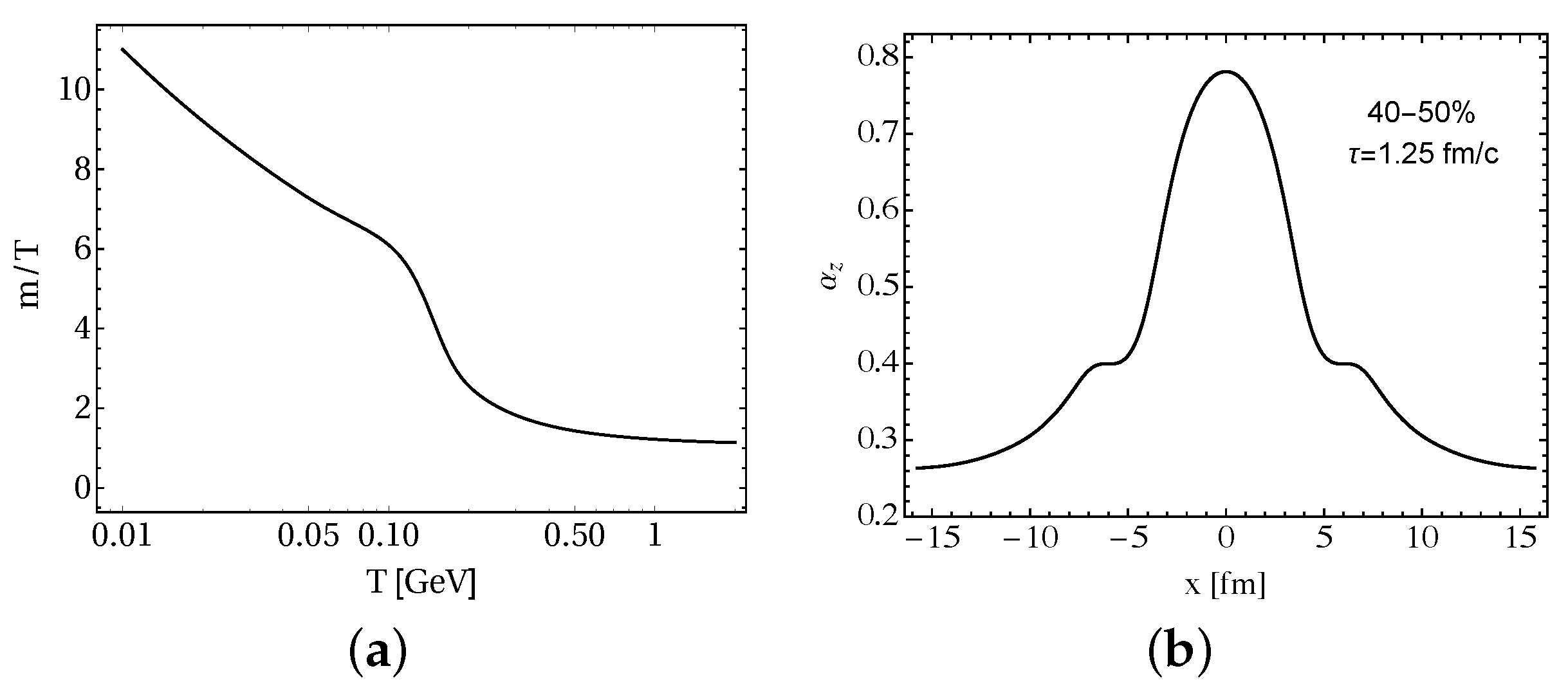
5. Evolution and Freezeout in aHydroQP

The evolution equations for u μ , λ , and α i are obtained from moments of the quasiparticle Boltzmann equation. These can be expressed compactly by introducing a timelike vector u μ which is normalized as u μ u μ = 1 and three spacelike vectors X i μ which are individually normalized as X i μ X μ , i = 1 . These vectors are mutually orthogonal and obey u μ X i μ and X μ , i X j μ = 0 for i j [48,50]. The four equations resulting from the first moment are
D u ϵ + ϵ θ u + j P j u μ D j X j μ = 0 ,
D i P i + P i θ i ϵ X μ , i D u u μ + P i X μ , i D i X i μ j P j X μ , i D j X j μ = 0 ,
where i , j { x , y , z } , D u u μ μ , and D i X i μ μ . The expansion scalars are θ u = μ u μ and θ i = μ X i μ . Explicit expressions for the basis vectors, derivative operators and expansion scalars can be found in Refs. [18,54,60,64]. The quantities ϵ and P i are the kinetic energy density and pressures obtained using the anisotropic hydrodynamics ansatz for the one-particle distributions function corrected by the background contribution B ( T ) necessary to enforce thermodynamic consistency
ϵ = ϵ kinetic ( λ , α , m ) + B ( λ , α ) ,
P i = P i , kinetic ( λ , α , m ) B ( λ , α ) ,
The three equations resulting from the second moment of the Boltzmann equation are
D u I i + I i ( θ u + 2 u μ D i X i μ ) = 1 τ eq I eq ( T , m ) I i ,
with [54]
I i = α α i 2 I eq ( λ , m ) , I eq ( λ , m ) = 4 π N ˜ λ 5 m ^ 3 K 3 ( m ^ ) ,
where m ^ = m / λ , α = α x α y α z and N ˜ = N dof / ( 2 π ) 3 , with N dof being the number of degrees of freedom present in the theory under consideration.
Equations (30), (31) and (34) provide seven partial differential equations for u , α , and λ which we solve numerically. For this purpose, we use fourth-order Runga-Kutta integration of the equations of motion in time and a weighted-LAX scheme to regulate shock propagation. For details of the numerical algorithm, we refer the reader to Ref. [50].
To determine the local effective temperature we make use of Landau matching; requiring the equilibrium and non-equilibrium energy densities in the LRF to be equal and solving for T. Herein, we assume the system to initially be isotropic in momentum space α i ( τ 0 ) = 1 , with zero transverse flow. However, the system evolves quite fast away from isotropy τ aniso 1 fm. As an example, in Figure 1-right panel we show the spatial profile of the longitudinal anisotropy parameter at 40–50% centrality class. As can be seen from this figure, α z differs from unity especially in the dilute regions | x | > 5 fm. We note here that no regulation is required in aHydroQP to evolve in these dilute regions. This system of partial differential equations keep evolving until the effective temperature in the entire simulation volume falls below a given freeze-out temperature of T FO . From the results, we extract a three-dimensional freeze-out hypersurface with a fixed energy density (temperature). We assume in this step that the fluid anisotropy tensor and scale parameter are the same for all hadronic species. We also assume that all hadrons created are in chemical equilibrium. With the use of an extended Cooper-Frye prescription [76], we are able to translate the underlying hydrodynamic evolution values for the flow velocity, the anisotropy parameters, and the scale into explicit ’primordial’ hadronic distribution functions on this hypersurface.
The values of the aHydroQP parameters on the freezeout hypersurface are passed to a modified version of THERMINATOR 2 [79], which generates hadronic configurations using Monte-Carlo sampling. The modification consisted of changing the underlying assumption for the one-particle distribution function from the canonical linearized viscous hydrodynamics form to the aHydroQP form including three anisotropy parameters in the local rest frame. After sampling the primordial hadrons, further hadronic decays are taken into account using the built-in routines in THERMINATOR 2. The source code for aHydroQP and our custom version of THERMINATOR 2 are both freely accessible [80]. The aHydroQP formalism was used at different collision energies, and it was found that the observed differential spectra of identified hadrons, charged particle multiplicity, elliptic flow, and Hanbury-Brown-Twiss radii could be reproduced.
Finally, in Table 1 we list the fitting parameters that we extracted and used in the comparisons.

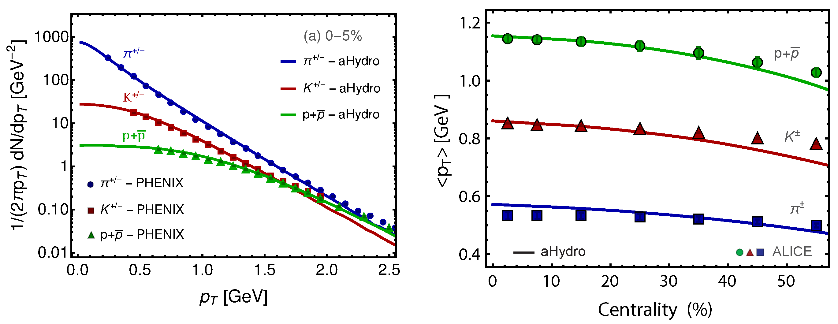
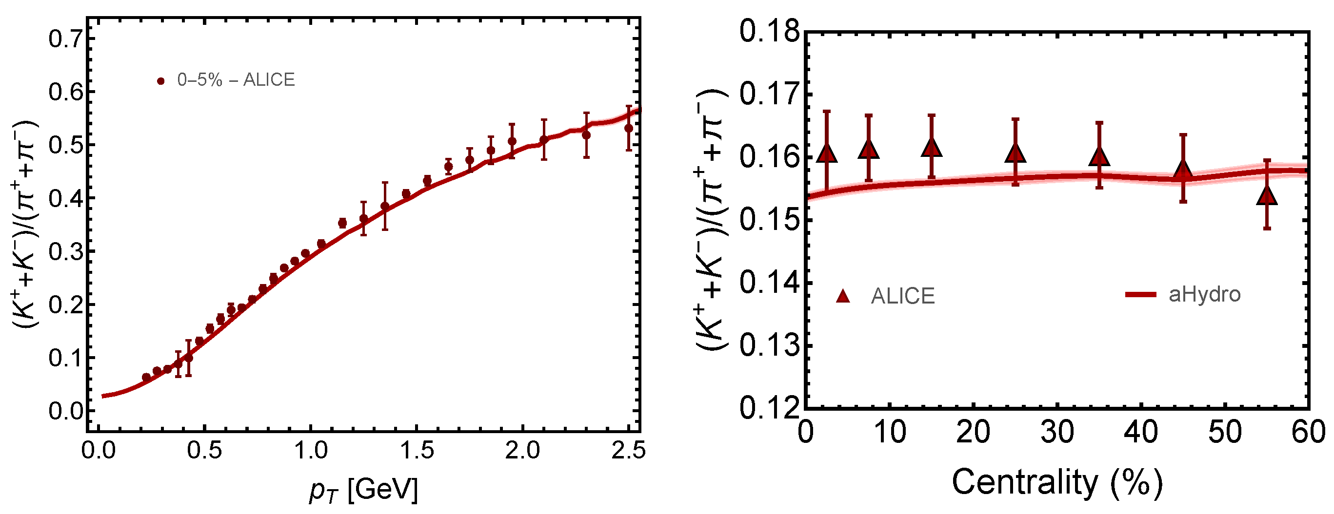
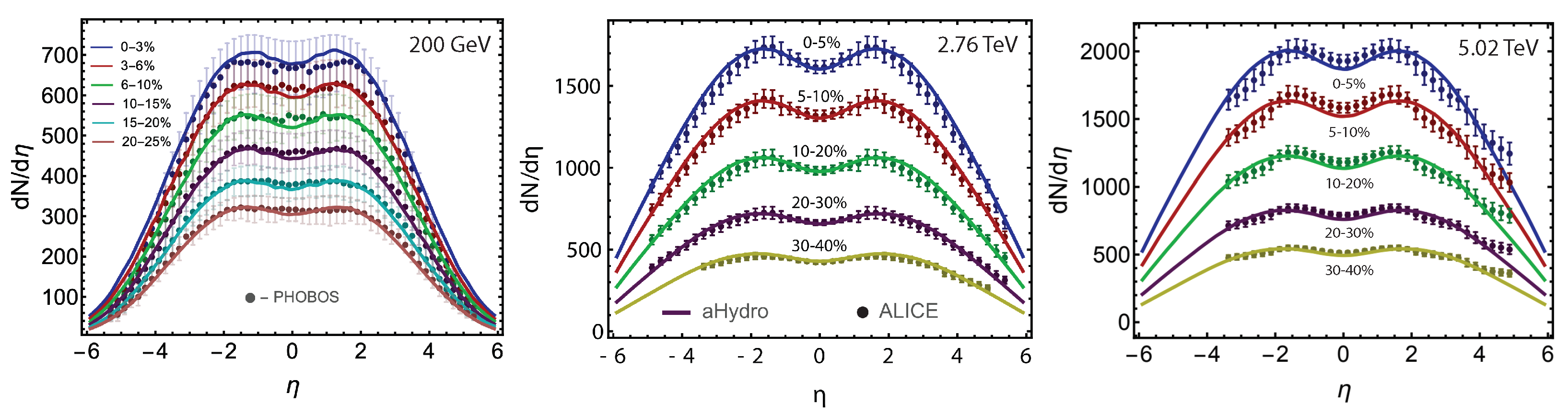
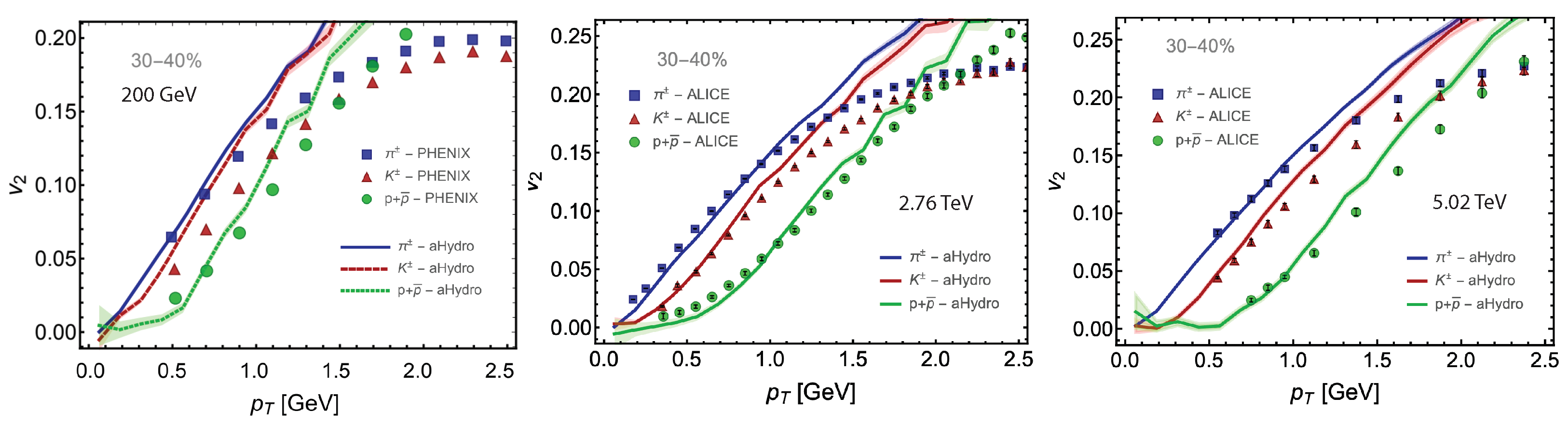
6. Results and Discussion

In this section, we present phenomenological comparisons of 3+1D aHydroQP model to experimental data. For the sake of brevity, we present comparisons of a small set of observables performed at various collision energies s N N = 200 GeV, 2.76, 5.02 TeV for Au-Au and Pb-Pb collisions from the PHENIX, PHOBOS, STAR, and ALICE collaborations.
We first present comparisons of bulk observables between our model and experimental results. In Figure 2, (left panel), we show the spectra of pions, kaons, and protons as a function of the transverse momentum p T . The agreement shown between our model and the experimental results is good up to quite large p T 2 GeV. In this figure, we show only one centrality class 0–5%, however one can see Ref. [82] for more comparisons up to 30–40% centrality class. It suffices here to say that the agreement is quite good up to p T 1.5 GeV for high centrality classes. Next, we present the centrality dependence of the average transverse momentum of pions, kaons, and protons at 2.76 TeV in Pb-Pb collisions. Again, the agreement is very good up to high centrality classes ∼50%. The spectra at this energy is not presented here, however, it can be found in Ref. [64], where the agreement between aHydroQP model and the data for different centrality classes is good.
Next, in the left panel of Figure 3, the kaon-to-pion yield ratio ( K + + K ) / ( π + + π ) is presented as a function of p T in the 0–5% centrality class. As can be seen from this figure, our model was able to reproduce the ratios well up to fairly large p T 2.5 GeV. We also show, in Figure 3-right panel, the kaon-to-pion yield ratio as a function of centrality where our model again describes the data quite well over a wide range of centrality classes. In ref. [78], we showed the kaon-to-pion ratio ratio and also the proton-to-pion yield ratio for multiple different centrality classes with a reasonable agreement to the data at 5.023 TeV for Pb-Pb collisions from ALICE collaboration.
Next, we present, in Figure 4, the charged particle multiplicity as a function of the pseduorapidity where data are from the PHOBOS and ALICE collaborations for Au+Au and Pb-Pb collisions, respectively. In the left panel, the multiplicity is shown for 0–3%, 3–6%, 6–10%, 10–15%, 15–20%, and 20–25% centrality classes. Whereas in the middle and right panels, the multiplicity is shown for 0–5%, 5–10%, 10–20%, 20–30%, and 30–40% centrality classes. We find that our model does a good job in reproducing the pseudorapidity dependence of the multiplicity in a wide range of centrality classes.
Furthermore, in Figure 5 we present comparisons of the anisotropic flow, in the 30–40% centrality class, where data are from the PHENIX and ALICE collaborations for Au+Au and Pb-Pb collisions, respectively. As can be seen from all three panels, our model shows reasonable agreement with data at low p T . A similar agreement between this model and experimental data is seen across different centrality classes, see Refs. [64,78,82].
Finally, we present the aHydroQP predictions for HBT radii determined from pion correlations. As an example, in Figure 6, we show the R o u t / R s i d e ratio as a function of the mean transverse momentum of the pair π + π + in the 5–10 % centrality class. As can be seen from this figure, our model was able to describe the experimental data from the STAR collaboration quite well especially for low k T up to 0.4 GeV. For more details, see [91]. We not here that a similar agreement of the HBT radii and thier ratios to the data is seen at 2.76 TeV for Pb-Pb collisions [64].

7. Conclusions

In this review we presented a summary of recent progress in anisotropic hydrodynamics and its application to heavy-ion phenomenology. We began with a demonstration in the simple case of conformal Bjorken expansion that aHydro resums an infinite number of terms in the inverse Reynolds number. This feature allows aHydro to better describe systems that are far from equilibrium than traditional approaches. In AA collision large non-equilibrium corrections occur during the initial stages of the QGP ( τ < 1 fm/c) and at all times near the cold edges of the plasma where the relaxation time grows large. In collisions of small systems such as pA and pp one expects that, if a QGP is generated, it will be much more short-lived than in central AA collisions due to larger transverse gradients and, as a consequence, it will experience larger deviations from equilibrium during its evolution and freeze out.
Turning to AA phenomenology, we presented comparisons between the 3+1D aHydroQP model and heavy-ion experimental data collected at RHIC and LHC. We list the extracted initial central temperature and shear viscosity at 200 GeV, 2.76 TeV, and 5.02 TeV in Table 1. At all three collision energies with these parameters, we were able to describe the identified hadron spectra well, including the p T -dependence of the kaon-to-pion yield ratio. In addition, the extracted integrated elliptic flow for charged particles and p T -dependence of the pion, proton, and kaon elliptic flow were found to also be in good agreement with the data. Finally, we also presented comparisons between aHydroQP model predictions and STAR data from the ratio of ‘out’ and ‘side’ HBT radii, again finding good agreement with the data given current experimental uncertainties.
Looking to the future, final work is underway to release a new computational pipeline for 3+1D aHydroQP which includes fluctuating initial conditions of various types such as Trento [93,94] or IP-Glasma [95,96,97], a custom anisotropic hadronic freeze-out sampler based on ISS [98], and full URQMD [99,100] or SMASH [101] hadronic afterburners that include elastic as well as inelastic channels. Once complete, this will allow us to compute higher-order flow coefficients using aHydroQP in AA, pA, and pp collisions.

Author Contributions

H.A., M.A. and M.S. contributed equally to writing this review. All authors have read and agreed to the published version of the manuscript.

Funding

H. Alalawi was supported by a visiting Ph.D. scholarship from Umm Al-Qura University. M. Alqahtani was supported by the Deanship of Scientific Research at the Imam Abdulrahman Bin Faisal University under grant number 2021-089-CED. M. Strickland was supported by the U.S. Department of Energy, Office of Science, Office of Nuclear Physics under Award No. DE-SC0013470.

Institutional Review Board Statement

Not applicable.

Informed Consent Statement

Not applicable.

Data Availability Statement

The code necessary to generate all results shown can be downloaded from https://www.personal.kent.edu/~mstrick6/code/index.html.

Conflicts of Interest

The authors declare no conflict of interest.

References

  1. Averbeck, R.; Harris, J.W.; Schenke, B. Heavy-Ion Physics at the LHC. In The Large Hadron Collider: Harvest of Run 1; Schörner-Sadenius, T., Ed.; Springer International Publishing: Cham, Switzerland, 2015; pp. 355–420. [Google Scholar]
  2. Wang, X.N. (Ed.) Quark-Gluon Plasma 5; World Scientific: Singapore, 2016. [Google Scholar]
  3. Dexheimer, V.; Noronha, J.; Noronha-Hostler, J.; Ratti, C.; Yunes, N. Future physics perspectives on the equation of state from heavy ion collisions to neutron stars. J. Phys. G 2021, 48, 073001. [Google Scholar] [CrossRef]
  4. Bazavov, A. An overview of (selected) recent results in finite-temperature lattice QCD. J. Phys. Conf. Ser. 2013, 446, 012011. [Google Scholar] [CrossRef] [Green Version]
  5. Borsanyi, S. Frontiers of finite temperature lattice QCD. EPJ Web Conf. 2017, 137, 01006. [Google Scholar] [CrossRef] [Green Version]
  6. Cea, P.; Cosmai, L.; Papa, A. Critical line of 2+1 flavor QCD: Toward the continuum limit. Phys. Rev. D 2016, 93, 014507. [Google Scholar] [CrossRef] [Green Version]
  7. Bonati, C.; D’Elia, M.; Mariti, M.; Mesiti, M.; Negro, F.; Sanfilippo, F. Curvature of the chiral pseudocritical line in QCD: Continuum extrapolated results. Phys. Rev. D 2015, 92, 054503. [Google Scholar] [CrossRef] [Green Version]
  8. Bonati, C.; D’Elia, M.; Negro, F.; Sanfilippo, F.; Zambello, K. Curvature of the pseudocritical line in QCD: Taylor expansion matches analytic continuation. Phys. Rev. D 2018, 98, 054510. [Google Scholar] [CrossRef] [Green Version]
  9. Bonati, C.; D’Elia, M.; Mariti, M.; Mesiti, M.; Negro, F.; Sanfilippo, F. Curvature of the chiral pseudocritical line in QCD. Phys. Rev. D 2014, 90, 114025. [Google Scholar] [CrossRef] [Green Version]
  10. Borsanyi, S.; Fodor, Z.; Guenther, J.N.; Kara, R.; Katz, S.D.; Parotto, P.; Pasztor, A.; Ratti, C.; Szabo, K.K. QCD Crossover at Finite Chemical Potential from Lattice Simulations. Phys. Rev. Lett. 2020, 125, 052001. [Google Scholar] [CrossRef]
  11. Bazavov, A.; Ding, H.T.; Hegde, P.; Kaczmarek, O.; Karsch, F.; Karthik, N.; Laermann, E.; Lahiri, A.; Larsen, R.; Li, S.T.; et al. Chiral crossover in QCD at zero and non-zero chemical potentials. Phys. Lett. B 2019, 795, 15–21. [Google Scholar] [CrossRef]
  12. Toublan, D.; Kogut, J.B. The QCD phase diagram at nonzero baryon, isospin and strangeness chemical potentials: Results from a hadron resonance gas model. Phys. Lett. B 2005, 605, 129–136. [Google Scholar] [CrossRef] [Green Version]
  13. Endrodi, G.; Fodor, Z.; Katz, S.D.; Szabo, K.K. The QCD phase diagram at nonzero quark density. J. High Energy Phys. 2011, 4, 1–4. [Google Scholar] [CrossRef] [Green Version]
  14. Bellwied, R.; Borsanyi, S.; Fodor, Z.; Günther, J.; Katz, S.D.; Ratti, C.; Szabo, K.K. The QCD phase diagram from analytic continuation. Phys. Lett. B 2015, 751, 559–564. [Google Scholar] [CrossRef] [Green Version]
  15. Berges, J.; Borsányi, S. Range of validity of transport equations. Phys. Rev. D 2006, 74, 045022. [Google Scholar] [CrossRef] [Green Version]
  16. Haque, N.; Strickland, M. Next-to-next-to leading-order hard-thermal-loop perturbation-theory predictions for the curvature of the QCD phase transition line. Phys. Rev. C 2021, 103, 031901. [Google Scholar] [CrossRef]
  17. Huovinen, P.; Petreczky, P. QCD Equation of State and Hadron Resonance Gas. Nucl. Phys. A 2010, 837, 26–53. [Google Scholar] [CrossRef] [Green Version]
  18. Alqahtani, M.; Nopoush, M.; Strickland, M. Quasiparticle equation of state for anisotropic hydrodynamics. Phys. Rev. C 2015, 92, 54910. [Google Scholar] [CrossRef] [Green Version]
  19. Parotto, P.; Bluhm, M.; Mroczek, D.; Nahrgang, M.; Noronha-Hostler, J.; Rajagopal, K.; Ratti, C.; Schäfer, T.; Stephanov, M. QCD equation of state matched to lattice data and exhibiting a critical point singularity. Phys. Rev. C 2020, 101, 34901. [Google Scholar] [CrossRef] [Green Version]
  20. Jeon, S.; Heinz, U. Introduction to Hydrodynamics. In Quark-Gluon Plasma 5; Wang, X.N., Ed.; World Scientific: Singapore, 2016; pp. 131–187. [Google Scholar]
  21. Borsányi, S.; Endrődi, G.; Fodor, Z.; Jakovác, A.; Katz, S.D.; Krieg, S.; Ratti, C.; Szabó, K.K. The QCD equation of state with dynamical quarks. J. High Energy Phys. 2010, 2010, 1–33. [Google Scholar] [CrossRef] [Green Version]
  22. Romatschke, P.; Romatschke, U. Relativistic Fluid Dynamics in and out of Equilibrium; Cambridge Monographs on Mathematical Physics, Cambridge University Press: Cambridge, UK, 2019. [Google Scholar]
  23. Huovinen, P.; Kolb, P.; Heinz, U.; Ruuskanen, P.; Voloshin, S. Radial and elliptic flow at RHIC: Further predictions. Phys. Lett. B 2001, 503, 58–64. [Google Scholar] [CrossRef] [Green Version]
  24. Hirano, T.; Tsuda, K. Collective flow and two pion correlations from a relativistic hydrodynamic model with early chemical freeze out. Phys. Rev. 2002, 66, 054905. [Google Scholar] [CrossRef] [Green Version]
  25. Kolb, P.F.; Heinz, U.W. Hydrodynamic description of ultrarelativistic heavy ion collisions. In Quark-Gluon Plasma 3; World Scientific: Singapore, 2003; pp. 634–714. [Google Scholar]
  26. Danielewicz, P.; Gyulassy, M. Dissipative Phenomena in Quark Gluon Plasmas. Phys. Rev. D 1985, 31, 53–62. [Google Scholar] [CrossRef] [PubMed] [Green Version]
  27. Policastro, G.; Son, D.T.; Starinets, A.O. The Shear viscosity of strongly coupled N=4 supersymmetric Yang–Mills plasma. Phys. Rev. Lett. 2001, 87, 081601. [Google Scholar] [CrossRef] [PubMed] [Green Version]
  28. Muronga, A. Second order dissipative fluid dynamics for ultrarelativistic nuclear collisions. Phys. Rev. Lett. 2002, 88, 062302, Erratum in Phys. Rev. Lett. 2002, 89, 159901. [Google Scholar] [CrossRef] [PubMed] [Green Version]
  29. Muronga, A. Causal theories of dissipative relativistic fluid dynamics for nuclear collisions. Phys. Rev. C 2004, 69, 034903. [Google Scholar] [CrossRef] [Green Version]
  30. Muronga, A.; Rischke, D.H. Evolution of hot, dissipative quark matter in relativistic nuclear collisions. arXiv 2004, arXiv:nucl-th/0407114. [Google Scholar]
  31. Heinz, U.W.; Song, H.; Chaudhuri, A.K. Dissipative hydrodynamics for viscous relativistic fluids. Phys. Rev. C 2006, 73, 034904. [Google Scholar] [CrossRef] [Green Version]
  32. Baier, R.; Romatschke, P.; Wiedemann, U.A. Dissipative hydrodynamics and heavy ion collisions. Phys. Rev. C 2006, 73, 064903. [Google Scholar] [CrossRef] [Green Version]
  33. Romatschke, P.; Romatschke, U. Viscosity Information from Relativistic Nuclear Collisions: How Perfect is the Fluid Observed at RHIC? Phys. Rev. Lett. 2007, 99, 172301. [Google Scholar] [CrossRef] [Green Version]
  34. Baier, R.; Romatschke, P.; Son, D.T.; Starinets, A.O.; Stephanov, M.A. Relativistic viscous hydrodynamics, conformal invariance, and holography. J. High Energy Phys. 2008, 4, 100. [Google Scholar] [CrossRef]
  35. Denicol, G.S.; Niemi, H.; Molnar, E.; Rischke, D.H. Derivation of transient relativistic fluid dynamics from the Boltzmann equation. Phys. Rev. D 2015, 85, 114047, Erratum in Phys. Rev. D 2015, 91, 039902. [Google Scholar] [CrossRef] [Green Version]
  36. Denicol, G.S.; Molnár, E.; Niemi, H.; Rischke, D.H. Derivation of fluid dynamics from kinetic theory with the 14-moment approximation. Eur. Phys. J. A 2012, 48, 170. [Google Scholar] [CrossRef] [Green Version]
  37. Jaiswal, A. Relativistic dissipative hydrodynamics from kinetic theory with relaxation time approximation. Phys. Rev. C 2013, 87, 051901. [Google Scholar] [CrossRef]
  38. Jaiswal, A. Relativistic third-order dissipative fluid dynamics from kinetic theory. Phys. Rev. C 2013, 88, 021903. [Google Scholar] [CrossRef] [Green Version]
  39. Calzetta, E. Hydrodynamic approach to boost invariant free streaming. Phys. Rev. D 2015, 92, 045035. [Google Scholar] [CrossRef] [Green Version]
  40. Denicol, G.S.; Jeon, S.; Gale, C. Transport Coefficients of Bulk Viscous Pressure in the 14-moment approximation. Phys. Rev. C 2014, 90, 024912. [Google Scholar] [CrossRef] [Green Version]
  41. Denicol, G.S.; Florkowski, W.; Ryblewski, R.; Strickland, M. Shear-bulk coupling in nonconformal hydrodynamics. Phys. Rev. C 2014, 90, 044905. [Google Scholar] [CrossRef] [Green Version]
  42. Jaiswal, A.; Ryblewski, R.; Strickland, M. Transport coefficients for bulk viscous evolution in the relaxation time approximation. Phys. Rev. C 2014, 90, 044908. [Google Scholar] [CrossRef] [Green Version]
  43. Bemfica, F.S.; Disconzi, M.M.; Noronha, J. General-Relativistic Viscous Fluid Dynamics. arXiv 2020, arXiv:2009.11388. [Google Scholar]
  44. Hoult, R.E.; Kovtun, P. Stable and causal relativistic Navier–Stokes equations. J. High Energy Phys. 2020, 6, 1–5. [Google Scholar] [CrossRef]
  45. Heinz, U.W.; Bazow, D.; Strickland, M. Viscous hydrodynamics for strongly anisotropic expansion. Nucl. Phys. A 2014, 931, 920–925. [Google Scholar] [CrossRef] [Green Version]
  46. Florkowski, W.; Ryblewski, R. Highly-anisotropic and strongly-dissipative hydrodynamics for early stages of relativistic heavy-ion collisions. Phys. Rev. C 2011, 83, 034907. [Google Scholar] [CrossRef]
  47. Martinez, M.; Strickland, M. Dissipative Dynamics of Highly Anisotropic Systems. Nucl. Phys. A 2010, 848, 183–197. [Google Scholar] [CrossRef] [Green Version]
  48. Ryblewski, R.; Florkowski, W. Highly anisotropic hydrodynamics – discussion of the model assumptions and forms of the initial conditions. Acta Phys. Polon. B 2011, 42, 115–138. [Google Scholar] [CrossRef]
  49. Florkowski, W.; Ryblewski, R. Projection method for boost-invariant and cylindrically symmetric dissipative hydrodynamics. Phys. Rev. C 2012, 85, 044902. [Google Scholar] [CrossRef] [Green Version]
  50. Martinez, M.; Ryblewski, R.; Strickland, M. Boost-Invariant (2+1)-dimensional Anisotropic Hydrodynamics. Phys. Rev. C 2012, 85, 064913. [Google Scholar] [CrossRef] [Green Version]
  51. Ryblewski, R.; Florkowski, W. Highly-anisotropic hydrodynamics in 3+1 space-time dimensions. Phys. Rev. C 2012, 85, 064901. [Google Scholar] [CrossRef] [Green Version]
  52. Bazow, D.; Heinz, U.W.; Strickland, M. Second-order (2+1)-dimensional anisotropic hydrodynamics. Phys. Rev. C 2014, 90, 054910. [Google Scholar] [CrossRef] [Green Version]
  53. Tinti, L.; Florkowski, W. Projection method and new formulation of leading-order anisotropic hydrodynamics. Phys. Rev. C 2014, 89, 034907. [Google Scholar] [CrossRef] [Green Version]
  54. Nopoush, M.; Ryblewski, R.; Strickland, M. Bulk viscous evolution within anisotropic hydrodynamics. Phys. Rev. C 2014, 90, 014908. [Google Scholar] [CrossRef] [Green Version]
  55. Tinti, L. Anisotropic matching principle for the hydrodynamic expansion. Phys. Rev. C 2016, 94, 044902. [Google Scholar] [CrossRef] [Green Version]
  56. Bazow, D.; Heinz, U.W.; Martinez, M. Nonconformal viscous anisotropic hydrodynamics. Phys. Rev. C 2015, 91, 064903. [Google Scholar] [CrossRef] [Green Version]
  57. Strickland, M.; Nopoush, M.; Ryblewski, R. Anisotropic hydrodynamics for conformal Gubser flow. Nucl. Phys. A 2016, 956, 268–271. [Google Scholar] [CrossRef] [Green Version]
  58. Molnar, E.; Niemi, H.; Rischke, D.H. Derivation of anisotropic dissipative fluid dynamics from the Boltzmann equation. Phys. Rev. D 2016, 93, 114025. [Google Scholar] [CrossRef] [Green Version]
  59. Molnár, E.; Niemi, H.; Rischke, D.H. Closing the equations of motion of anisotropic fluid dynamics by a judicious choice of a moment of the Boltzmann equation. Phys. Rev. D 2016, 94, 125003. [Google Scholar] [CrossRef] [Green Version]
  60. Alqahtani, M.; Nopoush, M.; Strickland, M. Quasiparticle anisotropic hydrodynamics for central collisions. Phys. Rev. C 2017, 95, 034906. [Google Scholar] [CrossRef]
  61. Bluhm, M.; Schäfer, T. Dissipative fluid dynamics for the dilute Fermi gas at unitarity: Anisotropic fluid dynamics. Phys. Rev. A 2015, 92, 043602. [Google Scholar] [CrossRef] [Green Version]
  62. Bluhm, M.; Schaefer, T. Model-independent determination of the shear viscosity of a trapped unitary Fermi gas: Application to high temperature data. Phys. Rev. Lett. 2016, 116, 115301. [Google Scholar] [CrossRef] [Green Version]
  63. Alqahtani, M.; Nopoush, M.; Ryblewski, R.; Strickland, M. (3+1)D Quasiparticle Anisotropic Hydrodynamics for Ultrarelativistic Heavy-Ion Collisions. Phys. Rev. Lett. 2017, 119, 042301. [Google Scholar] [CrossRef] [Green Version]
  64. Alqahtani, M.; Nopoush, M.; Ryblewski, R.; Strickland, M. Anisotropic hydrodynamic modeling of 2.76 TeV Pb-Pb collisions. Phys. Rev. C 2017, 96, 044910. [Google Scholar] [CrossRef] [Green Version]
  65. Almaalol, D.; Alqahtani, M.; Strickland, M. Anisotropic hydrodynamics with number-conserving kernels. Phys. Rev. C 2019, 99, 014903. [Google Scholar] [CrossRef] [Green Version]
  66. Almaalol, D.; Strickland, M. Anisotropic hydrodynamics with a scalar collisional kernel. Phys. Rev. C 2018, 97, 044911. [Google Scholar] [CrossRef] [Green Version]
  67. McNelis, M.; Bazow, D.; Heinz, U. (3+1)-dimensional anisotropic fluid dynamics with a lattice QCD equation of state. Phys. Rev. C 2018, 97, 054912. [Google Scholar] [CrossRef] [Green Version]
  68. Nopoush, M.; Strickland, M. Including off-diagonal anisotropies in anisotropic hydrodynamics. Phys. Rev. C 2019, 100, 014904. [Google Scholar] [CrossRef] [Green Version]
  69. Słodkowski, M.; Setniewski, D.; Aszklar, P.; Porter-Sobieraj, J. Modeling the Dynamics of Heavy-Ion Collisions with a Hydrodynamic Model Using a Graphics Processor. Symmetry 2021, 13, 507. [Google Scholar] [CrossRef]
  70. McNelis, M.; Bazow, D.; Heinz, U. Anisotropic fluid dynamical simulations of heavy-ion collisions. Comput. Phys. Commun. 2021, 267, 108077. [Google Scholar] [CrossRef]
  71. Romatschke, P.; Strickland, M. Collective modes of an anisotropic quark gluon plasma. Phys. Rev. D 2003, 68, 036004. [Google Scholar] [CrossRef] [Green Version]
  72. Strickland, M.; Noronha, J.; Denicol, G. Anisotropic nonequilibrium hydrodynamic attractor. Phys. Rev. D 2018, 97, 036020. [Google Scholar] [CrossRef] [Green Version]
  73. Martinez, M.; McNelis, M.; Heinz, U. Anisotropic fluid dynamics for Gubser flow. Phys. Rev. C 2017, 95, 054907. [Google Scholar] [CrossRef] [Green Version]
  74. Denicol, G.S.; Koide, T.; Rischke, D.H. Dissipative relativistic fluid dynamics: A new way to derive the equations of motion from kinetic theory. Phys. Rev. Lett. 2010, 105, 162501. [Google Scholar] [CrossRef]
  75. Denicol, G.S. Kinetic foundations of relativistic dissipative fluid dynamics. J. Phys. G 2014, 41, 124004. [Google Scholar] [CrossRef]
  76. Alqahtani, M.; Nopoush, M.; Strickland, M. Relativistic anisotropic hydrodynamics. Prog. Part. Nucl. Phys. 2018, 101, 204–248. [Google Scholar] [CrossRef] [Green Version]
  77. Ryblewski, R. Thermodynamically consistent formulation of quasiparticle viscous hydrodynamics. Acta Phys. Polon. Suppl. 2017, 10, 1073. [Google Scholar] [CrossRef] [Green Version]
  78. Alqahtani, M.; Strickland, M. Bulk observables at 5.02 TeV using quasiparticle anisotropic hydrodynamics. Eur. Phys. J. C 2021, 81, 1022. [Google Scholar] [CrossRef]
  79. Chojnacki, M.; Kisiel, A.; Florkowski, W.; Broniowski, W. THERMINATOR 2: THERMal heavy IoN generATOR 2. Comput. Phys. Commun. 2012, 183, 746–773. [Google Scholar] [CrossRef] [Green Version]
  80. Alqahtani, M.; Nopoush, M.; Ryblewski, R.; Strickland, M. KSU Code Repo. 2021. Available online: http://personal.kent.edu/~mstrick6/code (accessed on 28 December 2021).
  81. Adler, S.S.; Afanasiev, S.; Aidala, C.; Ajitanand, N.N.; Akiba, Y.; Alexander, J.; Amirikas, R.; Aphecetche, L.; Aronson, S.H.; Averbeck, R.; et al. Identified charged particle spectra and yields in Au+Au collisions at S(NN)**1/2 = 200-GeV. Phys. Rev. C 2004, 69, 034909. [Google Scholar] [CrossRef] [Green Version]
  82. Almaalol, D.; Alqahtani, M.; Strickland, M. Anisotropic hydrodynamic modeling of 200 GeV Au-Au collisions. Phys. Rev. C 2019, 99, 044902. [Google Scholar] [CrossRef] [Green Version]
  83. Abelev, B.; ALICE Collaboration. Centrality dependence of π, K, p production in Pb-Pb collisions at s N N = 2.76 TeV. Phys. Rev. C 2013, 88, 044910. [Google Scholar] [CrossRef] [Green Version]
  84. Acharya, S.; Adamová, D.; Adhya, S.P.; Adler, A.; Adolfsson, J.; Aggarwal, M.M.; Rinella, G.A.; Agnello, M.; Agrawal, N.; Ahammed, Z.; et al. Production of charged pions, kaons, and (anti-)protons in Pb-Pb and inelastic pp collisions at s N N = 5.02 TeV. Phys. Rev. C 2020, 101, 044907. [Google Scholar] [CrossRef]
  85. Alver, B.; Back, B.B.; Baker, M.D.; Ballintijn, M.; Barton, D.S.; Betts, R.R.; Bickley, A.A.; Bindel, R.; Budzanowski, A.; Busza, W.; et al. Phobos results on charged particle multiplicity and pseudorapidity distributions in Au+Au, Cu+Cu, d+Au, and p+p collisions at ultra-relativistic energies. Phys. Rev. C 2011, 83, 024913. [Google Scholar] [CrossRef] [Green Version]
  86. Adam, J.; Adamova, D.; Aggarwal, M.M.; Rinella, G.A.; Agnello, M.; Agrawal, N.; Ahammed, Z.; Ahn, S.U.; Aiola, S.; Akindinov, A.; et al. Centrality evolution of the charged-particle pseudorapidity density over a broad pseudorapidity range in Pb-Pb collisions at s N N = 2.76 TeV. Phys. Lett. B 2016, 754, 373–385. [Google Scholar] [CrossRef]
  87. Adam, J.; Aggarwal, M.M.; Aglieri Rinella, G.; Agrawal, N.; Ahammed, Z.; Ahmad, S.F.; Ahn, S.U.; Aimo, I.; Akindinov, A.; Alam, S.N.; et al. Centrality dependence of the pseudorapidity density distribution for charged particles in Pb-Pb collisions at s N N =5.02 TeV. Phys. Lett. B 2017, 772, 567–577. [Google Scholar] [CrossRef] [Green Version]
  88. Adare, A.; Afanasiev, S.; Aidala, C.; Ajitanand, N.N.; Akiba, Y.; Al-Bataineh, H.; Alexander, J.; Aoki, K.; Aramaki, Y.; Atomssa, E.T.; et al. Measurement of the higher-order anisotropic flow coefficients for identified hadrons in Au+Au collisions at s N N = 200 GeV. Phys. Rev. C 2016, 93, 051902. [Google Scholar] [CrossRef] [Green Version]
  89. Abelev, B.B.; Adam, J.; Adamová, D.; Aggarwal, M.M.; Agnello, M.; Agostinelli, A.; Agrawal, N.; Ahammed, Z.; Ahmad, N.; Ahmed, I.; et al. Elliptic flow of identified hadrons in Pb-Pb collisions at s N N =2.76 TeV. J. High Energy Phys. 2015, 6, 190. [Google Scholar] [CrossRef]
  90. Acharya, S.; Adamová, D.; Adolfsson, J.; Aggarwal, M.M.; Rinella, G.A.; Agnello, M.; Agrawal, N.; Ahammed, Z.; Ahn, S.U.; Aiola, S.; et al. Anisotropic flow of identified particles in Pb-Pb collisions at s N N =5.02 TeV. J. High Energy Phys. 2018, 9, 6. [Google Scholar]
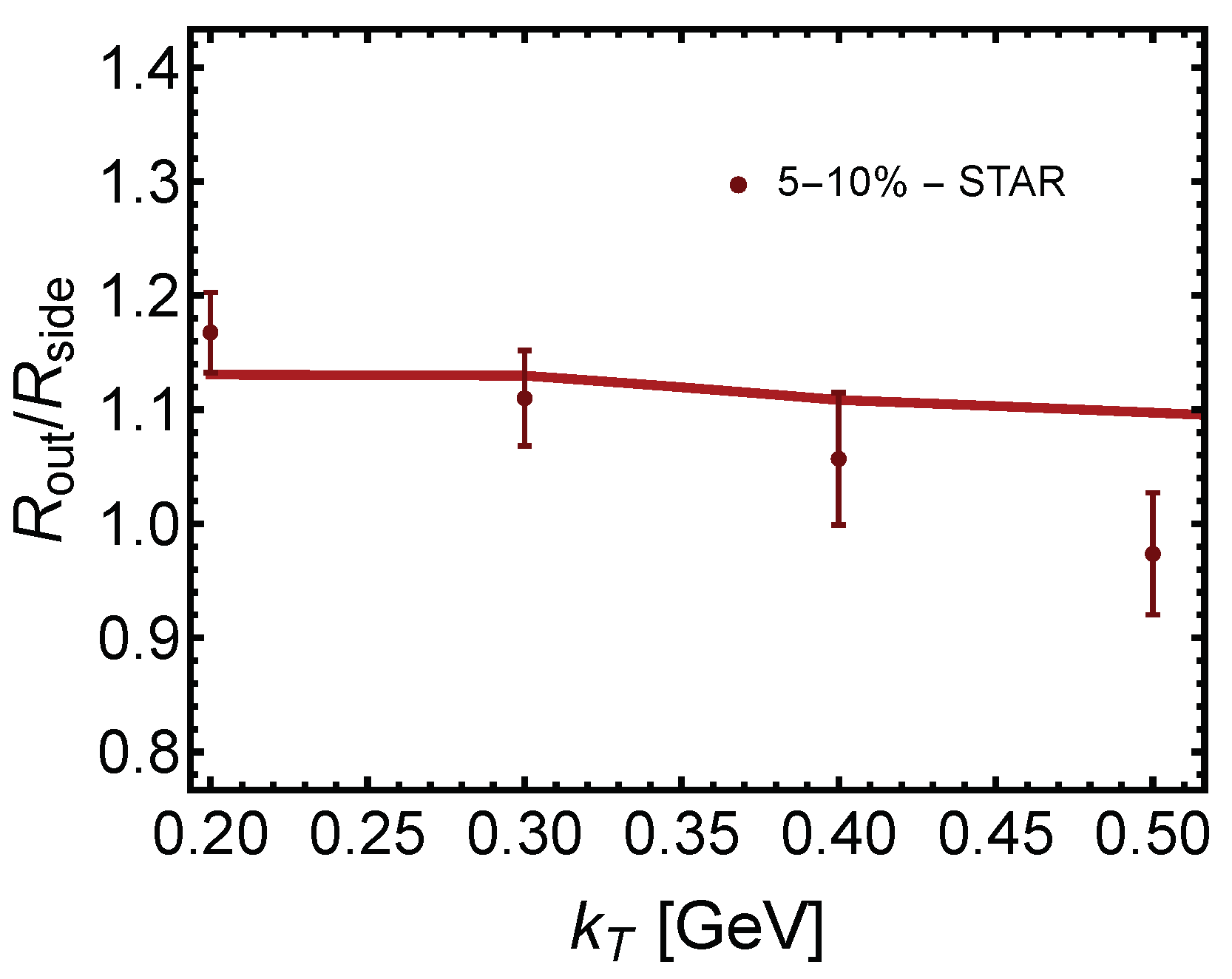
  91. Alqahtani, M.; Strickland, M. Pion interferometry at 200 GeV using anisotropic hydrodynamics. Phys. Rev. C 2020, 102, 064902. [Google Scholar] [CrossRef]
  92. Adams, J.; Aggarwal, M.M.; Ahammed, Z.; Amonett, J.; Anderson, B.D.; Arkhipkin, D.; Averichev, G.S.; Badyal, S.K.; Bai, Y.; Balewski, J.; et al. Pion interferometry in Au+Au collisions at S(NN)**(1/2) = 200-GeV. Phys. Rev. C 2005, 71, 044906. [Google Scholar] [CrossRef] [Green Version]
  93. Moreland, J.S.; Bernhard, J.E.; Bass, S.A. Alternative ansatz to wounded nucleon and binary collision scaling in high-energy nuclear collisions. Phys. Rev. C 2015, 92, 011901. [Google Scholar] [CrossRef] [Green Version]
  94. Ke, W.; Moreland, J.S.; Bernhard, J.E.; Bass, S.A. Constraints on rapidity-dependent initial conditions from charged particle pseudorapidity densities and two-particle correlations. Phys. Rev. C 2017, 96, 044912. [Google Scholar] [CrossRef] [Green Version]
  95. Bartels, J.; Golec-Biernat, K.J.; Kowalski, H. A modification of the saturation model: DGLAP evolution. Phys. Rev. D 2002, 66, 014001. [Google Scholar] [CrossRef] [Green Version]
  96. Kowalski, H.; Teaney, D. An Impact parameter dipole saturation model. Phys. Rev. D 2003, 68, 114005. [Google Scholar] [CrossRef] [Green Version]
  97. Schenke, B.; Tribedy, P.; Venugopalan, R. Fluctuating Glasma initial conditions and flow in heavy ion collisions. Phys. Rev. Lett. 2012, 108, 252301. [Google Scholar] [CrossRef] [PubMed]
  98. Chen, S. ISS Repo. 2020. Available online: https://github.com/chunshen1987/iSS (accessed on 28 December 2021).
  99. Bass, S.A.; Belkacem, M.; Bleicher, M.; Brandstetter, M.; Bravina, L.; Ernst, C.; Gerland, L.; Hofmann, M.; Hofmann, S.; Konopka, J.; et al. Microscopic models for ultrarelativistic heavy ion collisions. Prog. Part. Nucl. Phys. 1998, 41, 255–369. [Google Scholar] [CrossRef] [Green Version]
  100. Bleicher, M.; Zabrodin, E.; Spieles, C.; Bass, S.A.; Ernst, C.; Soff, S.; Bravina, L.; Belkacem, M.; Weber, H.; Stöcker, H.; et al. Relativistic hadron hadron collisions in the ultrarelativistic quantum molecular dynamics model. J. Phys. G 1999, 25, 1859–1896. [Google Scholar] [CrossRef]
  101. Weil, J.; Steinberg, V.; Staudenmaier, J.; Pang, L.G.; Oliinychenko, D.; Mohs, J.; Kretz, M.; Kehrenberg, T.; Goldschmidt, A.; Bäuchle, B.; et al. Particle production and equilibrium properties within a new hadron transport approach for heavy-ion collisions. Phys. Rev. C 2016, 94, 054905. [Google Scholar] [CrossRef]
Figure 1. (a) The temperature dependence of the quasiparticle mass scaled by the temperature [18]. (b) The spatial profile of the anisotropy parameter α z as a function of x [78].
Symmetry 14 00329 g001
Figure 2. (Left) Pion, kaon, and proton spectra compared to experimental data by the PHENIX collaboration at 200 GeV for Au-Au collisions [81,82]. (Right) Pion, kaon, and proton average transverse momentum as a function of centrality compared to data by the ALICE collaboration at 2.76 TeV in Pb-Pb collisions [64,83].
Symmetry 14 00329 g002
Figure 3. (Left) The kaon-to-pion yield ratio as a function of the transverse momentum. (Right) The centrality dependence of the kaon-to-pion yield ratio. In both panels, the predictions of aHydroQP model are compared to experimental data from the ALICE collaboration in Pb-Pb collisions at s N N = 5.02 TeV [78,84].
Symmetry 14 00329 g003
Figure 4. Charged particle multiplicity as a function of pseudorapidity. (Left), (Middle) and (Right) panels show results obtained at 200 GeV, 2.76 TeV, and 5.02 TeV collision energy in Refs. [64,78,82], respectively. The 200 GeV data are from the PHOBOS collaboration [85]. The 2.76 TeV and 5.02 TeV data are from the ALICE collaboration [86,87], respectively.
Symmetry 14 00329 g004
Figure 5. The elliptic flow coefficient ( v 2 ) as a function of the transverse momentum. The (Left) and (Middle) panels show results obtained at 200 GeV and 2.76 TeV collision energies from Refs. [64,82], respectively. The (Right) panel shows the result obtained at 5.02 TeV collision energy [78]. The 200 GeV data are from the PHENIX collaboration [88]. The 2.76 TeV and 5.02 TeV data are from the ALICE collaboration [89,90], respectively.
Symmetry 14 00329 g005
Figure 6. The R out / R side ratio as a function of the pair mean transverse momentum ( k T ) for π + π + in the 5–10% centrality class. Data shown are from the STAR collaboration [91,92] for Au-Au collisions at s N N = 200 GeV.
Symmetry 14 00329 g006
Table 1. The key parameters used in the presented results.
Collision Energy T 0 [MeV] η / s
200 GeV4550.179
2.76 TeV6000.159
5.02 TeV6300.159
Publisher’s Note: MDPI stays neutral with regard to jurisdictional claims in published maps and institutional affiliations.

