A Novel Twin Support Vector Machine with Generalized Pinball Loss Function for Pattern Classification

Abstract

We introduce a novel twin support vector machine with the generalized pinball loss function (GPin-TSVM) for solving data classification problems that are less sensitive to noise and preserve the sparsity of the solution. In addition, we use a symmetric kernel trick to enlarge GPin-TSVM to nonlinear classification problems. The developed approach is tested on numerous UCI benchmark datasets, as well as synthetic datasets in the experiments. The comparisons demonstrate that our proposed algorithm outperforms existing classifiers in terms of accuracy. Furthermore, this employed approach in handwritten digit recognition applications is examined, and the automatic feature extractor employs a convolution neural network.

1. Introduction

Support vector machines (SVMs) have evolved as a potent paradigm for pattern classification and regression during the last decade [1,2,3,4,5]. The SVM has received substantial attention within a few years after its inception due to its vast application in a wide variety of fields [6,7,8,9,10,11,12]. The standard SVM determines the parallel hyperplanes with the maximum margin between two classes of samples by minimizing structural and empirical risks, as determined by the labeled training data. SVM solves a quadratic programming problem (QPP) using the dual problem to achieve an optimal solution. The standard SVMs also faces a major challenge: the computational complexity of SVM is approximately of order $O\left(m^3\right)$, where m is a number of training samples. As a result, SVM is quite slow when dealing with large-scale problems [13,14].

For large-scale data learning, Catak [15] combines the ELM algorithm and the AdaBoosting method to overcome large-scale data sets. Moreover, to address the high-computational complexity of SVM, Jayadeva [16] suggested a novel machine learning method known as twin SVM (TSVM) to improve the computational complexity of SVM. For the standard TSVM, the main idea is to find two nonparallel proximal hyperplanes that are closer to one of the two classes while being at least one distance apart. TSVM solves two smaller QPPs, instead of solving a large one as in the classical SVM. Therefore, it makes the computational time of TSVM approximately four times faster than the standard SVM in theory. In binary classification problems, TSVM not only overcomes the challenges of training a classifier faster than a standard SVM, but it also deals with exemplar unbalance. As a result of its excellent performance, TSVM has become one of the most used procedures. TSVM has received increasing attention due to its wide application in various fields, such as text categorization [17], text recognition [18], software defects [19,20], scene classification [21], image recognition [22], speaker recognition [23,24], human action recognition [25], pancreatic cancer early detection [26], and so on. Moreover, TSVM has been widely researched and developed in recent years. There have been numerous variations proposed, such as twin parametric margin SVM (TPMSVM) [27], twin bounded SVM (TBSVM) [28], weighted Lagrangian TSVM (WLTSVM) [29], least squares TSVM (LSTSVM) [30,31,32], large scale TSVM [33], sparse pinball TSVM [34], and so on. Furthermore, TSVM is very useful when dealing with datasets that include a large number of data samples, whereas the standard SVM is ineffective.

Designing a robust machine learning approach, on the one hand, needs the employment of the appropriate loss function. Different margin-based loss functions have recently been employed in classification and regression problems, such as 0–1 loss, hinge loss, squared loss, and so on. The hinge loss controls the penalty on the training data points in standard SVM and TSVM. There are some problems with the model itself, such as the objective function in the primal problem is non-differential, has imbalanced class information, is sensitive to outliers, and is sensitive to feature noise. To address the non-differentiality of the objective function, a smooth SVM (SSVM) [35] has been proposed, where the SSVM creates and solves an unconstrained smooth support vector machine reformulation. When there were outliers, Wu and Liu [36] proposed the robust truncated hinge loss SVM (RSVM) to overcome this problem. For the imbalanced classification problem, Cao and Shen [37] demonstrated a re-sampling strategy that balances training data by combining oversampling and under-sampling. In [38], a powerful weighted multi-class least squares TSVM (WMLSTSVM) method for dealing with multi-class data categorization imbalances was proposed. In the presence of being sensitive to noise, Huang [39] proposed a SVM model to deal with noise sensitivity and instability in resampling, where the pinball loss function (Pin-SVM) is used. The outcome has good properties, such as being less sensitive to noise and related to the quantile distance. However, sparsity is impossible to attain using Pin-SVM. In order to maintain the sparsity, they also proposed an $ϵ$-insensitive zone for Pin-SVM. Although this approach improves the sparsity of Pin-SVM, its formulation necessitates the specification of the value of $ϵ$ in advance, and hence a poor choice may have an impact on its performance. As a result of these advances, Rastogi [40] recently proposed the modified $({ϵ}_1,{ϵ}_2)$-insensitive zone SVM, which is called the generalized pinball loss SVM. This generalized pinball loss for the SVM model incorporates previous loss functions that provide noise sensitivity, sparsity, and approximate stability. Nevertheless, compared with TSVM, the loss of the generalized pinball SVM is indeed required to solve a single large QPP, resulting in a higher computational complexity and inability to solve large scale problems. However, as far as we are aware, no articles dealing with the generalized pinball loss function in relation to the standard TSVM for classification problems have been published. As a result, the addition of the generalized pinball loss function to the standard TSVM for classification problems is worth investigating. Motivated by the above mentioned models, we introduce the standard TSVM with the generalized pinball loss function. In addition, the proposed objective function is optimized using the Lagrangian multiplier approach and the Karush–Kuhn–Tucker (KKT) optimality conditions [41]. Two smaller quadratic programming problems are solved (QPPs), and we can produce two nonparallel classification hyperplanes. Finally, thorough experiments were carried out to evaluate the proposed GPin-TSVM model performance. The following are the main contributions of the paper:

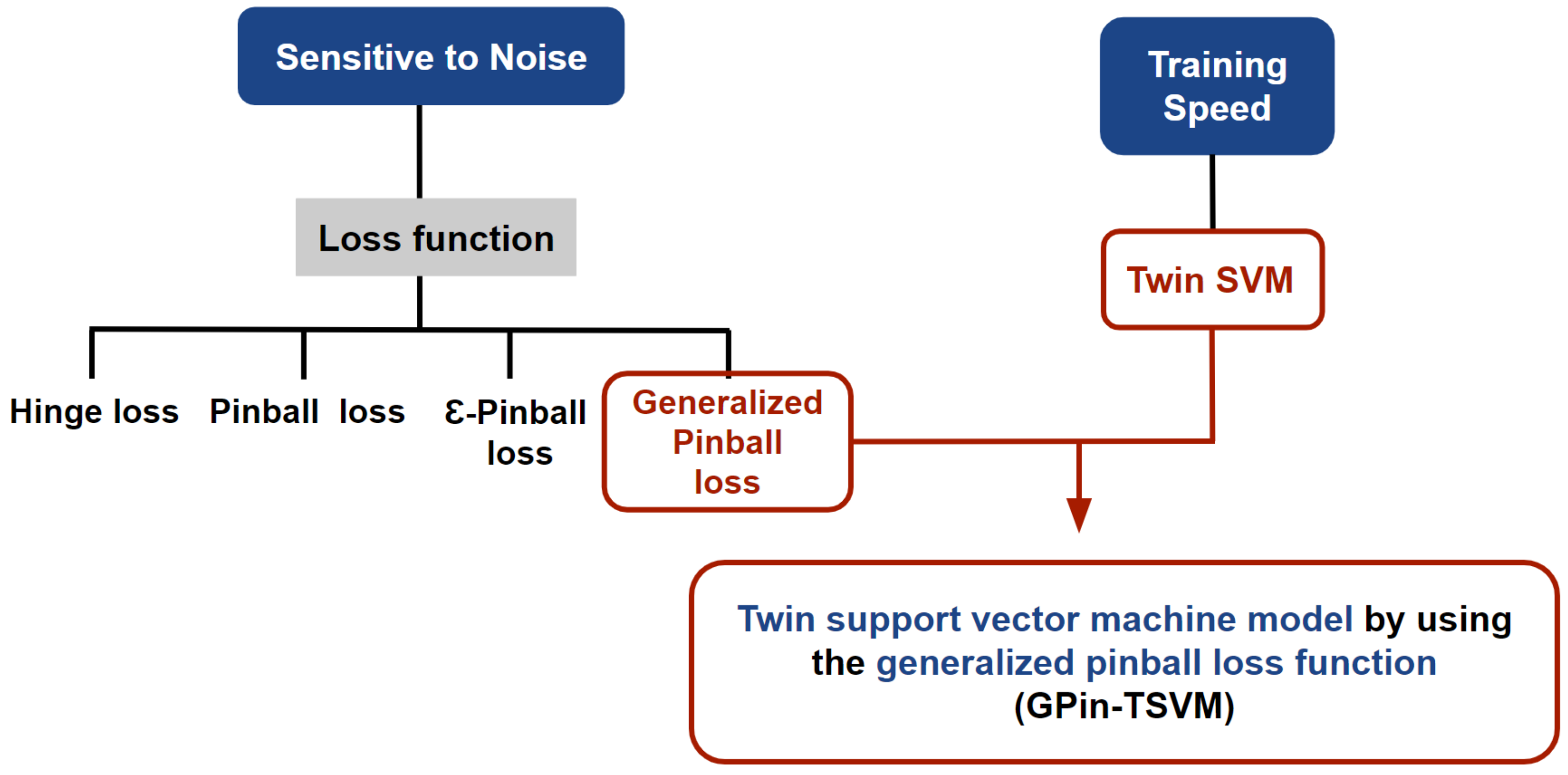
• For pattern classification, we add a generalized pinball loss function to the standard TSVM, resulting in a better classifier model that is called a generalized pinball loss function-based TSVM (GPin-TSVM);
• We demonstrate that the proposed algorithm GPin-TSVM surpasses existing classifiers in terms of accuracy in numerical experiments. We also examine its characteristics, such as noise sensitivity and within-class scatter;
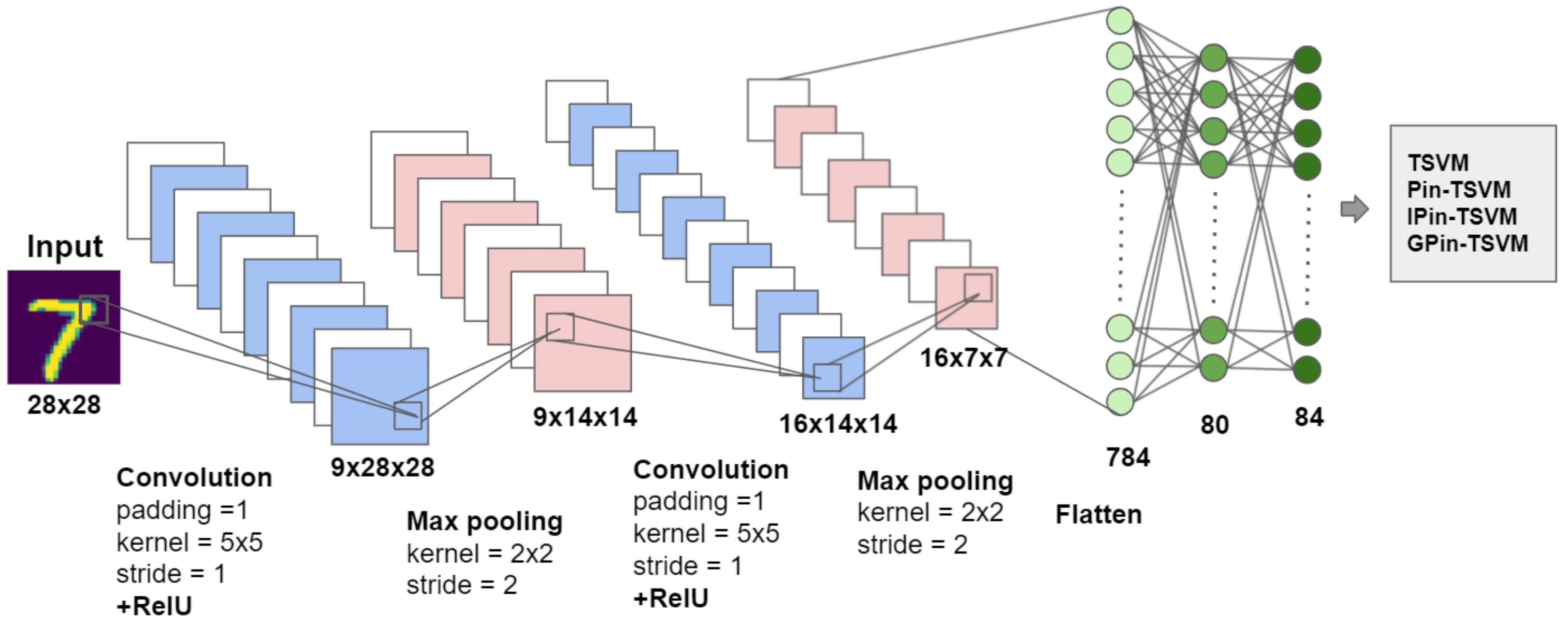
• We examine the applicability of the main techniques of GPin-TSVM toward handwritten digit recognition problems compared with the standard TSVM, Pin-TSVM, and $ϵ$-insensitive zone TSVM (IPin-TSVM). Moreover, we use the automatic feature extractor by the convolutional neural network (CNN) and TSVM, Pin-TSVM, IPin-SVM, and GPin-TSVM, which work as a binary classifier by replacing the softmax layer of CNN;
• We perform numerical testing on a synthetic dataset and datasets from numerous UCI benchmarks with noise of various variances to illustrate the validity of our proposed GPin-TSVM. The results also show the robustness of the proposed approach, which is less sensitive to noise and retains the sparsity of the solution.

In Section 2, we briefly discuss loss functions, SVM, generalized pinball SVM, and TSVM. In Section 3, we present a new approach called GPin-TSVM. In Section 4, the properties of the proposed GPin-TSVM are discussed. The efficiency of our proposed GPin-TSVM by using synthetic datasets and the UCI machine learning repository is compared to standard TSVM, Pin-TSVM, and IPin-TSVM, and the applications of the proposed GPin-TSVM algorithms in handwritten digit recognition are shown in Section 5. Conclusions and future recommendations are presented in Section 6.

2. Related Work and Background

In this section, standard SVM, TSVM, loss functions, and generalized pinball SVM formulations are briefly described. The interested readers are referred to [28,39,40,42] for a more detailed description.

2.1. Support Vector Machine

The difficulty of the SVM model lies in determining the optimal separating hyperplane, or maximal margin hyperplane, that best separates the two classes in order to generalize new data to obtain accurate classification predictions. Consider a two-class dataset of m data samples, where $S=\{(x_1,y_1),(x_2,y_2),\dots ,(x_m,y_m)\}$ for $i=1,2,\cdots ,m,x_i\in {\mathbb{R}}^n$ is the sample with the label $y_i\in \{1,-1\}$. SVM models receive a separating produced decision function $w^{\top }x+b=0$, where $w\in {\mathbb{R}}^n$ and $b\in \mathbb{R}$ from the following problem:

$$\begin{array}{ccc}\hfill \underset{w,b}{min}& & \frac{1}{2}{\parallel w\parallel }^2+C\sum _{i=1}^m{\xi }_i\hfill \\ \hfill \mathrm{s}.\mathrm{t}.& & 1-y_i(w^{\top }{x}_i+b)\ge 1-{\xi }_i,\hfill \\ & & {\xi }_i\ge 0,i=1,\dots ,m,\hfill \end{array}$$

(1)

where ${\xi }_i$ are the slack variables and C is the trade-off parameter. We obtain its dual QPP as follows by using the Lagrangian multipliers ${\alpha }_i$:

$$\begin{array}{ccc}\hfill & & \underset{\alpha }{min}\frac{1}{2}\sum _{i=1}^m\sum _{j=1}^m{y}_i{y}_j\left(x_i^{\top }{x}_j\right){\alpha }_i{\alpha }_j-\sum _{i=1}^m{\alpha }_i\hfill \\ & & \mathrm{s}.\mathrm{t}.\sum _{i=1}^m{y}_i{\alpha }_i=0,\hfill \\ & & 0\le {\alpha }_i\le C,i=1,\dots ,m.\hfill \end{array}$$

(2)

We use the number of support vectors that satisfy $0<\alpha <C$, represented by $N_{SV}$, and we obtain the following decision function after optimizing this dual QPP:

$$\begin{array}{c}\hfill y=\mathrm{sign}\left(\sum _{i=1}^{N_{SV}}{\alpha }_i^{*}{y}_i\left(x_i^{\top }x\right)+b\right)\end{array}$$

(3)

where ${\alpha }^{*}$ denotes the dual problem solution (2).

2.2. Twin Support Vector Machine

Consider the data set S, in which the matrix $A\in {\mathbb{R}}^{m_1\times n}$ represents $m_1$ data samples from class $+1$, and the matrix $B\in {\mathbb{R}}^{m_2\times n}$ represents $m_2$ data samples from class $-1$. The TSVM [28] is used to determine two nonparallel hyperplanes using the following definitions:

$$\begin{array}{c}\hfill x^{\top }{w}^{\left(1\right)}+b^{\left(1\right)}=0\mathrm{and}{x}^{\top }{w}^{\left(2\right)}+b^{\left(2\right)}=0\end{array}$$

(4)

where $w^{\left(1\right)},w^{\left(2\right)}\in {\mathbb{R}}^n$ and $b^{\left(1\right)},b^{\left(2\right)}\in \mathbb{R}$. To obtain the pair of nonparallel hyperplanes, the hinge loss function-based TSVM yields the following pair of QPPs:

$$\begin{array}{ccc}& & \underset{w^{\left(1\right)},b^{\left(1\right)},\xi }{min}\frac{1}{2}{\parallel A{w}^{\left(1\right)}+e_1{b}^{\left(1\right)}\parallel }^2+c_1{e}_2^{\top }\xi \hfill \\ & & \mathrm{s}.\mathrm{t}.-(B{w}^{\left(1\right)}+e_2{b}^{\left(1\right)})+\xi \ge e_2,\xi \ge 0,\hfill \\ \hfill \mathrm{and}\end{array}$$

(5)

$$\begin{array}{ccc}& & \underset{w^{\left(2\right)},b^{\left(2\right)},\xi }{min}\frac{1}{2}{\parallel B{w}^{\left(2\right)}+e_2{b}^{\left(2\right)}\parallel }^2+c_2{e}_1^{\top }\xi \hfill \\ & & \mathrm{s}.\mathrm{t}.(A{w}^{\left(2\right)}+e_1{b}^{\left(2\right)})+\xi \ge e_1,\xi \ge 0,\hfill \end{array}$$

(6)

where $c_1$ and $c_2$ are positive penalty parameters, $\xi$ is a slack variable, and $e_1$ and $e_2$ are vectors of appropriately sized ones. The dual of QPPs (5) and (6) can be represented, respectively, as follows:

$$\begin{array}{ccc}& & \underset{\alpha }{min}\frac{1}{2}{\alpha }^{\top }Q\left(P^{\top }P\right)Q^{\top }\alpha -e_2^{\top }\alpha \hfill \\ & & \mathrm{s}.\mathrm{t}.0\le \alpha \le c_1{e}_2\hfill \end{array}$$

(7)

and

$$\begin{array}{ccc}& & \underset{\beta }{min}\frac{1}{2}{\beta }^{\top }P\left(Q^{\top }Q\right)P^{\top }\beta -e_1^{\top }\beta \hfill \\ & & \mathrm{s}.\mathrm{t}.0\le \beta \le c_2{e}_1\hfill \end{array}$$

(8)

where $P=\left[\begin{array}{ccc}A& & e_1\end{array}\right]$ and $Q=\left[\begin{array}{ccc}B& & e_2\end{array}\right]$. From the solutions $\alpha$ and $\beta$ of (7) and (8), respectively, the best separating hyperplanes are given by:

$$\begin{array}{ccc}& & \left[\begin{array}{c}{w}^{\left(1\right)}\\ b^{\left(1\right)}\end{array}\right]=-{\left(P^{\top }P\right)}^{-1}{Q}^{\top }\alpha ,\hfill \end{array}$$

and

$$\begin{array}{ccc}& & \left[\begin{array}{c}{w}^{\left(2\right)}\\ b^{\left(2\right)}\end{array}\right]={\left(Q^{\top }Q\right)}^{-1}{P}^{\top }\beta .\hfill \end{array}$$

Depending on which of the two hyperplanes (4) a new sample point $x\in {\mathbb{R}}^n$ lies closest to, it is is assigned to class $i(i=+1\mathrm{or}-1)$ by

$$\begin{array}{c}\hfill \mathrm{class}\left(i\right)=\arg \underset{i=1,2}{min}\frac{|x^{\top }{w}^{\left(i\right)}+b^{\left(i\right)}|}{\parallel w^{\left(i\right)}\parallel }\end{array}$$

(9)

where $|.|$ denotes obtaining the absolute value. In actuality, the unconstrained optimization problem may be reformulated as the QPP of the TSVM problem (5) as follows [43]:

$$\begin{array}{c}\hfill \underset{w^{\left(1\right)},b^{\left(1\right)},\xi }{min}\frac{1}{2}{\parallel A{w}^{\left(1\right)}+e_1{b}^{\left(1\right)}\parallel }^2+c_1\sum _{i=1}^{m_2}{\mathcal{L}}_{hinge}\left(1+(x_i^{\top }{w}^{\left(1\right)}+b^{\left(1\right)})\right)\end{array}$$

(10)

and

$$\begin{array}{c}\hfill \underset{w^{\left(2\right)},b^{\left(2\right)},\xi }{min}\frac{1}{2}{\parallel B{w}^{\left(2\right)}+e_2{b}^{\left(2\right)}\parallel }^2+c_2\sum _{i=1}^{m_1}{\mathcal{L}}_{hinge}\left(1-(x_i^{\top }{w}^{\left(2\right)}+b^{\left(2\right)})\right),\end{array}$$

(11)

where ${\mathcal{L}}_{hinge}\left(u\right)=max\left\{0,u\right\}$ is known as the hinge loss function and $u=(1-y_i(x_i^{\top }w+b))$. The hinge loss is a loss function that is commonly used to train classifiers. Furthermore, it strives to optimize the shortest distance between two classes, resulting in resampling instability and noise sensitivity from the related classifier [42]. To deal with the problem of noise sensitivity, Huang [39] presented utilizing the pinball loss function by combining the SVM classifier with the pinball loss function. The pinball loss function explains how this approach works by penalizing correctly identified data as follows:

$$\begin{array}{c}\hfill {\mathcal{L}}_{pin}\left(u\right)=\left\{\begin{array}{cc}u,\hfill & u\ge 0,\hfill \\ -\tau u,\hfill & u<0,\hfill \end{array}\right.\end{array}$$

(12)

where $\tau \ge 0$ is a user-defined parameter. The so-called pinball loss is a well-known method in statistics and machine learning for calculating conditional quantiles. Despite achieving noise insensitivity, the pinball loss function is unable to achieve sparsity in the process. In their work, Huang examined a similar type of pinball loss function to ensure sparsity, which is a $ϵ$-insensitive pinball loss. The use of the $ϵ$-insensitive pinball loss function increases the prediction performance of the SVM model significantly. It also maintains sparsity in the SVM model. This function is defined as follows:

$$\begin{array}{c}\hfill {\mathcal{L}}_{pin}^{ϵ}\left(u\right)=\left\{\begin{array}{cc}u-ϵ,\hfill & u>ϵ,\hfill \\ 0,\hfill & -\frac{ϵ}{\tau }\le u\le ϵ,\hfill \\ -\tau \left(u+\frac{ϵ}{\tau }\right),\hfill & u<-\frac{ϵ}{\tau },\hfill \end{array}\right.\end{array}$$

(13)

where $\tau \ge 0$ and $ϵ\ge 0$ are user-defined parameters. In an SVM model, sparsity is well known to be a highly desirable property. A sparse SVM model constructs the decision function from a small number of training data points and predicts the responses of test data points in a very short amount of time. The width of the $ϵ$-insensitive zone function fluctuates with the $\tau$ values, but it should ideally change with the variation in the training data response values. In practicality, it also makes choosing a good $ϵ$-value difficult. As a result, Rastogi [40] saw the necessity to create an $ϵ$-insensitive pinball loss function that can be used to enhance the $ϵ$-insensitive method in SVM. They proposed an $({ϵ}_1,{ϵ}_2)$-insensitive zone pinball loss function by used this loss in combination with the SVM model. It is also called a generalized pinball SVM, with the following loss function:

$$\begin{array}{c}\hfill {\mathcal{L}}_{{\tau }_1,{\tau }_2}^{{ϵ}_1,{ϵ}_2}\left(u\right)=\left\{\begin{array}{cc}{\tau }_1\left(u-\frac{{ϵ}_1}{{\tau }_1}\right),\hfill & u>\frac{{ϵ}_1}{{\tau }_1},\hfill \\ 0,\hfill & -\frac{{ϵ}_2}{{\tau }_2}\le u\le \frac{{ϵ}_1}{{\tau }_1},\hfill \\ -{\tau }_2\left(u+\frac{{ϵ}_2}{{\tau }_2}\right),\hfill & u<-\frac{{ϵ}_2}{{\tau }_2},\hfill \end{array}\right.\end{array}$$

(14)

where ${\tau }_1,{\tau }_2,{ϵ}_1$, and ${ϵ}_2$ are non-negative parameters. In the next subsection, we briefly describe the generalized pinball SVM model that is proposed by Rastogi. This approach is a modification of previous loss functions that takes noise sensitivity, resampling stability, and data scatter minimization into account.

2.3. Support Vector Machine with Generalized Pinball Loss

With this generalized pinball loss function, the resulting formulation, termed as a generalized pinball support vector machine, is proposed by Rastogi [40], which results in the unconstrained optimization problem:

$$\begin{array}{c}\hfill \underset{w,b}{min}\frac{1}{2}{\parallel w\parallel }^2+\frac{C}{m}\sum _{i=1}^m{\mathcal{L}}_{{\tau }_1,{\tau }_2}^{{ϵ}_1,{ϵ}_2}\left(1-y_i(w^{\top }{x}_i+b)\right).\end{array}$$

(15)

Then, the problem (15) can reformulate to the following QPP:

$$\begin{array}{ccc}\hfill & & \underset{w,b,\xi }{min}\frac{1}{2}{\parallel w\parallel }^2+C\sum _{i=1}^m{\xi }_i\hfill \\ & & \mathrm{s}.\mathrm{t}.y_i(w^T{x}_i+b)\ge 1-\frac{1}{{\tau }_1}({\xi }_i+{ϵ}_1),\hfill \\ & & y_i(w^T{x}_i+b)\le 1+\frac{1}{{\tau }_2}({\xi }_i+{ϵ}_2),\hfill \\ & & {\xi }_i\ge 0,i=1,2,3,\dots ,m.\hfill \end{array}$$

(16)

Its dual QPP is generated as follows by inserting the Lagrangian multipliers ${\alpha }_i$ and ${\beta }_i$:

$$\begin{array}{ccc}\hfill \underset{\alpha ,\beta }{min}& & \frac{1}{2}\sum _{i=1}^m\sum _{j=1}^m({\alpha }_i-{\beta }_i)({\alpha }_j-{\beta }_j)y_i{y}_j\left(x_i^{\top }{x}_j\right)-(1-\frac{{ϵ}_1}{{\tau }_1})\sum _{i=1}^m{\alpha }_i+(1+\frac{{ϵ}_2}{{\tau }_2})\sum _{i=1}^m{\beta }_i\hfill \\ \hfill \mathrm{s}.\mathrm{t}.& & \sum _{i=1}^m({\alpha }_i-{\beta }_i)y_i=0,\hfill \\ & & 0\le \frac{{\alpha }_i}{{\tau }_1}+\frac{{\beta }_i}{{\tau }_2}\le C,i=1,\dots ,m.\hfill \end{array}$$

(17)

We can obtain the decision function (18) by solving the dual problem of (17):

$$\begin{array}{c}\hfill y=\mathrm{sign}\left(\sum _{i=1}^m({\alpha }_i^{*}-{\beta }_i^{*})y_i\left(x_i^{\top }x\right)+b\right).\end{array}$$

(18)

However, for large-scale applications, the generalized pinball SVM has a high computing complexity and is quite slow. In the next section, we go after the heart of our proposed technique, which is to reduce the high computational complexity by proposing a TSVM with a generalized pinball loss function that is aimed toward the binary classification problem, and to present both the linear and nonlinear cases, as shown in Figure 1.

3. Proposed Twin Support Vector Machine with Generalized Pinball Loss (GPin-TSVM)

In this section, we employ the Lagrange multiplier approach to derive the solution for our GPin-TSVM model, which is based on just the generalized pinball loss function. In both linear and nonlinear scenarios, our GPin-TSVM can be employed.

3.1. Linear Case

In the standard TSVM, we determine the generalized pinball loss and obtain the following QPPs:

$$\begin{array}{c}\hfill \underset{w^{\left(1\right)},b^{\left(1\right)}}{min}\frac{1}{2}{\parallel A{w}^{\left(1\right)}+e_1{b}^{\left(1\right)}\parallel }^2+c_1{e}_2^{\top }{\mathcal{L}}_{{\tau }_1,{\tau }_2}^{{ϵ}_1,{ϵ}_2}\left(e_2+(B{w}^{\left(1\right)}+e_2{b}^{\left(1\right)})\right)\end{array}$$

(19)

and

$$\begin{array}{c}\hfill \underset{w^{\left(2\right)},b^{\left(2\right)}}{min}\frac{1}{2}{\parallel B{w}^{\left(2\right)}+e_2{b}^{\left(2\right)}\parallel }^2+c_2{e}_1^{\top }{\mathcal{L}}_{{\tau }_3,{\tau }_4}^{{ϵ}_3,{ϵ}_4}\left(e_1-(A{w}^{\left(2\right)}+e_1{b}^{\left(2\right)})\right).\end{array}$$

(20)

The problems (19) and (20) are translated further into equivalent known formulations (5) and (6) by adding a slack vector $\xi$, yielding the following QPPs:

$$\begin{array}{ccc}& & \underset{w^{\left(1\right)},b^{\left(1\right)},\xi }{min}\frac{1}{2}{\parallel A{w}^{\left(1\right)}+e_1{b}^{\left(1\right)}\parallel }^2+c_1{e}_2^{\top }\xi \hfill \\ & & \mathrm{s}.\mathrm{t}.-(B{w}^{\left(1\right)}+e_2{b}^{\left(1\right)})\ge e_2-\frac{1}{{\tau }_1}(\xi +e_2{ϵ}_1),\hfill \\ & & -(B{w}^{\left(1\right)}+e_2{b}^{\left(1\right)})\le e_2+\frac{1}{{\tau }_2}(\xi +e_2{ϵ}_2),\hfill \\ & & \xi \ge 0,\hfill \end{array}$$

(21)

and

$$\begin{array}{ccc}& & \underset{w^{\left(2\right)},b^{\left(2\right)},\xi }{min}\frac{1}{2}{\parallel B{w}^{\left(2\right)}+e_2{b}^{\left(2\right)}\parallel }^2+c_2{e}_1^{\top }\xi \hfill \\ & & \mathrm{s}.\mathrm{t}.A{w}^{\left(2\right)}+e_1{b}^{\left(2\right)}\ge e_1-\frac{1}{{\tau }_3}(\xi +e_1{ϵ}_3),\hfill \\ & & A{w}^{\left(2\right)}+e_1{b}^{\left(2\right)}\le e_1+\frac{1}{{\tau }_4}(\xi +e_1{ϵ}_4),\hfill \\ & & \xi \ge 0,\hfill \end{array}$$

(22)

where ${\tau }_1,{\tau }_2,{\tau }_3,{\tau }_4,{ϵ}_1,{ϵ}_2,{ϵ}_3$, and ${ϵ}_4$ are non-negative parameters. We transform (21) and (22) to their dual form to arrive at the solution. For this, we use (21) and introduce the Lagrange multipliers $\alpha \ge 0,\beta \ge 0$, and $\gamma \ge 0$, and we obtain the Lagrange function:

$$\begin{array}{c}\hfill \mathcal{L}(w^{\left(1\right)},b^{\left(1\right)},\xi ,\alpha ,\beta ,\gamma )=\frac{1}{2}{\parallel A{w}^{\left(1\right)}+e_1{b}^{\left(1\right)}\parallel }^2+c_1{e}_2^{\top }\xi \\ \hfill -{\alpha }^{\top }\left(-(B{w}^{\left(1\right)}+e_2{b}^{\left(1\right)})-e_2+\frac{1}{{\tau }_1}(\xi +e_1{ϵ}_1)\right)-{\beta }^{\top }\xi \\ \hfill -{\gamma }^{\top }\left((B{w}^{\left(1\right)}+e_2{b}^{\left(1\right)})+e_2+\frac{1}{{\tau }_2}(\xi +e_2{ϵ}_2)\right).\end{array}$$

(23)

We use the KKT optimality conditions to find the following results:

$$\begin{array}{ccc}\hfill \frac{\partial \mathcal{L}}{\partial w^{\left(1\right)}}=A^{\top }(A{w}^{\left(1\right)}+e_1{b}^{\left(1\right)})+B^{\top }\alpha -B^{\top }\gamma & & =0,\hfill \end{array}$$

(24)

$$\begin{array}{ccc}\hfill \frac{\partial \mathcal{L}}{\partial b^{\left(1\right)}}=e_1^{\top }(A{w}^{\left(1\right)}+e_1{b}^{\left(1\right)})+e_2^{\top }\alpha -e_2^{\top }\gamma & & =0,\hfill \end{array}$$

(25)

$$\begin{array}{ccc}\hfill \frac{\partial \mathcal{L}}{\partial \xi }=c_1{e}_2-\frac{\alpha }{{\tau }_1}-\beta -\frac{\gamma }{{\tau }_2}& & =0,\hfill \end{array}$$

(26)

$$\begin{array}{ccc}\hfill {\alpha }^{\top }\left(-(B{w}^{\left(1\right)}+e_2{b}^{\left(1\right)})-e_2+\frac{1}{{\tau }_1}(\xi +e_1{ϵ}_1)\right)& & =0,\hfill \end{array}$$

(27)

$$\begin{array}{ccc}\hfill {\beta }^{\top }\xi & & =0,\hfill \end{array}$$

(28)

$$\begin{array}{ccc}\hfill {\gamma }^{\top }\left((B{w}^{\left(1\right)}+e_2{b}^{\left(1\right)})+e_2+\frac{1}{{\tau }_2}(\xi +e_2{ϵ}_2)\right)& & =0.\hfill \end{array}$$

(29)

By using (26) and $\beta \ge 0$, we obtain

$$\begin{array}{c}\hfill \frac{\alpha }{{\tau }_1}+\frac{\gamma }{{\tau }_2}\le c_1{e}_2\end{array}$$

(30)

Combining (24) and (25) yields

$$\begin{array}{c}\hfill \left[\begin{array}{c}{A}^{\top }\\ e_1^{\top }\end{array}\right]\left[\begin{array}{ccc}A& & e_1\end{array}\right]\left[\begin{array}{c}{w}^{\left(1\right)}\\ b^{\left(1\right)}\end{array}\right]-\left[\begin{array}{c}{B}^{\top }\\ e_2^{\top }\end{array}\right](\alpha -\gamma )=0.\end{array}$$

(31)

Define $\lambda =\alpha -\gamma ,P=\left[\begin{array}{ccc}A& & e_1\end{array}\right],$ and $Q=\left[\begin{array}{ccc}B& & e_2\end{array}\right]$. Equation (31) can be recast using these notations as follows:

$$\begin{array}{c}\hfill P^{\top }P\left[\begin{array}{c}{w}^{\left(1\right)}\\ b^{\left(1\right)}\end{array}\right]+Q^{\top }\lambda =0,\mathrm{i}.\mathrm{e}.,\left[\begin{array}{c}{w}^{\left(1\right)}\\ b^{\left(1\right)}\end{array}\right]=-{\left(P^{\top }P\right)}^{-1}{Q}^{\top }\lambda .\end{array}$$

(32)

We can obtain the dual of (21) using Equation (23) and the given KKT conditions as follows:

$$\begin{array}{ccc}\hfill \underset{\alpha ,\lambda }{min}& & \frac{1}{2}{\lambda }^{\top }Q{\left(P^{\top }P\right)}^{-1}{Q}^{\top }\lambda -{\lambda }^{\top }{e}_2(1+\frac{{ϵ}_2}{{\tau }_2})+{\alpha }^{\top }{e}_2\left(\frac{{ϵ}_1}{{\tau }_1}+\frac{{ϵ}_2}{{\tau }_2}\right)\hfill \\ \hfill \mathrm{s}.\mathrm{t}.& & 0\le \left(\frac{1}{{\tau }_1}+\frac{1}{{\tau }_2}\right)\alpha -\frac{\lambda }{{\tau }_2}\le c_1{e}_2,\hfill \\ & & \alpha \ge 0,\alpha -\lambda \ge 0.\hfill \end{array}$$

(33)

The dual problem of (22) can be derived similarly:

$$\begin{array}{ccc}\hfill \underset{\omega ,\mu }{min}& & \frac{1}{2}{\mu }^{\top }P{\left(Q^{\top }Q\right)}^{-1}{P}^{\top }\mu -{\mu }^{\top }{e}_1(1+\frac{{ϵ}_4}{{\tau }_4})+{\omega }^{\top }{e}_1\left(\frac{{ϵ}_3}{{\tau }_3}+\frac{{ϵ}_4}{{\tau }_4}\right)\hfill \\ \hfill \mathrm{s}.\mathrm{t}.& & 0\le \left(\frac{1}{{\tau }_3}+\frac{1}{{\tau }_4}\right)\omega -\frac{\mu }{{\tau }_4}\le c_2{e}_1,\hfill \\ & & \omega \ge 0,\mu \ge 0,\hfill \end{array}$$

(34)

where $\omega \ge 0$ and $\mu \ge 0$ are Lagrange multipliers. Finally, the best separating hyperplanes are given by:

$$\begin{array}{c}\hfill \left[\begin{array}{c}{w}^{\left(1\right)}\\ b^{\left(1\right)}\end{array}\right]=-{(P^{\top }P+\delta I)}^{-1}{Q}^{\top }\lambda ,\end{array}$$

and

$$\begin{array}{c}\hfill \left[\begin{array}{c}{w}^{\left(2\right)}\\ b^{\left(2\right)}\end{array}\right]={(Q^{\top }Q+\delta I)}^{-1}{P}^{\top }\mu .\end{array}$$

(35)

Since we cannot ensure $P^{\top }P$ and $Q^{\top }Q$ are irreversible, it is always positive semi-definite; however, in some circumstances, it may not be well conditioned. To account for the possibility of ill-conditioning of $P^{\top }P$ and $Q^{\top }Q$, the regularization term $\delta I(\delta >0)$ must be used [44]. Depending on which of the two hyperplanes (4) a new sample point $x\in {\mathbb{R}}^n$ lies closest to, it is assigned to class $i(i=+1\mathrm{or}$−1) by

$$\begin{array}{c}\hfill \mathrm{class}\left(i\right)=\arg \underset{i=1,2}{min}\frac{|x^{\top }{w}^{\left(i\right)}+b^{\left(i\right)}|}{\parallel w^{\left(i\right)}\parallel }.\end{array}$$

3.2. Nonlinear Case

In higher dimensions, support vector machines are even more difficult to interpret. It is considerably more difficult to view how the data can be separated linearly and what the decision boundary will look like. In practice, however, data are rarely linearly separable; therefore, we must transform it into a higher-dimensional space before developing a support vector classifier. This problem can be solved using the symmetric kernel trick. Now, we use a symmetric kernel method to extend our linear GPin-TSVM to the nonlinear case [28,45]. The symmetric kernels used have a significant impact on how well GPin-TSVM functions. The nonparallel hyperplanes in the kernel-generated space are as follows if the defined kernel function is $K(·,·)$:

$$\begin{array}{c}\hfill K(x^{\top },X^{\top })w^{\left(1\right)}+b^{\left(1\right)}=0\mathrm{and}K(x^{\top },X^{\top })w^{\left(2\right)}+b^{\left(2\right)}=0,\end{array}$$

(36)

where $w^{\left(1\right)},w^{\left(2\right)}\in {\mathbb{R}}^m$, and $X=\left[\begin{array}{c}{A}_{m_1\times n}\\ B_{m_1\times n}\end{array}\right]$. For the nonlinear case of the problems (21) and (22), the corresponding problems are

$$\begin{array}{ccc}& & \underset{w^{\left(1\right)},b^{\left(1\right)},\xi }{min}\frac{1}{2}\parallel K(A,X^{\top })w^{\left(1\right)}+e_1{b}^{\left(1\right)}\parallel +c_1{e}_2^{\top }\xi \hfill \\ & & \mathrm{s}.\mathrm{t}.-(K(B,X^{\top })w^{\left(1\right)}+e_2{b}^{\left(1\right)})\ge e_2-\frac{1}{{\tau }_1}(\xi +e_2{ϵ}_1),\hfill \\ & & -(K(B,X^{\top })w^{\left(1\right)}+e_2{b}^{\left(1\right)})\le e_2+\frac{1}{{\tau }_2}(\xi +e_2{ϵ}_2),\hfill \\ & & \xi \ge 0,\hfill \end{array}$$

(37)

and

$$\begin{array}{ccc}& & \underset{w^{\left(2\right)},b^{\left(2\right)},\xi }{min}\frac{1}{2}\parallel K(B,X^{\top })w^{\left(2\right)}+e_2{b}^{\left(2\right)}\parallel +c_2{e}_1^{\top }\xi \hfill \\ & & \mathrm{s}.\mathrm{t}.K(A,X^{\top })w^{\left(2\right)}+e_1{b}^{\left(2\right)}\ge e_1-\frac{1}{{\tau }_3}(\xi +e_1{ϵ}_3),\hfill \\ & & K(A,X^{\top })w^{\left(2\right)}+e_1{b}^{\left(2\right)}\le e_1+\frac{1}{{\tau }_4}(\xi +e_1{ϵ}_4),\hfill \\ & & \xi \ge 0.\hfill \end{array}$$

(38)

The Lagrange function is applied, and the KKT optimality requirements are used to produce the dual of (37):

$$\begin{array}{ccc}\hfill \underset{\alpha ,\gamma }{min}& & \frac{1}{2}{(\alpha -\gamma )}^{\top }Q{\left(P^{\top }P\right)}^{-1}{Q}^{\top }(\alpha -\gamma )-{(\alpha -\gamma )}^{\top }{e}_2(1+\frac{{ϵ}_2}{{\tau }_2})+{\alpha }^{\top }{e}_2\left(\frac{{ϵ}_1}{{\tau }_1}+\frac{{ϵ}_2}{{\tau }_2}\right)\hfill \\ \hfill \mathrm{s}.\mathrm{t}.& & \frac{\alpha }{{\tau }_1}+\frac{\gamma }{{\tau }_2}\le c_1{e}_1,\hfill \\ & & \alpha \ge 0,\alpha -\gamma \ge 0.\hfill \end{array}$$

(39)

Similarly, the dual of Equation (38) can be obtained as follows:

$$\begin{array}{ccc}\hfill \underset{\omega ,\mu }{min}& & \frac{1}{2}{(\omega -\mu )}^{\top }P{\left(Q^{\top }Q\right)}^{-1}{P}^{\top }(\omega -\mu )-{(\omega -\mu )}^{\top }{e}_1(1+\frac{{ϵ}_4}{{\tau }_4})+{\omega }^{\top }{e}_1\left(\frac{{ϵ}_3}{{\tau }_3}+\frac{{ϵ}_4}{{\tau }_4}\right)\hfill \\ \hfill \mathrm{s}.\mathrm{t}.& & \frac{\omega }{{\tau }_3}+\frac{\mu }{{\tau }_4}\le c_2{e}_1,\hfill \\ & & \omega \ge 0,\omega -\mu \ge 0,\hfill \end{array}$$

(40)

where $P=\left[\begin{array}{cc}K(A,X^{\top })& e_1\end{array}\right],Q=\left[\begin{array}{cc}K(B,X^{\top })& e_2\end{array}\right]$, and $\alpha ,\gamma ,\omega ,\mathrm{and}\mu$ are Lagrange multipliers. Finally, the best separating hyperplanes are given by:

$$\begin{array}{c}\hfill \left[\begin{array}{c}{w}^{\left(1\right)}\\ b^{\left(1\right)}\end{array}\right]=-{(P^{\top }P+\delta I)}^{-1}{Q}^{\top }(\alpha -\gamma )\end{array}$$

and

$$\begin{array}{c}\hfill \left[\begin{array}{c}{w}^{\left(2\right)}\\ b^{\left(2\right)}\end{array}\right]={(Q^{\top }Q+\delta I)}^{-1}{P}^{\top }(\omega -\mu ).\end{array}$$

(41)

Thus, a new sample point $x\in {\mathbb{R}}^n$ is assigned to class $i(i=+1\mathrm{or}-1)$ by

$$\begin{array}{c}\hfill \mathrm{class}\left(i\right)=\arg \underset{i=1,2}{min}\frac{|K(x^{\top },X^{\top })w^{\left(i\right)}+b^{\left(i\right)}|}{\parallel w^{\left(i\right)}\parallel }.\end{array}$$

4. Properties of the GPin-TSVM

We examine the noise insensitivity and within-class scatter properties of the GPin-TSVM in this section.

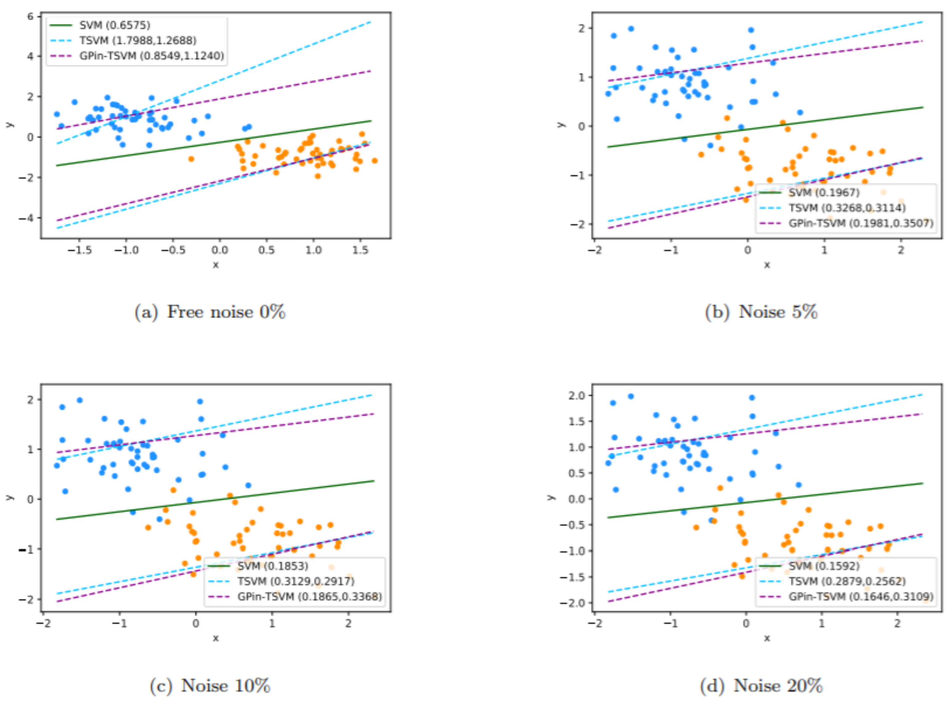
4.1. Noise Insensitivity

The principal advantage of our proposed algorithm GPin-TSVM is that it is insensitive to noise and maintains the sparsity. In this subsection, we explain the advantage of giving a penalty on a correctly classified point and conserving the sparsity to a certain scale at the same time. Consider the generalized sign function ${\mathrm{sgn}}_{{\tau }_1,{\tau }_2}^{{ϵ}_1,{ϵ}_2}(1-y(w^{\top }x+b))$ as

$${\mathrm{sgn}}_{{\tau }_1,{\tau }_2}^{{ϵ}_1,{ϵ}_2}\left(u\right)=\left\{\begin{array}{cc}\left\{{\tau }_1\right\},\hfill & u>\frac{{ϵ}_1}{{\tau }_1},\hfill \\ [0,{\tau }_1],\hfill & u=\frac{{ϵ}_1}{{\tau }_1},\hfill \\ \left\{0\right\},\hfill & -\frac{{ϵ}_2}{{\tau }_2}<u<\frac{{ϵ}_1}{{\tau }_1},\hfill \\ [-{\tau }_2,0],\hfill & u=-\frac{{ϵ}_2}{{\tau }_2},\hfill \\ \{-{\tau }_2\},\hfill & u<-\frac{{ϵ}_2}{{\tau }_2}.\hfill \end{array}\right.$$

(42)

${\mathrm{sgn}}_{{\tau }_1,{\tau }_2}^{{ϵ}_1,{ϵ}_2}\left(u\right)$ is the subgradient of (14). In the linear case, we will concentrate on the first model of the GPin-TSVM for clarity. Using the KKT optimality condition, Equation (19) can be written as:

$$\begin{array}{c}\hfill \mathbf{0}\in A^{\top }(A{w}^{\left(1\right)}+e_1{b}^{\left(1\right)})+c_1\sum _{i=1}^{m_2}{\mathrm{sgn}}_{{\tau }_1,{\tau }_2}^{{ϵ}_1,{ϵ}_2}(1+(w^{\left(1\right)}{x}_i^{-}+b^{\left(1\right)}))x_i^{-},\end{array}$$

(43)

where $\mathbf{0}$ is a zero vector. For the given $w^{\left(1\right)}$ and $b^{\left(1\right)}$, the entire index set can be divided into five different subsets:

$$\begin{array}{ccc}& & E_1^{+}=\left\{i:1+(w^{{\left(1\right)}^{\top }}{x}_i^{-}+b^{\left(1\right)})>\frac{{ϵ}_1}{{\tau }_1}\right\},\hfill \\ & & E_2^{+}=\left\{i:1+(w^{{\left(1\right)}^{\top }}{x}_i^{-}+b^{\left(1\right)})=\frac{{ϵ}_1}{{\tau }_1}\right\},\hfill \\ & & E_3^{+}=\left\{i:-\frac{{ϵ}_2}{{\tau }_2}<1+(w^{{\left(1\right)}^{\top }}{x}_i^{-}+b^{\left(1\right)})<\frac{{ϵ}_1}{{\tau }_1}\right\},\hfill \\ & & E_4^{+}=\left\{i:1+(w^{{\left(1\right)}^{\top }}{x}_i^{-}+b^{\left(1\right)})=-\frac{{ϵ}_2}{{\tau }_2}\right\},\hfill \\ & & E_5^{+}=\left\{i:1+(w^{{\left(1\right)}^{\top }}{x}_i^{-}+b^{\left(1\right)})<-\frac{{ϵ}_2}{{\tau }_2}\right\}.\hfill \end{array}$$

The data samples in $E_3^{+}$ may not benefit $w^{\left(1\right)}$ because the sub-gradient at all these datasets is zero, which is shown in Equation (42). As a result, $E_3^{+}$ has a direct impact on the model sparsity. We perceive that ${ϵ}_1$ and ${ϵ}_2$ control the number of samples in $E_3^{+}$. As ${ϵ}_1$ and ${ϵ}_2$ approach 0, sparsity is lost, whereas if ${ϵ}_1\to \infty$ and ${ϵ}_2\to \infty$, we increase the sparsity as a consequence of having more samples in $E_3^{+}$.

Using the notation $E_1^{+},E_2^{+},E_3^{+},E_4^{+}$, and $E_5^{+}$, Equation (43) can be rewritten as the existence of ${\psi }_i\in [0,{\tau }_1]$ and ${\theta }_i\in [-{\tau }_2,0]$, such that

$$\begin{array}{c}\hfill \frac{1}{c_1}{A}^{\top }(A{w}^{\left(1\right)}+e_1{b}^{\left(1\right)})+{\tau }_1\sum _{i\in E_1^{+}}{x}_i^{-}+\sum _{i\in E_2^{+}}{\psi }_i{x}_i^{-}+\sum _{i\in E_4^{+}}{\theta }_i{x}_i^{-}-{\tau }_2\sum _{i\in E_5^{+}}{x}_i^{-}=\mathbf{0}\end{array}$$

where $i=1,\dots ,m_2$.

Theorem 1.

Let $p_1$ be the number of samples $x_i^{-}$ in $E_1^{+}$. The following inequalities must hold if the optimization problems (33) or (39) have a solution:

$$\begin{array}{c}\hfill {\tau }_1+\frac{e_1^{\top }(A{w}^{\left(1\right)}+e_1{b}^{\left(1\right)})}{c_1{m}_2}\ge 0\end{array}$$

and

$$\begin{array}{c}\hfill \frac{p_1}{m_2}\le 1-\frac{{\tau }_1+\frac{e_1^{\top }(A{w}^{\left(1\right)}+e_1{b}^{\left(1\right)})}{c_1{m}_2}}{{\tau }_1+{\tau }_2}.\end{array}$$

Proof. 

Let $x_{i_0}^{-}$ be an arbitrary sample in $E_1^{+}$. We have ${\beta }_{i_0}={\gamma }_{i_0}=0$ by using the KKT condition (28) and (29). We obtain ${\alpha }_{i_0}=c_1{\tau }_1$ by using the KKT condition (26), which implies that ${\alpha }_{i_0}-{\gamma }_{i_0}=c_1{\tau }_1$. Let $\lambda =\alpha -\gamma$, which implies that ${\lambda }_{i_0}=c_1{\tau }_1$. In addition, we obtain $-e_1^{\top }(A{w}^{\left(1\right)}+e_1{b}^{\left(1\right)})=p_1{\gamma }_{i_0}+{\sum }_{i\notin E_1^{+}}{\lambda }_i=p_1{c}_1{\tau }_1+{\sum }_{i\notin E_1^{+}}{\lambda }_i$ from the KKT condition (25).

We can obtain $-c_1{\tau }_2\le {\lambda }_i\le c_1{\tau }_1$ because ${\alpha }_i\ge 0$ and ${\gamma }_i\ge 0$. As a result, we obtain

$$\begin{array}{c}\hfill -e_1^{\top }(A{w}^{\left(1\right)}+e_1{b}^{\left(1\right)})-{\tau }_1{c}_1(m_2-p_1)\le p_1{c}_1{\tau }_1\\ \hfill \le -e_1^{\top }(A{w}^{\left(1\right)}+e_1{b}^{\left(1\right)})+{\tau }_2{c}_1(m_2-p_1),\end{array}$$

thus, $-\frac{e_1^{\top }(A{w}^{\left(1\right)}+e_1{b}^{\left(1\right)})}{c_1{\tau }_1{m}_2}\le 1$ and $p_1\left(1+\frac{{\tau }_2}{{\tau }_1}\right)\le \frac{-e_1^{\top }(A{w}^{\left(1\right)}+e_1{b}^{\left(1\right)})+{\tau }_2{c}_1{m}_2}{c_1{\tau }_1}$. Finally, we have

$$\begin{array}{c}\hfill \frac{p_1}{m_2}\le \frac{1}{c_1({\tau }_1+{\tau }_2)}\left(\frac{-e_1^{\top }(A{w}^{\left(1\right)}+e_1{b}^{\left(1\right)})}{m_2}+{\tau }_2{c}_1\right)=1-\frac{{\tau }_1+\frac{e_1^{\top }(A{w}^{\left(1\right)}+e_1{b}^{\left(1\right)})}{c_1{m}_2}}{{\tau }_1+{\tau }_2}.\end{array}$$

□

Theorem 1 implies that $1-\frac{{\tau }_1+\frac{e_1^{\top }(A{w}^{\left(1\right)}+e_1{b}^{\left(1\right)})}{c_1{m}_2}}{{\tau }_1+{\tau }_2}$ is an upper boundary of the number of samples in $E_1^{+}$. The parameters ${\tau }_1$ and ${\tau }_2$ control the numbers of samples in $E_1^{+},E_3^{+}$, and $E_5^{+}$. When there is a decrease in ${\tau }_1$ and ${\tau }_2$, then the number of elements in $E_1^{+}$ becomes smaller and the classification result is sensitive to feature noise around the decision boundary, which will have a considerable impact. When ${\tau }_1$ and ${\tau }_2$ are both large, all three sets contain a large number of samples, making the outcome less sensitive to feature noise.

Briefly, parameters ${ϵ}_1,{ϵ}_2,{\tau }_1$, and ${\tau }_2$ control the tradeoff between sparsity and noise insensitivity. Similarly, we can separate the index set into the five sets on the second model of the GPin-TSVM:

$$\begin{array}{ccc}& & E_1^{-}=\left\{i:1-(w^{{\left(2\right)}^{\top }}{x}_i^{+}+b^{\left(2\right)})>\frac{{ϵ}_3}{{\tau }_3}\right\},\hfill \\ & & E_2^{-}=\left\{i:1-(w^{{\left(2\right)}^{\top }}{x}_i^{+}+b^{\left(2\right)})=\frac{{ϵ}_3}{{\tau }_3}\right\},\hfill \\ & & E_3^{-}=\left\{i:-\frac{{ϵ}_4}{{\tau }_4}<1-(w^{{\left(2\right)}^{\top }}{x}_i^{+}+b^{\left(2\right)})<\frac{{ϵ}_3}{{\tau }_3}\right\},\hfill \\ & & E_4^{-}=\left\{i:1-(w^{{\left(2\right)}^{\top }}{x}_i^{+}+b^{\left(2\right)})=-\frac{{ϵ}_4}{{\tau }_4}\right\},\hfill \\ & & E_5^{-}=\left\{i:1-(w^{{\left(2\right)}^{\top }}{x}_i^{+}+b^{\left(2\right)})<-\frac{{ϵ}_4}{{\tau }_4}\right\}\hfill \end{array}$$

where $i=1,\dots ,m_1$. Similar properties of the parameters ${\tau }_3$ and ${\tau }_4$ can be obtained as follows:

Theorem 2.

Let $p_2$ be the number of samples $x_i^{+}$ in $E_1^{-}$. If the optimization problems (34) or (40) have a solution, then the following inequalities must hold:

$$\begin{array}{c}\hfill {\tau }_3-\frac{e_2^{\top }(B{w}^{\left(2\right)}+e_2{b}^{\left(2\right)})}{c_2{m}_1}\ge 0\end{array}$$

and

$$\begin{array}{c}\hfill \frac{p_2}{m_1}\le 1-\frac{{\tau }_3-\frac{e_2^{\top }(B{w}^{\left(2\right)}+e_2{b}^{\left(2\right)})}{c_2{m}_1}}{{\tau }_3+{\tau }_4}.\end{array}$$

It also indicates that $1-\frac{{\tau }_3-\frac{e_2^{\top }(B{w}^{\left(2\right)}+e_2{b}^{\left(2\right)})}{c_2{m}_1}}{{\tau }_3+{\tau }_4}$ is an upper bound on the number of samples in $E_1^{-}$.

4.2. Scatter Minimization

Scatter minimization can also be used to understand the GPin-TSVM. For simplicity, consider only the first QPP (19) of the GPin-TSVM. The conclusions for another QPP (20) can also be obtained in this manner. For the given $x_i^{-}\in B$ and $x_j^{+}\in A$, the positive hyperplane $x^{\top }{w}^{\left(1\right)}+b^{\left(1\right)}=0$ can be established by data samples under the subset $Y_2^{+}\subseteq A$, and the two hyperplanes ${\mathcal{H}}^{+}=\{w^{{\left(1\right)}^{\top }}{x}_i^{-}+b^{\left(1\right)}+1=0\}$ and ${\mathcal{H}}^{-}=\{w^{{\left(2\right)}^{\top }}{x}_j^{+}+b^{\left(2\right)}-1=0\}$ are defined by data samples in subsets $Y_3^{+}\subseteq E_3^{+}$ and subset $Y_3^{-}\subseteq E_3^{-}$, respectively.

The scatter is calculated by adding the distances between each point $x_i^{-}$ and one supplied negative sample $x_{i_3}^{-}\in Y_3^{+}$. The scatter of $x_i^{-}\in B$ around the sample $x_{i_3}^{-}$ can be determined as

$$\begin{array}{c}\hfill \sum _{i=1}^{m_2}|w^{{\left(1\right)}^{\top }}{x}_{i_3}^{-}+b^{\left(1\right)}-(w^{{\left(1\right)}^{\top }}{x}_i^{-}+b^{\left(1\right)})|=\sum _{i=1}^{m_2}\left|w^{{\left(1\right)}^{\top }}(x_{i_3}^{-}-x_i^{-})\right|.\end{array}$$

(44)

We obtain the following equation by using $w^{{\left(1\right)}^{\top }}{x}_{i_3}^{-}+b^{\left(1\right)}+1=0$:

$$\begin{array}{ccc}\hfill \sum _{i=1}^{m_2}|w^{{\left(1\right)}^{\top }}(x_{i_3}^{-}-x_i^{-})|& & =\sum _{i=1}^{m_2}|w^{{\left(1\right)}^{\top }}{x}_{i_3}^{-}+b^{\left(1\right)}-(w^{{\left(1\right)}^{\top }}{x}_i^{-}+b^{\left(1\right)})|\hfill \\ & & =\sum _{i=1}^{m_2}|-1-(w^{{\left(1\right)}^{\top }}{x}_i^{-}+b^{\left(1\right)})|\hfill \\ & & =\sum _{i=1}^{m_2}|1+(w^{{\left(1\right)}^{\top }}{x}_i^{-}+b^{\left(1\right)})|.\hfill \end{array}$$

Similarly, using a specific data sample $x_{j_2}^{+}\in Y_2^{+}$, the scatter for every sample $x_j^{+}\in A$ is calculated as follows:

$$\begin{array}{ccc}\hfill \sum _{j=1}^{m_1}\left|w^{{\left(1\right)}^{\top }}(x_{j_2}^{+}-x_j^{+})\right|& & =\sum _{j=1}^{m_1}|w^{{\left(1\right)}^{\top }}{x}_{j_2}^{+}+b^{\left(1\right)}-(w^{{\left(1\right)}^{\top }}{x}_j^{+}+b^{\left(1\right)})|\hfill \\ & & =\sum _{i=1}^{m_1}|-(w^{{\left(1\right)}^{\top }}{x}_j^{+}+b^{\left(1\right)})|\hfill \end{array}$$

where $w^{{\left(1\right)}^{\top }}{x}_{j_2}^{+}+b^{\left(1\right)}=0$. Due to the fact that the scatter is a positive value, we can take it as the sum of squares, i.e., ${\sum }_{i=1}^{m_1}{(-(w^{{\left(1\right)}^{\top }}{x}_j^{+}+b^{\left(1\right)}))}^2$.

Consider the formula as follows:

$$\begin{array}{c}\hfill \underset{w^{\left(1\right)},b^{\left(1\right)}}{min}\frac{1}{2}\sum _{i=1}^{m_1}{(-(w^{{\left(1\right)}^{\top }}{x}_j^{+}+b^{\left(1\right)}))}^2+c_{11}\sum _{i=1}^{m_2}|1+(w^{{\left(1\right)}^{\top }}{x}_i^{-}+b^{\left(1\right)})|\end{array}$$

(45)

where $c_{11}$ is a constant. This guarantees that the first term may be expressed in such a way that the scatters $x_j^{+}\in A$ about the hyperplane $x^{\top }{w}^{\left(1\right)}+b^{\left(1\right)}=0$ are minimized. Nevertheless, this second term seeks to lower the error values caused according to how close B samples must be to ${\mathcal{H}}^{+}$ by minimizing the scatter of $x_i^{-}\in B$ from around hyperplane ${\mathcal{H}}^{+}$.

In the GPin-TSVM (19), the first term of (45) is mentioned in its mathematically equivalent form, whereas the absolute value used in (45) is extended to ${\mathcal{L}}_{{\tau }_1,{\tau }_2}^{{ϵ}_1,{ϵ}_2}$.

The first term of (45) is expressed within GPin-TSVM (19) in its mathematically equivalent form, whereas the absolute value employed in (45) is extended to ${\mathcal{L}}_{{\tau }_1,{\tau }_2}^{{ϵ}_1,{ϵ}_2}$. Concretely, we introduce the misclassification term

$$\begin{array}{ccc}& & c_{12}{\mathcal{L}}_{hinge}\left(1+(w^{{\left(1\right)}^{\top }}{x}_i^{-}+b^{\left(1\right)})-\frac{{ϵ}_1}{{\tau }_1}\right)=c_{12}max\left\{0,1+(w^{{\left(1\right)}^{\top }}{x}_i^{-}+b^{\left(1\right)})-\frac{{ϵ}_1}{{\tau }_1}\right\}\hfill \\ & & c_{13}{\mathcal{L}}_{hinge}(1+(w^{{\left(1\right)}^{\top }}{x}_i^{-}+b^{\left(1\right)}))=c_{13}max\{0,1+(w^{{\left(1\right)}^{\top }}{x}_i^{-}+b^{\left(1\right)})\}\hfill \\ & & c_{14}{\mathcal{L}}_{hinge}(-1-(w^{{\left(1\right)}^{\top }}{x}_i^{-}+b^{\left(1\right)}))=c_{14}max\{0,-1-(w^{{\left(1\right)}^{\top }}{x}_i^{-}+b^{\left(1\right)})\}\hfill \\ & & c_{15}{\mathcal{L}}_{hinge}\left(-1-(w^{{\left(1\right)}^{\top }}{x}_i^{-}+b^{\left(1\right)})-\frac{{ϵ}_2}{{\tau }_2}\right)=c_{15}max\left\{0,-1-(w^{{\left(1\right)}^{\top }}{x}_i^{-}+b^{\left(1\right)})-\frac{{ϵ}_2}{{\tau }_2}\right\}\hfill \end{array}$$

into (45), where $c_{12},c_{13},c_{14}$ and $c_{15}$ are positive parameters; that is,

$$\begin{array}{c}\hfill \underset{w^{\left(1\right)},b^{\left(1\right)}}{min}\frac{1}{2}\sum _{i=1}^{m_1}{(-(w^{{\left(1\right)}^{\top }}{x}_j^{+}+b^{\left(1\right)}))}^2+c_{11}\sum _{i=1}^{m_2}|1+(w^{{\left(1\right)}^{\top }}{x}_i^{-}+b^{\left(1\right)})|\\ \hfill +c_{12}\sum _{i=1}^{m_2}{\mathcal{L}}_{hinge}(1+(w^{{\left(1\right)}^{\top }}{x}_i^{-}+b^{\left(1\right)})-\frac{{ϵ}_1}{{\tau }_1})+c_{13}\sum _{i=1}^{m_2}{\mathcal{L}}_{hinge}(1+(w^{{\left(1\right)}^{\top }}{x}_i^{-}+b^{\left(1\right)}))\\ \hfill +c_{14}\sum _{i=1}^{m_2}{\mathcal{L}}_{hinge}(-1-(w^{{\left(1\right)}^{\top }}{x}_i^{-}+b^{\left(1\right)}))+c_{15}\sum _{i=1}^{m_2}{\mathcal{L}}_{hinge}\left(-1-(w^{{\left(1\right)}^{\top }}{x}_i^{-}+b^{\left(1\right)})-\frac{{ϵ}_2}{{\tau }_2}\right).\end{array}$$

The GPin-TSVM (19) can be obtained using the following conditions: $c_{11}+c_{12}+c_{13}=c_1{\tau }_1,c_{11}+c_{13}=0,c_{11}+c_{14}=0$, and $c_{11}+c_{14}+c_{15}=c_1{\tau }_2$. We have ${\tau }_1=\frac{c_{12}}{c_1}$ and ${\tau }_2=\frac{c_{15}}{c_1}$ from the first and last condition. The interpretation of this report is that the reasonable range of ${\tau }_1\ge 0$ and ${\tau }_2\ge 0$. We examine the misclassification error and the within-class scatter of one class simultaneously in the generalized pinball loss minimization. The GPin-TSVM (19) is then regarded as a trade-off between low misclassification and reduced scatter.

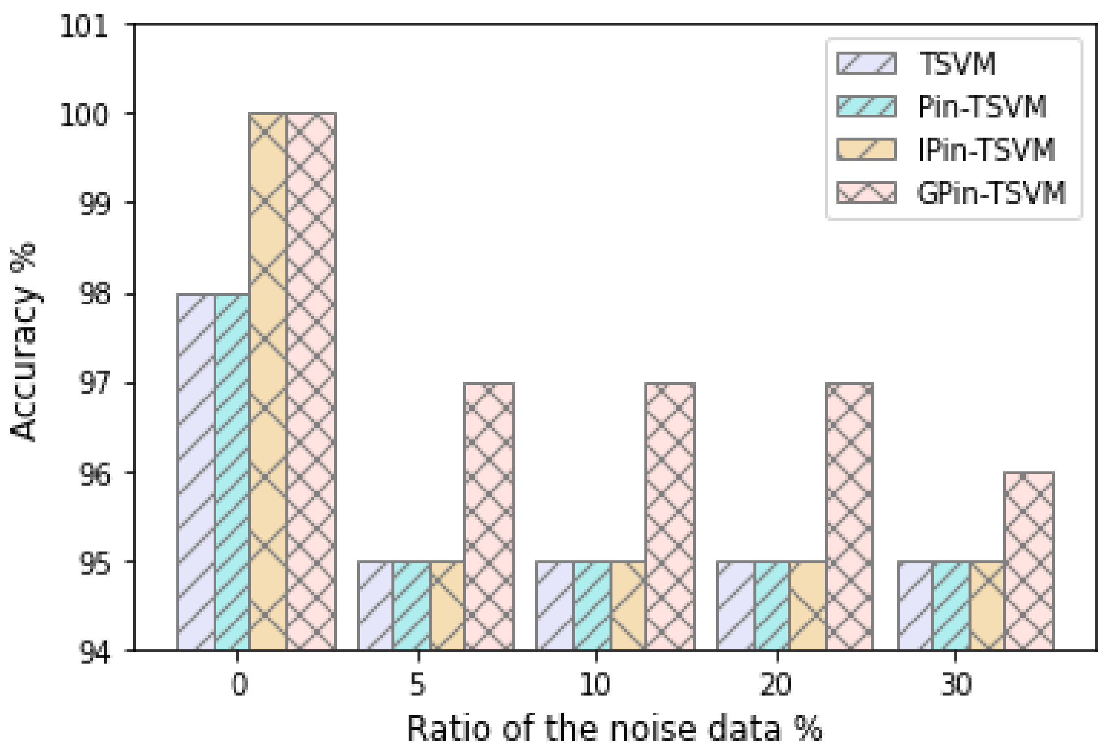
5. Numerical Experiments

In this section, the classification performance of the proposed approach in terms of accuracy is compared to that of other relevant approaches, such as the hinge loss twin support vector machine (TSVM), pinball loss TSVM (Pin-TSVM), and $ϵ$- insensitive loss TSVM (IPin-TSVM), on synthetic datasets and the UCI machine learning repository [46], and handwritten digit recognition applications have been proposed. We employed 10-fold cross validation for all of our experiments. The average accuracy and standard deviation for each experiment are displayed in all tables, with the best one highlighted.

All experiments are implemented in Python 3.9.5. on Windows 8 running on a 1.9 GHz laptop with 4 GB RAM with system configuration Intel Core i5+ Duo CPU E7500 (2.93 GHz). From now on, we denote ${\tau }_1={\tau }_3$, ${\tau }_2={\tau }_4$, ${ϵ}_1={ϵ}_3$, and ${ϵ}_2={ϵ}_4$. To derive the nonlinear case, we use the radial basis function kernel $K(x,y)=exp\{-\frac{{\parallel x-y\parallel }^2}{2\sigma }\}$.

5.1. Synthetic Dataset

We test our approach on a two-dimensional case in which equal samples are drawn from two Gaussian distributions: $x_i,i\in \{i:y_i=1\}\sim \mathcal{N}({\mu }_1,{\mathsf{\Sigma }}_1)$ and $x_i,i\in \{i:y_i=-1\}\sim \mathcal{N}({\mu }_2,{\mathsf{\Sigma }}_2)$, where ${\mu }_1={[1,-3]}^{\top },{\mu }_2={[-1,3]}^{\top }$ and ${\mathsf{\Sigma }}_1={\mathsf{\Sigma }}_2=\left[\begin{array}{cc}0.2& 0\\ 0& 3\end{array}\right]$. In order to make the dataset more interesting, we introduce noise. The labels of the noise points are chosen with equal probabilities from $\{1,-1\}$. The placements of these samples match the Gaussian distribution $\mathcal{N}({\mu }_n,{\mathsf{\Sigma }}_n)$, where ${\mu }_n={[0,0]}^{\top }$ and ${\mathsf{\Sigma }}_n=\left[\begin{array}{cc}1& -0.8\\ -0.8& 1\end{array}\right]$. The labels around the decision boundaries are affected by the noise. The ratio of noise data in the training set is represented by r. From Figure 2, the bar chart demonstrates the percentages of the accuracy of classifying different sectors, including GPin-TSVM, IPin-TSVM, Pin-TSVM, and TSVM during $r=0\%$ to $30\%$. In the large majority of cases, the GPin-TSVM produces the greatest outcome. This implies that the GPin-TSVM was the strongest candidate for the method of classifying the noise-corrupted data.

In the next result in Figure 3, we show the obtained value of the slopes of hyperplanes over four different noisy synthetic datasets by SVM, TSVM, and the proposed GPin-TSVM. In this result, we show that, when the level of noise increases from 0 to 20%, the hyperplanes of SVM diverge from 0.6575 to 0.1592 and the hyperplanes of TSVM diverge from 1.7988, 1.2688 to 0.2879, 0.2562, whereas the hyperplanes of our GPin-TSVM slightly changes. This suggests that our proposed GPin-TSVM model is unaffected by noise near the boundary.

5.2. UCI Datasets

Additionally, we perform testing on 10 benchmark datasets from the UCI machine learning database [46]. Imbalanced datasets lead to incorrect classification in classification problems. The imbalance ratio (IR) [47] is defined as the ratio of the number of data points on the majority class to the number of data points on the minority class.

$$\begin{array}{c}\hfill \mathrm{IR}=\frac{\mathrm{number}\mathrm{of}\mathrm{data}\mathrm{points}\mathrm{on}\mathrm{the}\mathrm{majority}\mathrm{class}}{\mathrm{number}\mathrm{of}\mathrm{data}\mathrm{points}\mathrm{on}\mathrm{the}\mathrm{minority}\mathrm{class}}.\end{array}$$

(46)

The dataset descriptions can be found in

Table 1. UCI datasets are described in detail.

Datasets	#Features	#Samples	IR
Breast	10	116	1.23
Planning relax	12	182	2.5
Ionosphere	33	351	1.79
Heart-Statlog	13	270	1.25
Heart-C	13	303	1.19
Spect	22	267	3.85
Saheart	9	462	1.89
WDBC	30	569	1.68
Pima-Indian	8	768	1.86
Australian	14	690	1.25

. To modify the tradeoff parameters and kernel parameter $\sigma$ for UCI benchmark datasets, we used the grid search method [48]. A validation set of 10% randomly selected data points was used for each dataset. We chose values for parameters $c_1$ and $c_2$ from the set $\left\{{10}^i\right|i=-2,-1,0,1,2\}$ for our tests. Further, another parameter was tuned in the range $\{0.1,0.25,0.5,0.75,1,1.5,2,2.5\}$.

Table 2. On UCI datasets, 10-fold cross validation using the linear kernel yielded the mean accuracy (%) and standard deviation.

Datasets	r	Existing Algorithm			Proposed Algorithm
		TSVM	Pin-TSVM	IPin-TSVM	GPin-TSVM
Breast	0	69.02 ± 8.61	69.85 ± 7.92	72.73 ± 16.79	71.67 ± 15.53
	0.05	69.02 ± 8.46	69.02 ± 8.61	72.73 ± 16.79	71.74 ± 15.45
	0.1	68.03 ± 8.09	68.26 ± 11.86	73.56 ± 14.44	73.41 ± 14.32
	0.2	69.85 ± 10.08	70.08 ± 13.15	71.82 ± 15.82	71.82 ± 14.56
Planning relax	0	71.61 ± 13.78	71.61 ± 13.78	71.61 ± 13.78	71.61 ± 13.78
	0.05	71.61 ± 13.78	71.61 ± 13.78	71.61 ± 13.78	71.61 ± 13.78
	0.1	71.61 ± 13.78	71.05 ± 13.41	71.61 ± 13.78	72.16 ± 13.68
	0.2	71.61 ± 13.78	72.69 ± 13.95	71.61 ± 13.78	71.61 ± 13.78
Australian	0	86.09 ± 3.56	86.38 ± 4.45	86.96 ± 3.72	86.81 ± 3.69
	0.05	85.36 ± 4.02	86.23 ± 4.50	85.80 ± 4.57	87.39 ± 3.43
	0.1	85.22 ± 3.71	85.51 ± 3.67	85.36 ± 5.16	88.26 ± 4.02
	0.2	83.91 ± 4.91	85.22 ± 4.04	84.93 ± 4.55	86.81 ± 3.69
Heart-Statlog	0	84.07 ± 8.12	83.33 ± 7.45	83.70 ± 9.40	83.33 ± 6.47
	0.05	83.33 ± 8.32	83.70 ± 8.15	83.33 ± 9.69	84.44 ± 6.99
	0.1	83.70 ± 8.15	82.59 ± 7.95	83.70 ± 9.54	84.07 ± 7.04
	0.2	84.44 ± 8.08	83.33 ± 7.08	81.11 ± 9.86	83.70 ± 8.80
Saheart	0	71.64 ± 5.01	71.01 ± 7.40	72.08 ± 5.34	72.93 ± 6.37
	0.05	71.63 ± 5.50	70.58 ± 7.51	71.86 ± 4.43	72.71 ± 6.59
	0.1	72.51 ± 5.84	70.37 ± 7.25	71.86 ± 5.90	72.06 ± 5.94
	0.2	71.21 ± 5.58	69.93 ± 6.00	71.00 ± 5.28	71.64 ± 5.39
WDBC	0	95.43 ± 1.61	95.96 ± 1.37	96.31 ± 2.54	97.19 ± 1.61
	0.05	94.20 ± 3.34	94.03 ± 3.16	95.08 ± 3.02	96.13 ± 2.04
	0.1	93.32 ± 2.19	92.97 ± 3.68	93.50 ± 3.05	95.60 ± 1.97
	0.2	93.32 ± 2.19	92.44 ± 1.93	93.32 ± 2.57	94.55 ± 1.46
Pima	0	76.83 ± 3.71	76.70 ± 3.36	76.57 ± 4.12	77.22 ± 4.07
	0.05	76.70 ± 3.74	76.31 ± 3.53	76.44 ± 3.66	76.96 ± 3.81
	0.1	76.44 ± 4.29	77.22 ± 3.30	77.09 ± 3.96	76.44 ± 3.87
	0.2	76.18 ± 3.62	76.83 ± 3.23	77.22 ± 4.03	76.18 ± 3.73
Ionosphere	0	90.60 ± 3.61	91.46 ± 3.10	90.90 ± 5.20	92.31 ± 2.87
	0.05	87.47 ± 6.28	90.31 ± 2.92	88.89 ± 4.51	90.88 ± 3.34
	0.1	87.44 ± 5.90	86.88 ± 5.90	86.62 ± 5.83	89.18 ± 5.05
	0.2	84.34 ± 5.85	85.47 ± 5.64	84.91 ± 4.38	87.16 ± 5.17

and

Table 3. On UCI datasets, 10-fold cross validation using the RBF kernel yielded the mean accuracy (%) and standard deviation.

Datasets	r	Existing Algorithm			Proposed Algorithm
		TSVM	Pin-TSVM	IPin-TSVM	GPin-TSVM
Breat	0	74.24 ± 11.23	74.24 ± 11.23	78.71 ± 12.47	74.24 ± 12.16
	0.05	74.24 ± 11.23	74.24 ± 11.23	80.38 ± 10.61	74.32 ± 13.35
	0.1	73.33 ± 12.36	74.32 ± 10.34	80.38 ± 11.25	73.41 ± 11.79
	0.2	73.41 ± 13.15	73.33 ± 12.36	77.80 ± 12.09	75.15 ± 13.63
Spect	0	83.50 ± 6.15	84.25 ± 6.31	84.23 ± 7.00	84.63 ± 7.05
	0.05	83.12 ± 5.69	83.49 ± 6.60	84.62 ± 6.46	84.63 ± 6.43
	0.1	82.75 ± 5.69	83.15 ± 7.32	83.87 ± 6.97	84.64 ± 7.72
	0.2	82.02 ± 5.22	82.01 ± 6.96	83.12 ± 7.05	83.29 ± 7.43
Australian	0	86.81 ± 2.93	86.67 ± 3.60	86.96 ± 3.94	86.67 ± 4.19
	0.05	82.46 ± 4.02	84.78 ± 3.90	86.81 ± 4.27	87.39 ± 3.11
	0.1	82.61 ± 2.59	82.90 ± 4.93	86.38 ± 3.32	86.52 ± 3.61
	0.2	82.32 ± 3.42	82.46 ± 4.74	85.51 ± 2.67	85.65 ± 3.63
Heart-Statlog	0	84.44 ± 7.73	84.81 ± 7.49	83.33 ± 8.32	84.81 ± 7.49
	0.05	84.07 ± 7.60	84.44 ± 8.08	84.81 ± 8.36	84.81 ± 7.49
	0.1	84.07 ± 7.95	84.44 ± 6.99	83.70 ± 8.31	84.44 ± 7.91
	0.2	84.07 ± 7.23	82.59 ± 7.60	84.07 ± 7.42	84.07 ± 6.84
Heart-C	0	82.85 ± 4.52	82.23 ± 8.94	82.85 ± 4.79	82.90 ± 8.36
	0.05	82.19 ± 5.04	81.25 ± 8.30	81.87 ± 4.08	82.54 ± 7.08
	0.1	81.56 ± 7.04	80.89 ± 6.77	81.89 ± 6.09	82.53 ± 4.59
	0.2	80.23 ± 5.95	80.81 ± 5.79	80.23 ± 4.55	82.18 ± 5.46
WDBC	0	97.54 ± 1.17	97.71 ± 1.58	97.89 ± 1.32	97.89 ± 1.32
	0.05	95.61 ± 2.51	95.79 ± 2.24	95.61 ± 1.96	95.60 ± 2.26
	0.1	95.08 ± 3.12	95.08 ± 2.91	95.78 ± 2.74	95.08 ± 2.58
	0.2	93.49 ± 2.75	93.85 ± 1.79	94.03 ± 2.24	94.20 ± 2.72
Ionosphere	0	96.02 ± 2.58	95.17 ± 3.60	95.16 ± 2.23	95.15 ± 4.05
	0.05	95.17 ± 3.12	94.60 ± 3.91	94.87 ± 2.49	94.59 ± 3.24
	0.1	94.60 ± 3.22	94.60 ± 2.67	94.87 ± 3.07	94.31 ± 3.36
	0.2	93.46 ± 3.09	92.60 ± 2.91	92.59 ± 4.09	93.48 ± 4.44
Pima	0	77.09 ± 3.31	76.96 ± 3.20	77.35 ± 3.71	77.48 ± 3.33
	0.05	76.96 ± 3.45	76.83 ± 3.34	76.70 ± 3.01	76.96 ± 3.83
	0.1	76.57 ± 2.51	75.66 ± 3.14	75.92 ± 3.42	76.43 ± 2.68
	0.2	75.53 ± 1.65	76.18 ± 3.51	76.05 ± 2.82	76.57 ± 3.16

summarize the experimental results of four approaches (TSVM, Pin-TSVM, IPin-SVM, and GPin-TSVM) on linear and RBF kernels, respectively. The optimal parameters used in Table 2 and Table 3 are summarized in

Table 4. The optimal parameters of Table 2.

Datasets	TSVM	Pin-TSVM	IPin-TSVM	GPin-TSVM
	${\mathit{c}}_{\mathit{1}},{\mathit{c}}_{\mathit{2}}$	${\mathit{c}}_{\mathit{1}},{\mathit{c}}_{\mathit{2}},\mathit{\tau }$	${\mathit{c}}_{\mathit{1}},{\mathit{c}}_{\mathit{2}},\mathit{\tau },\mathit{ϵ}$	${\mathit{c}}_{\mathit{1}},{\mathit{c}}_{\mathit{2}},{\mathit{\tau }}_{\mathit{1}},{\mathit{\tau }}_{\mathit{2}},$ ${\mathit{ϵ}}_{\mathit{1}},{\mathit{ϵ}}_{\mathit{2}}$
Breast	0.01, 0.01	0.01, 0.01, 1	10, 0.01, 1, 1	0.01, 0.01, 0.75, 0.5, 0.1, 0.1
Planning relax	0.1, 1	0.1, 1, 0.1	0.1, 1, 0.1, 0.1	0.1, 0.1, 1, 0.1, 0.1, 0.1
Australian	1, 0.1	0.1, 0.1, 0.5	1, 0.1, 0.1, 1	1, 0.1, 1, 0.5, 0.1, 0.1
Heart-Statlog	0.1, 0.1	1, 1, 1	1, 10, 0.5, 1	1, 10, 1, 0.5, 0.1, 0.5
Saheart	0.1, 0.1	1, 1, 1	1, 1, 1, 0.1	1, 1, 1.5, 0.5, 0.5, 0.1
WDBC	0.01, 0.01	0.1, 0.1, 0.1	1, 10, 0.1, 0.5	0.01, 0.01, 2, 1, 0.5, 0.1
Pima	0.1, 0.1	0.1, 0.1, 1.5	1, 1, 1, 0.1	1, 1, 1, 0.5, 0.1, 0.1
Ionosphere	0.01, 0.01	0.1, 0.1, 0.1	1, 10, 0.1, 0.5	1, 10, 1, 0.1, 0.5, 0.5

and

Table 5. The optimal parameters of Table 3.

Datasets	TSVM	Pin-TSVM	IPin-TSVM	GPin-TSVM
	${\mathit{c}}_{\mathit{1}},{\mathit{c}}_{\mathit{2}},\mathit{\gamma }$	${\mathit{c}}_{\mathit{1}},{\mathit{c}}_{\mathit{2}},\mathit{\tau },\mathit{\gamma }$	${\mathit{c}}_{\mathit{1}},{\mathit{c}}_{\mathit{2}},\mathit{\tau },$ $\mathit{ϵ},\mathit{\gamma }$	${\mathit{c}}_{\mathit{1}},{\mathit{c}}_{\mathit{2}},{\mathit{\tau }}_{\mathit{1}},{\mathit{\tau }}_{\mathit{2}},$ ${\mathit{ϵ}}_{\mathit{1}},{\mathit{ϵ}}_{\mathit{2}},\mathit{\gamma }$
Breast	0.01, 0.01, 0.1	0.01, 0.01, 0.1, 0.1	0.01, 0.01, 0.1, 1, 0.1	0.1, 0.1, 1, 1, 0.5, 0.5, 0.01
Spect	0.1, 0.1, 0.01	0.1, 0.1, 0.75, 0.01	0.1, 0.1, 1, 0.5, 0.01	0.1, 0.1, 1, 1, 0.75, 0.75, 0.01
Australian	10, 10, 0.01	10, 10, 1, 0.01	10, 10, 1, 0.1, 0.01	0.01, 0.01, 1, 1, 0.5, 0.5, 0.01
Heart-Statlog	0.1, 0.1, 0.01	1, 1, 1, 0.01	1, 10, 0.5, 1, 0.01	1, 10, 1, 0.5, 0.1, 0.5, 0.01
Heart-C	0.01, 0.01, 0.1	0.01, 0.01, 0.1, 0.1	0.01, 0.01, 0.5 0.1, 0.1	0.01, 0.01, 0.5, 0.5 0.1, 0.1, 0.1
WDBC	0.1, 0.1, 0.01	0.1, 0.1, 0.5, 0.01	1, 1, 1, 0.1, 0.01	0.01, 0.01, 2.5, 2.5, 0.1, 0.1, 0.01
Ionosphere	0.1, 1, 0.1	0.1, 1, 0.5, 0.1	1, 1, 0.5, 0.1, 0.1	0.1, 0.1, 1, 1, 0.5, 0.5, 0.01
Pima	0.1, 0.1, 0.01	0.1, 0.1, 1.5, 0.1	0.1, 0.1, 1, 0.5, 0.1	0.1, 0.1, 1, 1, 0.1, 0.1, 0.01

, respectively. Accuracy is defined as the mean value of ten time-testing results plus or minus the standard deviation in Table 2 and Table 3.

Table 2 illustrates the results of applying TSVM, Pin-TSVM, IPin-TSVM, and our proposed GPin-TSVM to a linear kernel on eight distinct UCI datasets. The results with the highest accuracy are highlighted in bold. In most datasets, the classification performance of GPin-TSVM outperforms TSVM, Pin-TSVM, and IPin-TSVM in terms of accuracy, according to the experimental results. Our proposed GPin-TSVM has the highest prediction accuracy in 20 of the 32 scenarios. Furthermore, when the number of noise samples varies from $r=0$ (noise free) to $r=0.2$, our proposed GPin-TSVM outperforms existing methods in terms of classification accuracy and stability. However, in Breast, the classification accuracies of IPin-TSVM are better than those of our proposed GPin-TSVM.

The nonlinear kernel with an RBF kernel was subjected to a similar analysis, with the results presented in Table 3. Our proposed GPin-TSVM has the best prediction accuracy in 20 of the 32 cases. In most of the datasets, our proposed GPin-TSVM offers the best prediction accuracy, as shown in Table 2 and Table 3. As a result, the accuracy of our proposed GPin-TSVM outperforms that of existing models.

The sparsity of the proposed approach of the GPin-TSVM is compared to that of the standard TSVM for the linear and nonlinear cases in

Table 6. Sparsity for UCI datasets employing linear kernel with ${\tau }_1={\tau }_2$ and ${ϵ}_1={ϵ}_2$.

Datasets	${\mathit{ϵ}}_1$	TSVM		GPTSVM
		${\mathit{\tau }}_{\mathit{1}}=\mathit{0}$		${\mathit{\tau }}_{\mathit{1}}=\mathit{0}.\mathit{5}$
Heart-Statlog	0	112	133	92	113
	0.05			78	85
	0.1			66	68
	0.2			50	56
	0.3			46	46
	0.4			33	31
Australian	0	257	255	254	232
	0.05			128	151
	0.1			124	136
	0.2			113	114
	0.3			104	89
	0.4			72	69
Breast	0	59	47	51	48
	0.05			45	46
	0.1			40	44
	0.2			39	41
	0.3			30	32
	0.4			24	23
WDBC	0	339	196	234	150
	0.05			136	125
	0.1			93	103
	0.2			69	66
	0.3			51	42
	0.4			30	26
Ionosphere	0	108	199	94	151
	0.05			89	81
	0.1			76	69
	0.2			61	58
	0.3			51	46
	0.4			41	31

and

Table 7. Sparsity for UCI datasets employing RBF kernel with ${\tau }_1={\tau }_2$ and ${ϵ}_1={ϵ}_2$.

Datasets	${\mathit{ϵ}}_1$	TSVM		GPTSVM
		${\mathbf{\tau }}_{\mathbf{1}}=\mathbf{0}$		${\mathbf{\tau }}_{\mathbf{1}}=\mathbf{0}.\mathbf{5}$
Heart-C	0	138	165	138	165
	0.05			113	115
	0.1			78	83
	0.2			62	65
	0.3			53	52
	0.4			38	38
Spect	0	55	212	55	212
	0.05			55	121
	0.1			55	90
	0.2			54	64
	0.3			50	56
	0.4			36	47
Australian	0	383	307	383	307
	0.05			134	155
	0.1			121	138
	0.2			114	117
	0.3			100	95
	0.4			71	67
Ionosphere	0	126	225	126	225
	0.05			91	61
	0.1			73	50
	0.2			41	41
	0.3			33	28
	0.4			24	21
Breast	0	64	52	64	52
	0.05			55	52
	0.1			50	49
	0.2			42	44
	0.3			33	37
	0.4			23	23

, respectively. When we look at the results, we can see that as ${ϵ}_1={ϵ}_2$ grows, our solution becomes more sparse. It is clear from both tables that our proposed GPin-TSVM is more sparse than the standard TSVM while still keeping noise-insensitive properties. The prediction process is faster than the standard TSVM because of the sparsity of the solution, which is extremely useful in datasets with big samples.

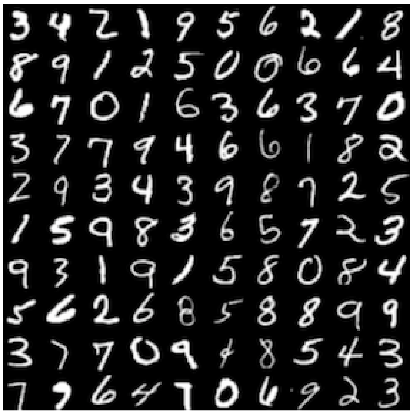
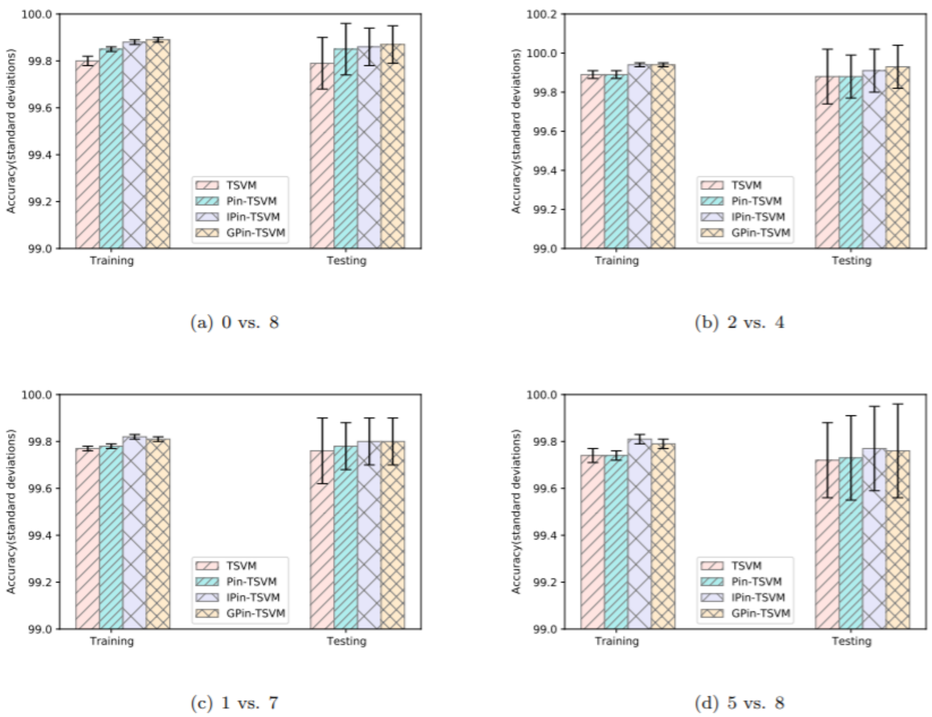
5.3. Hybrid CNN-GPin-TSVM Classifier for Handwritten Digit Recognition

The proposed algorithms GPin-TSVM and their application to handwritten digit recognition problems are discussed in this part. Handwritten digit recognition is a difficult topic that has been intensively researched in the subject of handwriting recognition for many years. As a result of its many practical uses and financial implications, handwritten digit recognition is still a popular topic. Here, we use MNIST handwritten datasets to carry out the experiments. In the field of machine learning, the MNIST dataset is commonly used for training and testing. There are 60,000 samples in the training set and 10,000 in the test set in this dataset. Each sample has a size of 28 × 28 pixels. As seen in Figure 4, the MNIST dataset comprises grayscale images of handwritten digits from ‘0’ to ‘9’. Several approaches for handwriting recognition have been proposed in the literature, such as k-nearest neighbor (KNN) [49], SVM [49,50,51,52], artificial neural network (ANN) [53,54], convolutional neural network (CNN) [51,55,56], etc.

One of the most important aspects of our cognition system success is feature extraction. Traditional feature extraction by hand is a tedious and time-consuming procedure that does not work with raw images, but features can be recovered directly from raw images using automatic extraction algorithms. On ear recognition, Alshazly [57] analyzed CNN-learnt features that are automatically optimized and found that features extracted by CNN produced the capacity to learn more specific features that are robust to wide image variations and to obtain a state-of-the-art recognition performance. On the clinical electroencephalogram (EEG) data classification problem, Xin [58] constructed a convolution support vector machine for classifying epilepsy EEG signals, and produced the highest accuracy. Recently, the hybrid CNN–SVM classifier for recognizing handwritten digits was proposed by [50,51,52]. They created a hybrid model that combines a powerful CNN with a SVM for handwritten digit recognition using the MNIST dataset, where SVM is a binary classifier and CNN is an automatic feature extractor, which both display a strong efficiency for handwritten digit recognition. Inspired by this particular work, the goal of this section is to use CNN to extract features from the MNIST dataset of input handwritten digit images. TSVM, Pin-TSVM, IPin-SVM, and GPin-TSVM work as a binary classifier, replacing the softmax layer of CNN. Moreover, we compare the performance between TSVM, Pin-TSVM, IPin-TSVM, and GPin-TSVM. We choose four pairs of handwritten digits on raw pixel features for our comparisons.

We build the network using the following. The first is placing the convolutional (Conv2D) layer into a channel of dimension 1, since the images are grayscale. The kernel size is set to $5\times 5$ with a stride of 1. This convolution output is set to nine channels, implying that it will extract nine feature maps using nine kernels. We use a padding size of 1 to ensure that the input and output dimensions are the same. These layer output dimensions are $9\times 28\times 28$. The second convolutional (Conv2D) layer has an input channel size of 9. We set the output channel size to 16, which implies that 16 feature maps will be extracted. This layer kernel size is 5 with a stride of 1. After that, we add a RelU activation and a pooling (MaxPool2D) layer with a kernel of size 2 and a stride of 2. The pooling layer is mainly integrated to reduce the data dimension. Finally, two fully connected layers are used. The first fully connected layer will receive a flattened version of the feature maps. As a result, it must have a dimension of $16\times 7\times 7$, or 256 nodes. This layer will be connected to a fully connected 80-node layer. Finally, a hidden layer of the neural network containing 84 nodes is implemented. After the architecture of the model is defined, the model needs to be compiled. Here, we use TSVM, Pin-TSVM, IPin-SVM, and GPin-TSVM, as it is a binary classification problem. The architecture of the proposed model is described in Figure 5.

We compare the performance of the proposed model on MNIST handwritten datasets with other supervised recognition systems. The results of the suggested approach on the MNIST handwritten dataset are shown in Figure 6 and the optimal parameters of the result in Figure 6 are shown in

Table 8. The optimal parameters of the result in Figure 6.

Datasets	TSVM	Pin-TSVM	IPin-TSVM	GPin-TSVM
	${\mathit{c}}_{\mathit{1}},{\mathit{c}}_{\mathit{2}}$	${\mathit{c}}_{\mathit{1}},{\mathit{c}}_{\mathit{2}},\mathit{\tau }$	${\mathit{c}}_{\mathit{1}},{\mathit{c}}_{\mathit{2}},\mathit{\tau },\mathit{ϵ}$	${\mathit{c}}_{\mathit{1}},{\mathit{c}}_{\mathit{2}},{\mathit{\tau }}_{\mathit{1}},{\mathit{\tau }}_{\mathit{2}},$ ${\mathit{ϵ}}_{\mathit{1}},{\mathit{ϵ}}_{\mathit{2}}$
0 vs. 8	0.1, 0.1	0.1, 0.1, 0.5	0.01, 0.01, 1, 1	0.01, 0.01, 1, 1, 0.1, 0.1
2 vs. 4	0.1, 0.1	0.1, 0.1, 0.5	0.1, 0.1, 1, 0.5	0.1, 0.1, 1, 1, 0.5, 0.5
1 vs. 7	1, 1	1, 1, 0.5	1, 1, 0.1, 1	1, 0.1, 1, 0.5, 0.1, 0.1
5 vs. 8	0.1, 0.1	1, 1, 1	1, 1, 0.5, 1	0.1, 0.1, 1, 0.5, 0.1, 0.5

. From Figure 6, we can learn that the classification performance of GPin-TSVM yields the best prediction accuracy of two pairwise digits out of the four total ones in terms of accuracy. On the 1 vs. 7 pairwise digit, our proposed GPin-TSVM and IPin-TSVM have an accuracy of 99.80%, which is greater than the recognition accuracy of another Pin-TSVM and TSVM classifier. However, the accuracy of GPin-TSVM on some pairwise digits, such as 5 vs. 8, is not the best. Overall, our GPin-TSVM performs well in terms of accuracy.

5.4. Statistical Analysis

On the four pairs of handwritten digits, the Friedman test is primarily used to evaluate the classification performance of the proposed GPin-TSVM algorithm. The Friedman test, along with post hoc testing, is a statistical test method that ranks algorithms differently for each data set, with the best method having the lowest ranking number [59]. The tests allow for a more accurate assessment of the algorithms’ relevance. We compare four different classifiers on four different pairs of handwritten digits. The accuracy of the related classifiers on each dataset is ranked, and the classifier with the highest accuracy has the smallest rank $r_i$. Based on the accuracy of the four pairs of handwritten digits, the average rank of all methods is shown in

Table 9. Average rank of different algorithms on four pairs of handwritten digits.

Datasets	TSVM	Pin-TSVM	IPin-TSVM	GPin-TSVM
0 vs. 8	4	3	2	1
2 vs. 4	3.5	3.5	2	1
1 vs. 7	4	3	1.5	1.5
5 vs. 8	4	3	1	2
Average Rank	3.88	3.13	1.63	1.38

.

Under the null hypothesis, the chi-square distribution and F-distribution with a degree of freedom $(k-1)(N-1)$ in the Friedman test are:

$$\begin{array}{cc}\hfill {\mathcal{X}}_F^2& =\frac{12N}{k(k+1)}\left[{\sum }_j{R}_j^2-\frac{k{(k+1)}^2}{4}\right],\\ \hfill F_F& =\frac{(N-1){\mathcal{X}}_F^2}{N(k-1)-{\mathcal{X}}_F^2},\end{array}$$

respectively, where $R_j=\frac{1}{N}{\sum }_{j=1}^N{r}_j$, the number of methods is k, and the number of datasets is N. According to Table 9, we obtain ${\mathcal{X}}_F^2=10.58$ and $F_F=22.35$. For a significance level of $0.05$, the $F(3,9)$ critical value is $3.86$, and $22.35>3.86$. As a result, the null hypothesis is rejected, i.e., there is a significant difference here between the four classifiers. Furthermore, as shown in Table 9, the proposed GPin-TSVM was ranked lowest on average. On the four pairs of handwritten digits, the classification performance of the proposed GPin-TSVM outperforms the other classifiers.

6. Conclusions

In this paper, a new version of a TSVM for pattern classification—a twin support vector machine—is created, and a generalized pinball loss function (GPin-TSVM) is implemented to improve the TSVM generalization performance, providing a lower sensitivity to noise and the ability to handle losing sparsity. We conduct wide experiments on synthetic datasets and the UCI machine learning repository, and handwritten digit recognition applications are compared to standard TSVM, Pin-TSVM, and IPin-TSVM. In most cases, the accuracy performance of our suggested GPin-TSVM is superior to that of existing classifiers, according to the experimental data. Additionally, the GPin-TSVM is less sensitive to noise and achieves sparsity, which is a major benefit of our proposed method. In the proposed GPin-TSVM, we also investigate the effect of value ${ϵ}_i(i=1,2)$. GPin-TSVM is more sparse than standard TSVM for the sparsity of the solution. At last, the proposed algorithm of GPin-TSVM was used to solve the problem of handwritten digit recognition in the application, and we used the Friedman test to evaluate the classification performance of the proposed GPin-TSVM algorithm. From the results, it can be seen that our proposed GPin-TSVM is an effective approach for handwritten digit recognition, thereby demonstrating the effectiveness of the proposed algorithm.

Our future study will focus on the applicability of GPin-TSVM to multi-class supervised classification problems and to large-scale classification problems.

References

1. Balasundaram, S.; Tanveer, M. On proximal bilateral-weighted fuzzy support vector machine classifiers. Int. J. Adv. Intell. Paradig. 2012, 4, 199–210. [Google Scholar] [CrossRef]
2. Chang, F.; Guo, C.Y.; Lin, X.R.; Lu, C.J. Tree decomposition for large-scale SVM problems. J. Mach. Learn. Res. 2010, 11, 2935–2972. [Google Scholar]
3. Zhang, C.; Tian, Y.; Deng, N. The new interpretation of support vector machines on statistical learning theory. Sci. China 2010, 53, 151–164. [Google Scholar] [CrossRef]
4. Smola, A.J.; Scholkopf, B. A tutorial on support vector regression. Stat. Comput. 2004, 14, 199–222. [Google Scholar] [CrossRef] [Green Version]
5. Tang, L.; Tian, Y.; Pardalos, P.M. A novel perspective on multiclass classification: Regular simplex support vector machine. Inf. Sci. 2019, 480, 324–338. [Google Scholar] [CrossRef]
6. van de Wolfshaar, J.; Karaaba, M.F.; Wiering, M.A. Deep Convolutional Neural Networks and Support Vector Machines for Gender Recognition. In Proceedings of the IEEE Symposium Series on Computational Intelligence, Cape Town, South Africa, 7–10 December 2015; pp. 188–195. [Google Scholar]
7. Lilleberg, J.; Zhu, Y.; Zhang, Y. Support vector machines and Word2vec for text classification with semantic features. In Proceedings of the IEEE 14th International Conference on Cognitive Informatics & Cognitive Computing (ICCI*CC), Beijing, China, 6–8 July 2015; pp. 136–140. [Google Scholar]
8. Mohammad, A.H.; Alwada’n, T.; Al-Momani, O. Arabic Text Categorization Using Support vector machine, Naïve Bayes and Neural Network. GSTF J. Comput. 2016, 5, 108–115. [Google Scholar] [CrossRef]
9. Mehmood, Z.; Mahmood, T.; Javid, M.A. Content-based image retrieval and semantic automatic image annotation based on the weighted average of triangular histograms using support vector machine. Appl. Intell. 2018, 48, 166–181. [Google Scholar] [CrossRef]
10. Richhariya, B.; Tanveer, M. EEG signal classification using universum support vector machine. Expert Syst. Appl. 2018, 106, 169–182. [Google Scholar] [CrossRef]
11. Soula, A.; Tbarki, K.; Ksantini, R.; Saida, S.B.; Lachiri, Z. A novel incremental Kernel Nonparametric SVM model (iKN-SVM) for data classification: An application to face detection. Eng. Appl. Artif. Intell. 2020, 89, 103468. [Google Scholar] [CrossRef]
12. Krishna, G.; Prakash, N. A new training approach based on ECOC-SVM for SAR image retrieval. Int. J. Intell. Enterp. 2021, 8, 492–517. [Google Scholar] [CrossRef]
13. Jayadeva; Khemchandani, R.; Chandra, S. Twin Support Vector Machines: Models; Springer: Cham, Switzerland, 2016. [Google Scholar]
14. Xu, J.; Xu, C.; Zou, B.; Tang, Y.Y.; Peng, J.; You, X. New Incremental Learning Algorithm With Support Vector Machines. IEEE Trans. Syst. 2018, 49, 2230–2241. [Google Scholar] [CrossRef]
15. Catak, F.Ö. Classification with boosting of extreme learning machine over arbitrarily partitioned data. Soft Comput. 2017, 21, 2269–2281. [Google Scholar] [CrossRef] [Green Version]
16. Jayadeva; Khemchandani, R.; Chandra, S. Twin support vector machines for pattern classification. IEEE Trans. Pattern Anal. Mach. Intell. 2007, 29, 905–910. [Google Scholar] [CrossRef] [PubMed]
17. Kumar, M.; Gopal, M. Least squares twin support vector machines for text categorization. In Proceedings of the 39th National Systems Conference (NSC), Greater Noida, India, 14–16 December 2015. [Google Scholar]
18. Francis, L.M.; Sreenath, N. Robust Scene Text Recognition: Using Manifold Regularized Twin-SupportVector Machine. J. King Saud Univ. Comput. Inf. Sci. 2007. Available online: https://www.sciencedirect.com/science/article/pii/S1319157818309509 (accessed on 2 February 2019).
19. Agarwal, S.; Tomar, D. Siddhant Prediction of software defects using Twin Support Vector Machine. In Proceedings of the International Conference on Information Systems and Computer Networks (ISCON), Mathura, India, 1–2 March 2014. [Google Scholar]
20. Cao, Y.; Ding, Z.; Xue, F.; Rong, X. An improved twin support vector machine based on multi-objective cuckoo search for software defect prediction. Int. J. Bio-Inspired Comput. 2018, 11, 282–291. [Google Scholar] [CrossRef]
21. Tomar, D.; Agarwal, S. A Multilabel Approach Using Binary Relevance and One-versus-Rest Least Squares Twin Support Vector Machine for Scene Classification. In Proceedings of the Second International Conference on Computational Intelligence & Communication Technology (CICT), Ghaziabad, India, 12–13 February 2016. [Google Scholar]
22. Gu, Z.; Zhang, Z.; Sun, J.; Li, B. Robust image recognition by L1-norm twin-projection support vector machine. Neurocomputing 2017, 223, 1–11. [Google Scholar] [CrossRef]
23. Cong, H.; Yang, C.; Pu, X. Efficient Speaker Recognition based on Multi-class Twin Support Vector Machines and GMMs. In Proceedings of the IEEE Conference on Robotics, Automation and Mechatronics, Chengdu, China, 21–24 September 2008. [Google Scholar]
24. Cumani, S.; Laface, P. Large-Scale Training of Pairwise Support Vector Machines for Speaker Recognition. IEEE/ACM Trans. Audio Speech Lang. Process. 2014, 22, 1590–1600. [Google Scholar] [CrossRef] [Green Version]
25. Nasiri, J.A.; Charkari, N.M.; Mozafari, K. Energy-based model of least squares twin Support Vector Machines for human action recognition. Signal Process. 2014, 104, 248–257. [Google Scholar] [CrossRef]
26. Sadewo, W.; Rustam, Z.; Hamidah, H.; Chusmarsyah, A.R. Pancreatic Cancer Early Detection Using Twin Support Vector Machine Based on Kernel. Symmetry 2020, 12, 667. [Google Scholar] [CrossRef] [Green Version]
27. Peng, X. TPMSVM: A novel twin parametric-margin support vector machine for pattern recognition. Pattern Recognit. 2011, 44, 2678–2692. [Google Scholar] [CrossRef]
28. Shao, Y.; Zhang, C.; Wang, X.; Deng, N. Improvements on twin support vector machines. IEEE Trans. Neural Netw. 2011, 22, 962–968. [Google Scholar] [CrossRef]
29. Shao, Y.; Chen, W.; Zhang, C.; Wang, X.; Deng, N. An efficient weighted lagrangian twin support vector machine for imbalanced data classification. Pattern Recognit. 2014, 47, 3158–3167. [Google Scholar] [CrossRef]
30. Kumar, M.A.; Gopal, M. Application of smoothing technique on twin support vector machines. Pattern Recognit. Lett. 2008, 29, 1842–1848. [Google Scholar] [CrossRef]
31. Kumar, M.A.; Khemchandani, R.; Gopal, M.; Chandra, S. Knowledge based least squares twin support vector machines. Inform. Sci. 2010, 180, 4606–4618. [Google Scholar] [CrossRef]
32. Ganaie, M.A.; Tanveer, M. LSTSVM classifier with enhanced features from pre-trained functional link network. Appl. Soft Comput. J. 2020, 93, 106305. [Google Scholar] [CrossRef]
33. Tian, Y.; Ping, Y. Large-scale linear nonparallel support vector machine solver. Neural Netw. 2014, 50, 166–174. [Google Scholar] [CrossRef]
34. Tanveer, M.; Tiwari, A.; Choudhary, R.; Jalan, S. Sparse pinball twin support vector machines. Appl. Soft Comput. J. 2019, 78, 164–175. [Google Scholar] [CrossRef]
35. Lee, Y.J.; Mangasarian, O.L. SSVM: A Smooth Support Vector Machine for Classification. Comput. Optim. Appl. 2001, 20, 5–22. [Google Scholar] [CrossRef]
36. Wu, Y.; Liu, Y. Robust truncated hinge loss support vector machines. J. Am. Stat. Assoc. 2007, 102, 974–983. [Google Scholar] [CrossRef] [Green Version]
37. Cao, L.; Shen, H. Imbalanced data classification based on hybrid resampling and twin support vector machine. Comput. Sci. Inf. Syst. 2017, 16, 1–7. [Google Scholar] [CrossRef]
38. Tomar, D.; Agarwal, S. An effective Weighted Multi-class Least Squares Twin Support Vector Machine for Imbalanced data classification. Int. J. Comput. Intell. Syst. 2015, 8, 761–778. [Google Scholar] [CrossRef] [Green Version]
39. Huang, X.; Shi, L.; Suykens, J.A.K. Support vector machine classifier with pinball loss. IEEE Trans. Pattern Anal. Mach. Intell. 2014, 36, 984–997. [Google Scholar] [CrossRef]
40. Rastogi, R.; Pal, A.; Chandra, S. Generalized pinball loss SVMs. Neurocomputing 2018, 322, 151–165. [Google Scholar] [CrossRef]
41. Mangasarian, O.L. Nonlinear Programming; Society for Industrial and Applied Mathematics: Philadelphia, PA, USA, 1994. [Google Scholar]
42. Xu, Y.; Yang, Z.; Pan, X. A novel twin support-vector machine with pinball loss. IEEE Trans. Neural Netw. Learn. Syst. 2017, 28, 359–370. [Google Scholar] [CrossRef] [PubMed]
43. Shwartz, S.; Ben-David, S. Understanding Machine Learning Theory Algorithms; Cambridge University Press: Cambridge, UK, 2014; p. 207. [Google Scholar]
44. Tikhonov, A.N.; Arsenin, V.Y. Solution of Ill Posed Problems; John Wiley and Sons: Hoboken, NJ, USA, 1977. [Google Scholar]
45. Khemchandani, R.; Jayadeva; Chandra, S. Optimal kernel selection in twin support vector machines. Optim. Lett. 2009, 3, 77–88. [Google Scholar] [CrossRef]
46. Dua, D.; Taniskidou, E.K. UCI Machine Learning Repository; University of California, School ofInformation and Computer Science: Irvine, CA, USA, 2019; Available online: http://archive.ics.uci.edu/ml (accessed on 24 September 2018).
47. Garcı, V.; Sanche, J.S.; Mollineda, R.A. On the effectiveness of preprocessing methods when dealing with different levels of class imbalance. Knowl. Based Syst. 2012, 25, 13–21. [Google Scholar] [CrossRef]
48. Hsu, C.-W.; Chang, C.-C.; Lina, C.-J. A Practical Guide to Support Vector Classification. Nat. Taiwan Univ. Taipei Taiwa 2012, 25, 1–12. [Google Scholar]
49. Hamid, N.A.; Sjarif, N.N.A. Handwritten Recognition Using SVM, KNN and Neural Network. arXiv 2017, arXiv:1702.00723. [Google Scholar]
50. Agarap, A.F.M. An Architecture Combining Convolutional Neural Network (CNN) and Support Vector Machine (SVM) for Image Classification. arXiv 2019, arXiv:1712.03541v2. [Google Scholar]
51. Ahlawata, S.; Choudhary, A. Hybrid CNN-SVM Classifier for Handwritten Digit Recognition. Procedia Comput. Sci. 2020, 167, 2554–2560. [Google Scholar] [CrossRef]
52. Aliab, A.A.A.; Mallaiah, S. Intelligent handwritten recognition using hybrid CNN architectures based-SVM classifier with dropout. Comput. Inf. Sci. 2021. [Google Scholar] [CrossRef]
53. Remaida, A.; Moumen, A.; Idrissi, Y.; El, B.; Sabri, Z. Handwriting Recognition with Artificial Neural Networks a Decade Literature Review. In Proceedings of the 3rd International Conference on Networking, Information Systems & Security, Marrakech, Morocco, 31 March–2 April 2020; pp. 1–5. [Google Scholar]
54. Aqab, S.; Tariq, M.U. Handwriting Recognition using Artificial Intelligence Neural Network and Image Processing. Int. J. Adv. Comput. Sci. Appl. 2020, 11, 137–146. [Google Scholar] [CrossRef]
55. Mawaddah, A.H.; Sari, C.A.; Setiadi, D.R.I.M.; Rachmawanto, E.H. Handwriting Recognition of Hiragana Characters using Convolutional Neural Network. In Proceedings of the International Seminar on Application for Technology of Information and Communication (iSemantic), Semarang, Indonesia, 19–20 September 2020. [Google Scholar]
56. Altwaijry, N.; Al-Turaiki, I. Arabic handwriting recognition system using convolutional neural network. Neural Comput. Appl. 2021, 33, 2249–2261. [Google Scholar] [CrossRef]
57. Alshazly, H.; Linse, C.; Barth, E.; Martinetz, T. Handcrafted versus CNN Features for Ear Recognition. Symmetry 2019, 11, 1493. [Google Scholar] [CrossRef] [Green Version]
58. Xin, Q.; Hu, S.; Liu, S.; Ma, X.; Lv, H.; Zhang, Y.D. Epilepsy EEG classification based on convolution support vector machine. J. Med. Imaging Health Inf. 2021, 11, 25–32. [Google Scholar] [CrossRef]
59. Garcia, S.; Fernandez, A.; Luengo, J.; Herrera, F. Advanced non-parametric tests for multiple comparisons in the design of experiments in computational intelligence and data mining experimental analysis of power. Inf. Sci. 2010, 180, 2044–2064. [Google Scholar] [CrossRef]
Figure 1. The workflow of the improve disadvantages of SVM.
Symmetry 14 00289 g001
Figure 2. On the 2D synthetic data, a bar graph depicting the accuracies of four algorithms.
Symmetry 14 00289 g002
Figure 3. These illustrations show the noise-insensitive features of the material. We have noise samples ranging from r = 0 % to r = 20 % . The slopes of the separating hyperplanes are indicated in brackets in the legend of each figure when we have (a) r = 0 % (free noise); (b) r = 5 ; (c) r = 10 % ; and (d) r = 20 % .
Symmetry 14 00289 g003
Figure 4. Samples from MNIST dataset.
Symmetry 14 00289 g004
Figure 5. Architecture of the CNN.
Symmetry 14 00289 g005
Figure 6. TSVM, Pin-SVM, IPin-TSVM, and GPin-TSVM accuracy and standard deviations on the MNIST dataset.
Symmetry 14 00289 g006