Rearrangement of Energy Levels between Energy Super-Bands Characterized by Second Chern Class

Abstract

We generalize the dynamical analog of the Berry geometric phase setup to the quaternionic model of Avron et al. In our dynamical quaternionic system, the fast half-integer spin subsystem interacts with a slow two-degrees-of-freedom subsystem. The model is invariant under the 1:1:2 weighted SO$\left(2\right)$ symmetry and spin inversion. There is one formal control parameter in addition to four dynamical variables of the slow subsystem. We demonstrate that the most elementary qualitative phenomenon associated with the rearrangement of the energy super-bands of our model consists of the rearrangement of one energy level between two energy superbands which takes place when the formal control parameter takes the special isolated value associated with the conical degeneracy of the semi-quantum eigenvalues. This qualitative phenomenon is of topological origin, and is characterized by the second Chern class of the associated semi-quantum system. The correspondence between the number of redistributed energy levels and the second Chern number is confirmed through a series of examples.

1. Introduction

Parametric quantum dynamical systems exhibit many different qualitative modifications under variation of his control parameters. Our purpose is to study qualitative modifications occurring in simple (molecular) quantum systems possessing slow and fast dynamical variables and one control parameter. The first step in this direction was the analysis of model Hamiltonians describing one “slow” degree of freedom (rotation) and several “fast” quantum states (vibrations) and depending on one control parameter [1]. This model exhibits a typical qualitative phenomenon, namely, the redistribution of energy levels between energy bands under the variation of the control parameter. The redistribution is associated with the formation of an isolated degeneracy point between the eigenvalues of the semi-quantum Hamiltonian which treats fast and slow variables as quantum and classical, respectively. For molecular applications of semi-quantum approach see [2,3,4,5,6,7]. The semi-quantum Hamiltonian takes the form of an Hermitian $N\times N$ matrix, with N being the number of fast quantum states taken into account, and the matrix elements being functions of the slow variables, defined over the slow classical phase space. Since the codimension of the degeneracy points of Hermitian matrices depending on parameters is three [8,9], the degeneracies of semi-quantum eigenvalues in systems with one slow degree of freedom (two dynamical parameters) and one control parameter occur generically at isolated points. It follows that the above elementary qualitative phenomenon is the dynamic version of the geometric phase setup by Berry [10,11]. The phenomenon is of topological origin and is characterized by the topological invariant [12], the first Chern class $c_1$ of the corresponding fiber bundle, with the number of redistributed energy levels being related to the topological invariants of the introduced fiber bundles [2,13,14,15].

Soon after Michael Berry formulated his geometrical phase in [10], its generalization to parametric problem with half-integer spin possessing Kramers degeneracies due to the time-reversal invariance was formulated by Mead [16] and Avron et al. [17,18]. The corresponding model Hamiltonian can be considered as a quaternionic generalization of complex Hermitian parametric Berry Hamiltonian. The construction of the dynamic quaternionic model and its analysis from the point of view of our qualitative approach treating fast (half-integer spin) states as quantum and slow dynamic variables as classical is the subject of the present note.

Due to the Kramers degeneracy of fast quantum states, the eigenvalues of the semi-quantum matrix are Kramers degenerate and the complete quantum system has degenerate bands, which we call super-bands. The eigenvalues of the semi-quantum hyperhermitian quaternionic Hamiltonian have codimension 5 degeneracies and consequently, the simplest model with qualitative modifications of the super-band structure could appear for at least four fast states (two Kramers degenerate pairs), a slow subsystem of two degrees of freedom (four classical variables), and one control parameter. The topological invariant associated with the formation of the codimension 5 degeneracy is now the second Chern class [19]. As in [1] we conjecture that this class corresponds to the number of quantum energy levels redistributed between the super-bands under the variation of the control parameter. The redistribution is associated with the specific isolated parameter value, for which two degenerate pairs of semi-quantum eigenvalues form a four-fold degeneracy point.

Without going into strict mathematical details associated with the definition of the spectral flow in the context of the Atiyah–Singer theorem [20,21,22] we show on concrete examples that typical qualitative modifications of the (super)band structure can be interpreted in terms of the correspondence between semi-quantum and quantum quaternionic Hamiltonians and allows to relate topological invariant associated with formation of degeneracy point for semi-quantum model to the number of redistributed quantum energy levels.

2. Model Construction

We begin by reviewing the qualitative analysis of model Hamiltonians describing interaction of two “fast” quantum states with one “slow” degree of freedom. The spin operators $(S_1,S_2,S_3)$ with ${\mathbf{S}}^2=3/4$ describe the fast subsystem. The slow subsystem is described by angular momentum components $(N_1,N_2,N_3)$, satisfying $N_1^2+N_2^2+N_3^2=const$. The operator form of the model quantum Hamiltonian takes the form

$$\begin{array}{c}\hfill H=cos\alpha S_1+sin\alpha \mathbf{S}·\mathbf{N},\end{array}$$

(1)

where $\alpha$ is the control parameter, whose variation we restrict to the domain $0\le \alpha \le \pi$. Due to the axial symmetry of the system, the quantum version of Hamiltonian (1) possesses explicit solutions for eigenvalues and eigenfunctions [1]. The secular equation decomposes into several quadratic, and two linear equations for eigenvalues. For any fixed value of quantum number N, the eigenvalue of the operator ${\mathbf{N}}^2$ equals $N(N+1)$, and the energy level pattern consists of $2(2N+1)$ quantum energy levels forming for $\alpha \sim 0$ and $\alpha \sim \pi$ two well separated and almost degenerate energy bands consisting of $2N+1$ energy levels each. Near the control parameter value $\alpha \sim \pi /2$, two nearly degenerate energy bands also exist, but now the number of the energy levels in these bands is different: the upper-in-energy band consists of $2N+2$ quantum levels, while the lower-in-energy band consists of $2N$ levels. Schematic representation of the quantum energy level pattern for the Hamiltonian (1) is shown in Figure 1 in the form of correlation diagram relating $\alpha =0,\pi /2,\pi$ limiting cases.

The two bands at the $\alpha =0$ and $\alpha =\pi$ endpoints correspond to the uncoupled system, and the global evolution of the pattern of energy levels under the variation of $\alpha$ between $\alpha =0$ and $\alpha =\pi$ can be interpreted as crossover of the band structure going through the intermediate system with coupled spin and orbital momentum at $\alpha \sim \pi /2$. The two bands near $\alpha =\pi /2$ are characterized by the total angular momentum quantum number $J=N+1/2$ and $J=N-1/2$.

As can be seen in Figure 1, the rearrangement of the energy levels between the energy bands is associated with the transition of two quantum levels with $J_1=N+1/2$ and $J_1=-N-1/2$. To see the topological origin of the rearrangement phenomenon, we construct the semi-quantum model by replacing slow quantum operators by classical variables. In the basis of $|S_1=\pm \frac{1}{2}\rangle$ functions, this results in the $2\times 2$ Hermitian matrix

$$\begin{array}{c}\hfill H_{semi-q}=\left(\begin{array}{cc}\frac{1}{2}cos\alpha +\frac{1}{2}sin\alpha N_1& \frac{1}{2}sin\alpha N_{-}\\ \frac{1}{2}sin\alpha N_{+}& -\frac{1}{2}cos\alpha -\frac{1}{2}sin\alpha N_1\end{array}\right)\end{array}$$

(2)

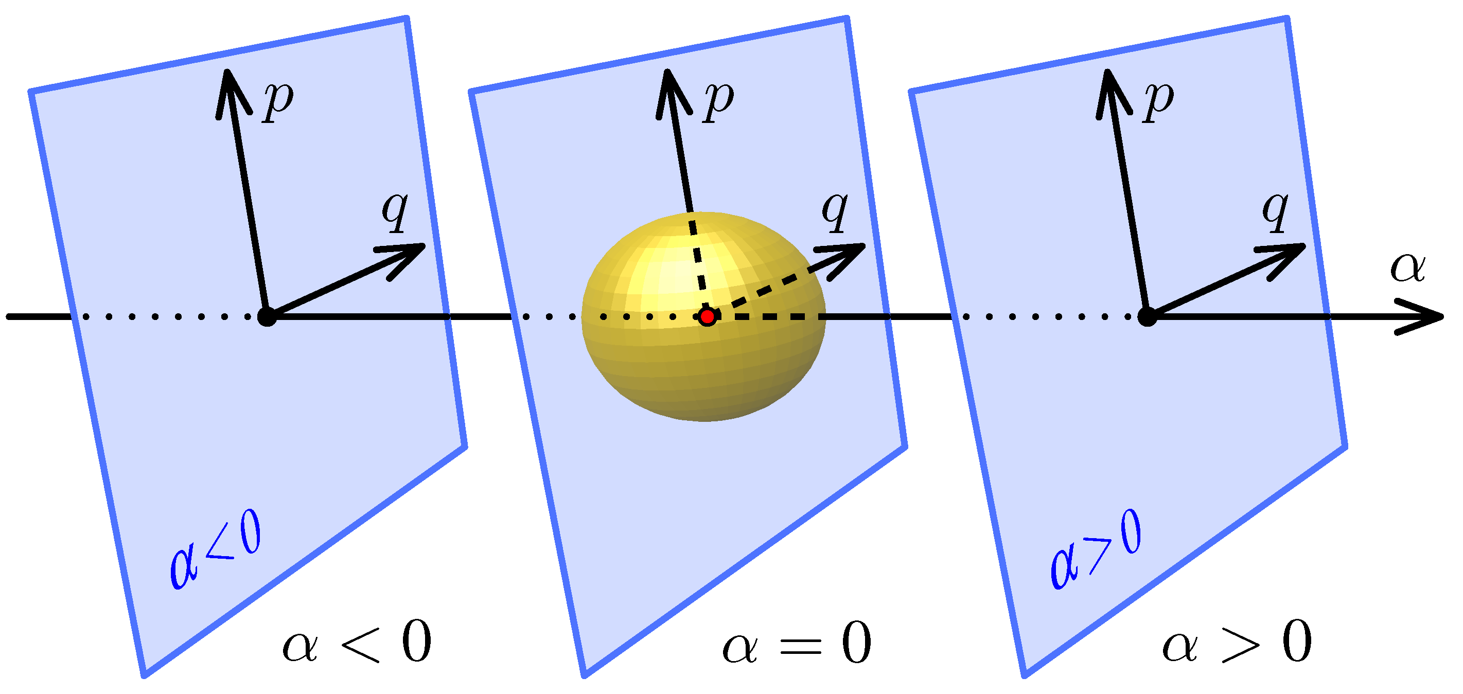
The eigenvalues of the above semi-quantum matrix Hamiltonian become degenerate at the isolated points of the three-dimensional space $\{P,\alpha \}$, where P is the two-dimensional classical phase space for slow subsystem and $\alpha$ is the control parameter. More specifically, P is a two-dimensional sphere $S^2$, defined by $N_1^2+N_2^2+N_3^2=N^2$.

The complex eigenfunctions of semi-quantum Hamiltonian (2) form a rank-two fiber bundle which can be decomposed into two line eigenbundles if the eigenvalues are not degenerate. The degeneracy of two eigenvalues of semi-quantum Hamiltonian occurs at isolated points of the three-dimensional base space $(P,\alpha )$: $\{N_1=N,N_2=N_3=0,\alpha =\pi /4\}$ and $\{N_1=-N,N_2=N_3=0,\alpha =3\pi /4\}$.

These line eigenbundles can be characterized topologically in two slightly different ways. We can consider eigenbundle defined on the closed regular spherical surface in the three-dimensional $\{P,\alpha \}$ space surrounding the degeneracy point $\{P_{\mathrm{deg}},{\alpha }_{\mathrm{deg}}\}$ of the semi-quantum eigenvalues. We denote this bundle ${\Delta }_k(P_{\mathrm{deg}},{\alpha }_{\mathrm{deg}})$. Its construction reproduces the one suggested by Simon [12] and used by Mead [16] and Avron et al. [17,18]. Alternatively, we can consider the fiber bundle with the base space being the classical phase space P of the slow subsystem for fixed value of control parameter $\alpha$. When there is no degeneracy of eigenvalues, each line eigenbundle is characterized by the first Chern class $c_1$. We denote such eigenbundle by ${\Lambda }_k\left(\alpha \right)$. The topological invariant $c_1$ for ${\Lambda }_k\left(\alpha \right)$ is a piece-wise constant function of control parameter $\alpha$ which is not defined for the special parameter values $\alpha ={\alpha }_{\mathrm{deg}}$ corresponding to the degeneracies of the semi-quantum eigenvalues. The topological invariant $c_1$ of the ${\Delta }_k(P_{\mathrm{deg}},{\alpha }_{\mathrm{deg}})$ bundle plays the role of “$\delta$-Chern” for the $c_1$ invariant for the ${\Lambda }_k\left(\alpha \right)$ bundle. It gives the jump of $c_1\left({\Lambda }_k\left(\alpha \right)\right)$ that occurs when the control parameter $\alpha$ passes the special isolated values ${\alpha }_{\mathrm{deg}}$ corresponding to the degeneracy of semi-quantum eigenvalues (we assume for simplicity that there is only one degeneracy point $(P_{\mathrm{deg}},{\alpha }_{\mathrm{deg}})$ for any ${\alpha }_{\mathrm{deg}}$) [2,13,14,15]. The base spaces of $\Delta$ and $\Lambda$ bundles are represented schematically in Figure 2.

It is important to note that topological invariants $c_1\left({\Delta }_k\right)$ for the semi-quantum version of Hamiltonian (1) are well defined (over the sphere surrounding the degeneracy point) regardless on whether the slow classical phase space P is compact or not [15]. On the other hand, $c_1\left({\Lambda }_k\right)$ can be defined for any $0\le \alpha \ne \pi /2\pm \pi /4\le 1$ because the classical phase space for slow variables is compact. Only formal Chern numbers can be used for problems with non-compact space of slow variables [23,24].

Comparing the topological modifications of the semi-quantum eigenfunction bundles to the evolution of the energy spectrum of the parent quantum system, we find that the number of redistributed quantum energy levels equals (with appropriate choice of the sign) the Chern numbers $c_1\left({\Delta }_k(P_{\mathrm{deg}},{\alpha }_{\mathrm{deg}})\right)$ associated with the corresponding degeneracy point of the semi-quantum eigenvalues. 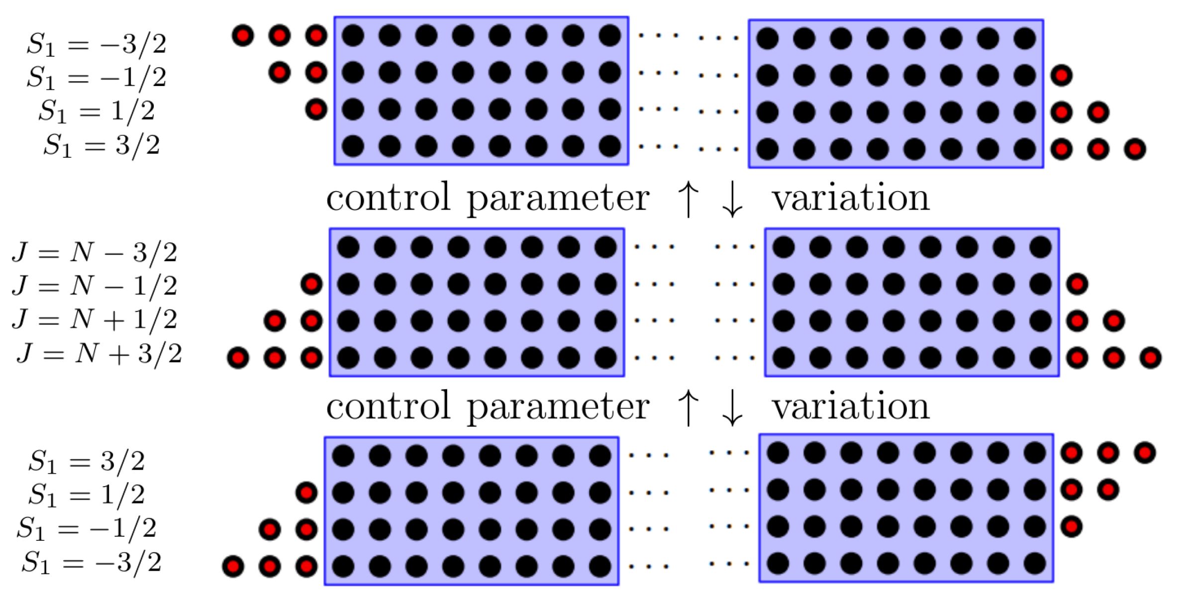Figure 3 illustrates schematically the rearrangement of the set of basis functions describing the two bands of the spin-$\frac{1}{2}$ axially symmetric model system. The basis functions are classified according to their axial symmetry and describe the “edge” states (with $J_1=\pm (J+1/2)$) belonging to different bands at various values of control parameter and “bulk” states (with $-J+1/2\le J_1\le J-1/2$) belonging to the same band at all different regular values of control parameter. The most simple generic qualitative modification of the energy bands in the slow-fast system with one slow degree of freedom consists of the jump of the first Chern class $\delta c_1=\pm 1$ of the semi-quantum system and in the redistribution of the single quantum level between two energy bands in the corresponding quantum system. In the case of additional symmetries, the concepts of local delta-Chern and of the orbit of degeneracy points should be properly introduced and applied [14,15]. For $S=1/2$, the model Hamiltonian (1) has two degeneracy points of semi-quantum eigenvalues occurring at the north and south poles of the classical phase space $P={\mathbb{S}}^2$ (which we denote by $(+)$ and $(-)$, respectively) at two different isolated values of control parameter. The associated redistribution of the edge energy levels is represented in Figure 3 as the modification of the set of basis functions associated with each band under the control parameter variation. Extension to arbitrary spin $S>\frac{1}{2}$ does not change the number of degeneracy points of Hamiltonian (1) but results in more complicated simultaneous degeneracy of all $2S+1$ bands. Splitting the basis set into the edge and bulk states for the case of $S=\frac{3}{2}$ is represented in Figure 4. From this figure, we can derive easily the number of lost/gained energy levels for each of the $2S+1$ bands of the system after the critical control parameter value associated with the isolated degeneracy is crossed. For the band attributed in the uncoupled limit to a particular fixed value of $k=S_1$, the number of the lost/gained levels equals (depending on the direction of the assumed control parameter evolution) $\pm 2S_1$. At the same time, this number equals (to a sign convention) the first Chern number $c_1\left({\Delta }_k(P_{\mathrm{deg}},{\alpha }_{\mathrm{deg}})\right)$ of the corresponding line eigenbundle component defined over the 2-sphere surrounding the degeneracy point $(P_{\mathrm{deg}},{\alpha }_{\mathrm{deg}})$ (yellow sphere in Figure 2 surrounding the red point).

The above discussion summarizes briefly the principal results of the qualitative analysis of complex generic Hamiltonians describing quantum systems formed by fast subsystem (of several quantum states) and slow subsystem (with one degree of freedom) and depending on one control parameter. This analysis can be regarded as a dynamic realization [1] of the geometric phase setup by Berry [10]. In the present paper we want to formulate the generalization of this dynamic construction for the non-Abelian geometric phase setup of Mead [16] and Avron et al. [17,18].

The basic physical idea behind this generalization is to study qualitative modifications of the energy band spectrum in systems consisting of coupled fast and slow subsystems, but whose fast subsystem is characterized by half-integer spin and is invariant under spin reversal [25,26]. The invariance of the fast subsystem under the spin reversal is equivalent for the parametric model of Avron et al. to time reversal invariance because there is no other dynamical variables. Spin reversal results in the so-called quaternionic form of the semi-quantum Hamiltonian with all eigenvalues being Kramers (doubly) degenerate [27,28]. Due to the Kramers degeneracy of the semi-quantum eigenvalues of the fast subsystem, we should treat the two components of the Kramers doublets together and should analyze super-bands or doublet-bands rather than simple bands. The codimension of the degeneracy of two Kramers-degenerate pairs of eigenvalues of generic quaternionic semi-quantum Hamiltonians is five. Consequently, the generic qualitative modification of the band structure in quaternionic dynamical systems can occur if such systems possess two slow degrees of freedom providing four dynamical variables in addition to one formal control parameter. In such a case, under variation of the formal control parameter, an isolated degeneracy point of two Kramers-degenerate doublets can be formed generically and can be associated with the redistribution of energy levels between superbands in the quantum version of the same system. Due to the double degeneracy of all quaternionic semi-quantum eigenvalues, the fibre bundles formed by the respective eigenfunctions are generically (in the absence of additional degeneracies of eigenvalues) of rank two, and should be characterized by the second Chern class $c_2$ [29].

The qualitative analysis of corresponding quantum Hamiltonians shows that the formation of isolated degeneracy points of semi-quantum eigenvalues corresponds to the rearrangement of energy levels between superbands. In the most trivial generic situation, this rearrangement involves the transfer of one quantum energy level. Conjecturally, the number of quantum levels which are redistributed under the variation of control parameter $\alpha$ across the degeneracy point ${\alpha }_{\mathrm{deg}}$ to/from the k-th band in the spectrum of the quantum quaternionic Hamiltonian corresponds to the second Chern class $c_2\left({\Delta }_k\left({\alpha }_{\mathrm{deg}}\right)\right)$ computed for the corresponding semi-quantum Hamiltonian. We confirm this conjecture on the examples below.

We begin by choosing the slow and fast dynamic variables needed to construct our model quantum Hamiltonian. The fast subsystem is described by spin operators $(S_1,S_2,S_3)=\mathbf{S}$ with fixed value of ${\mathbf{S}}^2=S(S+1)$. We take $S=3/2$ to model the simplest interesting situation with redistribution of quantum energy levels between two Kramers doublets (two superbands). The slow subsystem is described by angular momentum operators $\mathbf{X}=(X_1,X_2,X_3)$ and $\mathbf{Y}=(Y_1,Y_2,Y_3)$ with fixed norms ${\mathbf{X}}^2=X(X+1)$, ${\mathbf{Y}}^2=Y(Y+1)$. These angular momenta commute with each other and with spin $\mathbf{S}$. The Hamiltonian is supposed (by construction) to be invariant with respect to the weighted action of the SO(2) group. The action on dynamic variables ${\omega }_S:{\omega }_X:{\omega }_Y=1:1:2$ is given as follows. Note that weighted action $1:1:(-2)$ which will be mentioned below leads to slightly different results.

$$\begin{array}{cc}\hfill & R\left(\phi \right)\left(S_1,S_{+},S_{-}\right)\to \left(S_1,exp\left(i\phi \right)S_{+},exp(-i\phi )S_{-}\right),\end{array}$$

(3)

$$\begin{array}{cc}& R\left(\phi \right)\left(X_1,X_{+},X_{-}\right)\to \left(X_1,exp\left(i\phi \right)X_{+},exp(-i\phi )X_{-}\right),\end{array}$$

(4)

$$\begin{array}{cc}& R\left(\phi \right)\left(Y_1,Y_{+},Y_{-}\right)\to \left(Y_1,exp\left(2i\phi \right)Y_{+},exp(-2i\phi )Y_{-}\right),\end{array}$$

(5)

where we use the notation $A_{\pm }=A_2\pm A_3$ for $A=S,X,Y$.

Due to presence of this weighted SO(2) symmetry, there exists the integral of motion

$$\begin{array}{c}\hfill j_1=S_1+X_1+2Y_1.\end{array}$$

(6)

Another a priori symmetry requirement is the invariance with respect to the inversion of the sign of the $\mathbf{S}$ components. We denote this operation, which acts only on spin, by ${\mathcal{T}}_S$

$$\begin{array}{c}\hfill {\mathcal{T}}_S\mathbf{S}=-\mathbf{S},{\mathcal{T}}_S\mathbf{X}=\mathbf{X},{\mathcal{T}}_S\mathbf{Y}=\mathbf{Y}.\end{array}$$

(7)

The invariance with respect to ${\mathcal{T}}_S$ implies that the Hamiltonian should be of even degree (at least quadratic) in $S_k$.

In what follows we consider S to be half-integer and $X,Y$ to be integer and satisfying $X,Y\gg S$. This requirement is based on the assumption that $\mathbf{S}$ describes fast quantum subsystem, whereas $\mathbf{X}$ and $\mathbf{Y}$ describe the slow classical subsystem.

2.1. Quantum Model Hamiltonian

In order to generalize Hamiltonian (1) to describe systems with two slow degrees of freedom, half-integer spin S, and Kramers degeneracy for semi-quantum eigenvalues, we consider the following low-degree contributions invariant with respect to SO$\left(2\right)$ and ${\mathcal{T}}_{\mathcal{S}}$ symmetry.

The terms which are diagonal in $S_1$ include the traceless term

$$\begin{array}{c}\hfill S_1^2-{\mathbf{S}}^2/3,\end{array}$$

(8a)

which describes splitting of the entire set of basis functions into subsets with $|S_1|=\frac{1}{2},\frac{3}{2},\dots$. This term replaces the first term in (1), but contrary to its predecessor, it is invariant with respect to both ${\mathcal{T}}_S$ and complete time reversal. When this term is dominant (and all other contributions are negligible), there exist well-separated superbands characterized by $|S_1|$. For $S=3/2$ there are two superbands with $S_1=\pm \frac{3}{2}$ and $S_1=\pm \frac{1}{2}$. Inversion of the sign of (8a) results in the crossover (inversion of energy) of the superband spectrum. The two other diagonal terms

$$X_1(S_1^2-S^2/3)\mathrm{and}{Y}_1(S_1^2-S^2/3)$$

(8b)

represent the diagonal part of the spin–orbital interaction. They are invariant only with respect to ${\mathcal{T}}_S$.

The contributions which are non-diagonal in $S_1$ include

$$X_{\pm }\left(S_1{S}_{\mp }+S_{\mp }{S}_1\right)\mathrm{and}{Y}_{\pm }{S}_{\mp }^2.$$

(8c)

Like (8b), these terms are ${\mathcal{T}}_s$-invariant, but they are not invariant with respect to the complete time reversal. Note that transformation properties of dynamical variables under SO$\left(2\right)$ symmetry group

$$\begin{array}{cccc}\hfill \begin{array}{c}\hfill \mathrm{SO}\left(2\right)\mathrm{irrep}\end{array}& 0& \pm 1\hfill & \pm 2\\ \hfill \mathrm{Terms}& S_1,X_1,Y_1& S_{\pm },X_{\pm }\hfill & S_{\pm }^2,Y_{\pm }\end{array}$$

(9)

mean that the first of (8c) terms represents the $1:1$ resonance between the fast spin subsystem and slow X-subsystem, while the second term in (8c) corresponds to the $1:2$ resonance of spin and Y subsystem. It follows that by construction, any combination of (8c) represents the $1:1:2$ fast-slow resonance. Further observe that the presence of the anticommutator $S_1{S}_{\mp }+S_{\mp }{S}_1$ results in the zero value of the non-diagonal block $\langle S_1=\pm \frac{1}{2}|\dots |S_1=\mp \frac{1}{2}\rangle$. This is required for the semi-quantum matrix to be quaternionic.

Collecting all terms in (8), the quantum Hamiltonian takes the following form

$$\begin{array}{ccc}\hfill H_q& =& \alpha \left(S_1^2-\frac{S^2}{3}\right)+d_{1q}{X}_1\left(S_1^2-\frac{S^2}{3}\right)+d_{2q}{Y}_1\left(S_1^2-\frac{S^2}{3}\right)\hfill \\ & +& c_{1q}\left(X_{+}\left(S_1{S}_{-}+S_{-}{S}_1\right)+X_{-}\left(S_1{S}_{+}+S_{+}{S}_1\right)\right)+c_{2q}\left(Y_{+}{S}_{-}^2+Y_{-}{S}_{+}^2\right)\hfill \end{array}$$

(10)

with real coefficients. The coefficients $c_{iq},d_{iq}$ are supposed to be fixed, whereas $\alpha$ is considered a control parameter responsible for the crossover of the band structure. Note that parameter $\alpha$ plays the role of $sin\alpha ,cos\alpha$ terms in (1).

The eigenfunctions of the Hamiltonian (10) can be written as the superposition of the uncoupled-basis functions

$$\begin{array}{c}\hfill {\Psi }_n=\sum _{m_S,m_X,m_Y}{c}_{m_S,m_X,m_Y}\left|S,m_S;X,m_X;Y,m_Y\right.〉.\end{array}$$

(11)

To be more concrete, we consider the case $S=\frac{3}{2}$. The Hamiltonian (10) has two obvious limits which correspond to $\alpha \to \pm \infty$. In each of these trivial limits, all energy levels are grouped into two superbands, one with positive energy, the other with negative energy. One superband includes all eigenstates with $m_S=\pm \frac{3}{2}$, while the other consists of the eigenstates with $m_S=\pm \frac{1}{2}$.

2.2. Generating Functions for Numbers of States

The number of states in the two superbands in both trivial limiting cases is the same but the distribution of eigenstates with respect to the integral $j_1$ (6) is superband specific and depends on the value of the control parameter $\alpha$. This means that when $\alpha$ is varied, an exchange of energy levels between the two superbands must take place.

To characterize the redistribution of quantum energy levels between trivial limit superbands with different $|S_1|$ under the variation of the crossover control parameter, it is useful to construct the correlation diagram which takes into account the classification of quantum energy levels by the $1:1:2$ symmetry, i.e., by the conserved value of $j_1$. We use for this purpose generating functions [30].

The generating function for the number of states with the same value of $j_1$ for the entire problem with arbitrary positive integer X, Y, and half-integer S is

$$\begin{array}{c}\hfill g^{1:1:2}\left(t\right)=\frac{\left(1-t^{2S+1}\right)\left(1-t^{2X+1}\right)\left(1-t^{2(2Y+1)}\right)}{{(1-t)}^2(1-t^2)}=\sum _{n=0}{C}_n{t}^n.\end{array}$$

(12)

The coefficient $C_n$ in the Taylor series expansion of the generating function gives the number of states with given $j_1=n-(X+2Y+S)$.

In order to count the number of states with given $j_1$ belonging separately to one of the superbands with given projection $|S_1|=\sigma$ (in the limit of $\alpha \to \pm \infty$ where such superbands are well defined), we transform the generating function (12) into the following form

$$\begin{array}{c}\hfill g^{1_{\sigma }:1:2}\left(t\right)=\frac{\left(t^{S-\sigma }+t^{S+\sigma }\right)\left(1-t^{2X+1}\right)\left(1-t^{2(2Y+1)}\right)}{(1-t)(1-t^2)}=\sum _{n=0}{C}_{n,\sigma }{t}^n.\end{array}$$

(13)

The term $C_{n,\sigma }{t}^n$ in the Taylor expansion of (13) means that among all basis functions (states) with $j_1=n-(S+X+2Y)$ there are $C_{n,\sigma }$ functions (states) with $S_1=\pm \sigma$.

We consider the case of $S=\frac{3}{2}$ (Figure 5) with two superbands in more detail. The energies of these superbands are inversed in the limits of $\alpha \to \pm \infty$. In other words, when the control parameter $\alpha$ is varied from $-\infty$ to $+\infty$, the superband structure “crosses over”. This does not mean that all states of the upper band go down and all states of the lower band go up. Quite the opposite (Figure 5), similarly to the spin–orbit system with Hamiltonians (1)–(2), most of the states, called “bulk”, remain within their superbands, while only a few states, called “edge”, need to be transferred between the superbands. Using generating function (13), we can obtain the explicit expressions for the number of the eigenfunctions $|j_1\rangle$, which are exchanged in the crossover. For $S=\frac{3}{2}$, the difference of generating functions in the two limiting cases gives

$$\begin{array}{c}\hfill \frac{\left(1+t^3-t-t^2\right)\left(1-t^{2X+1}\right)\left(1-t^{2(2Y+1)}\right)}{(1-t)(1-t^2)}=1-t^{4Y+2}-t^{2X+1}+t^{2X+3+4Y}.\end{array}$$

(14)

The coefficient at $t^n$ gives the number of the edge quantum states with

$$j_1=n-j_{\max }=n-\left(X+2Y+\frac{3}{2}\right)$$

and the direction of their redistribution. We conclude that during the crossover of the spin-$\frac{3}{2}$ superband structure, four quantum states must be tranferred between the superbands. As illustrated in Figure 5, two quantum states with extremal values $j_1=\pm (X+2Y+3/2)$ move in one direction, while two other states with $j_1=\pm (X-2Y-1/2)$ go in the opposite direction. However, the correlation diagram does not reproduce the order (as function of $\alpha$) in which quantum levels are redistributed between limiting cases.

Consider now the total number $n\left(k\right)$ of the slow subsystem basis wavefunctions $\left|k\right(X_1,Y_1)\rangle$ which are eigenfunctions of $K=X_1+2Y_1$, the momentum of the slow $1:2$-resonant SO(2) symmetry, with eigenvalue k, and the number $n_{S_1}\left(j_1\right)$ of slow-fast basis functions $|S_1\rangle |k(X_1,Y_1)\rangle$ for each spin basis component with $S_1=-S,-S+1,\dots ,S-1,S$ as function of the integral of motion $j_1$ in (6). We say that these functions give, respectively, the slow and the $S_1$-specific slow-fast distributions of basis wavefunctions. Note that $n_{S_1}\left(j_1\right)$ follows from $n\left(k\right)$ after a trivial linear shift of its argument k by $S_1$, so that $n_{S_1}\left(j_1\right)=n_{S_1^{\prime }}(j_1+S_1^{\prime }-S_1)$. Quantum distribution $n\left(k\right)$ is a piecewise function which combines a linear staircase-function and, depending on the relative values of X and $2Y$, a step-function or a constant function [30]. In the classical limit of large X and Y, we can ignore the ℏ-small steps and approximate the distribution $n\left(k\right)$ by the Duistermaat–Heckman diagram [31] representing the volume of the reduced slow phase space $P_k$ as function of the value k of momentum K. 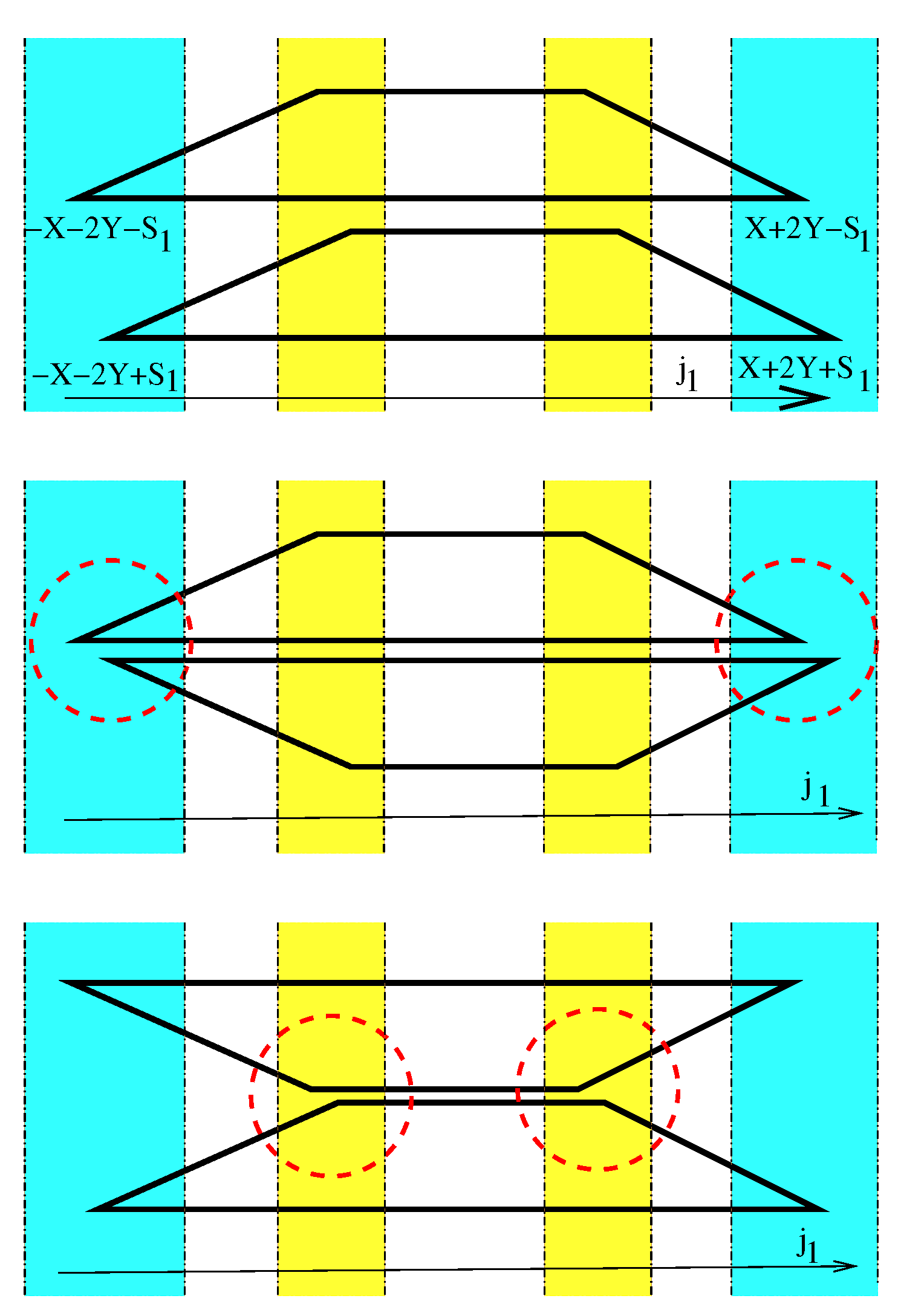By the Duistermaat–Heckman theorem, since the total slow phase space $P={\mathbb{S}}^2\times {\mathbb{S}}^2$ and the reduced spaces $P_k$ are of respective dimensions 4 and 2, this diagram is piece-wise linear, and it can be further argued, that in our case, it is symmetric with respect to $k\to -k$, and has the form of a trapezoid. Shifting for each $S_1$ components as shown in Figure 6, we obtain similar diagrams $n_{S_1}\left(j_1\right)$ for each $S_1$ component of each superband $|S_1|$. In particular, it can be seen that the number-of-state function for superband $|S_1|$ is a sum of two distributions $n_{\pm |S_1|}\left(j_1\right)$, which are shifted one with respect to another by $2|S_1|$. It becomes clear that the difference in the number-of-state function for different superbands is localized in the four regions near $j_1$ values corresponding to the vertices of the diagram with $|S_1|=\frac{1}{2}$. In order to visualize better the number-of-state function for superbands, we join the distributions $n_{\pm |S_1|}\left(j_1\right)$ in two alternative graphical ways, as depicted in Figure 6, middle and bottom, where the parts that are important to further analysis are marked by red dashed circles.

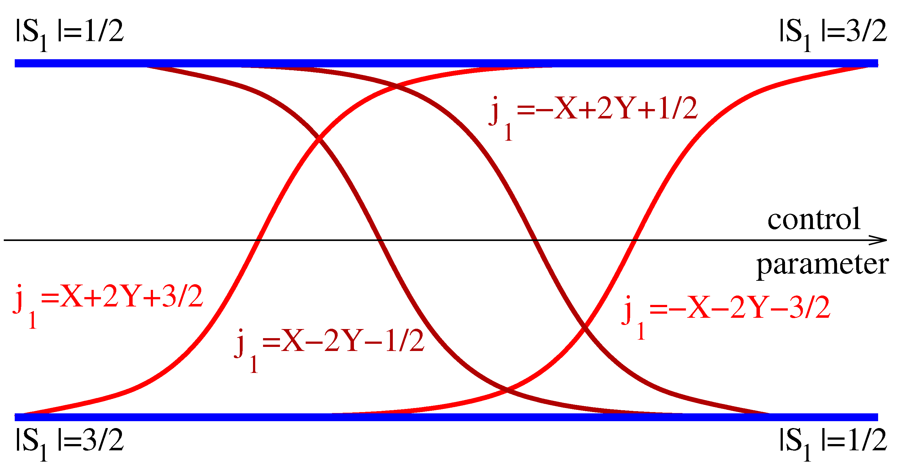
Before going further into the local analysis of the number-of-states functions in the case of arbitrary S, we would like to return to the quantum system with $S=3/2$. According to our general conjecture, the distribution of energy levels between energy (super)bands can be realized at control parameter values associated with the formation of degeneracy points between the eigenvalues of the semi-quantum version of the quantum Hamiltonian. The latter is obtained from (10) by replacing angular momentum operators $\widehat{\mathbf{X}}$ and $\widehat{\mathbf{Y}}$ by their classical analogs and computing matrix elements of the spin operators in the basis $\left\{\right|S_1=3/2\rangle ,|S_1=-3/2\rangle ,|S_1=-1/2\rangle ,|S_1=1/2\rangle \}$. We obtain the $4\times 4$ matrix

$$\begin{array}{c}\hfill \left(\begin{array}{cccc}\alpha +d_{1q}{X}_1+d_{2q}{Y}_1& 0& c_{2q}\sqrt{6}{Y}_{-}& c_{1q}2\sqrt{3}{X}_{-}\\ 0& \alpha +d_{1q}{X}_1+d_{2q}{Y}_1& -c_{1q}2\sqrt{3}{X}_{+}& c_{2q}\sqrt{6}{Y}_{+}\\ c_{2q}\sqrt{6}{Y}_{+}& -c_{1q}2\sqrt{3}{X}_{-}& -\alpha -d_{1q}{X}_1-d_{2q}{Y}_1& 0\\ c_{1q}2\sqrt{3}{X}_{+}& c_{2q}\sqrt{6}{Y}_{-}& 0& -\alpha -d_{1q}{X}_1-d_{2q}{Y}_1\end{array}\right),\end{array}$$

(15)

where $X_1,X_{\pm },Y_1,Y_{\pm }$ are components of classical angular momenta, $d_{1q},d_{2,q},c_{1q}.c_{2q}$ are fixed real phenomenological coefficients of model Hamiltonian (10) and $\alpha$ is a control parameter. Rewriting this matrix in a more symbolic form

$$\begin{array}{c}\hfill \left(\begin{array}{cccc}t& 0& a+ib& c+id\\ 0& t& -c+id& a-ib\\ a-ib& -c-id& -t& 0\\ c-id& a+ib& 0& -t\end{array}\right),\end{array}$$

(16)

we can see that it is of the typical quaternionic form with real coefficients $a,b,c,d,t$ and consequently, the semi-quantum Hamiltonian (16) has two doubly degenerate eigenvalues. Their explicit analytical expression $E_{1,2;3,4}=\pm \sqrt{a^2+b^2+c^2+d^2+t^2}$ shows that the degeneracy of eigenvalues occurs only if the five conditions are satisfied $a^2=b^2=c^2=d^2=t^2=0$. This provides an elementary demonstration of the codimension 5 degeneracy of the eigenvalues of the quaternionic hyper-Hermitian matrix. These eigenvalues depend on five parameters, which include four dynamical parameters being local coordinates on the slow classical phase space $P=S^2\times S^2$, and one formal parameter $\alpha$ describing the crossover of the superband structure. Their isolated degeneracies can be easily found because they are associated with fixed points (critical orbits) of the SO(2) group action on P.

The action of the $1:2$ weighted SO(2) symmetry group on the slow classical phase space $S^2\times S^2$

$$\begin{array}{c}\hfill R\left(\phi \right)\left({\theta }_X,{\varphi }_X,{\theta }_Y,{\varphi }_Y\right))\to \left({\theta }_X,{\varphi }_X+\phi ,{\theta }_Y,{\varphi }_Y+2\phi \right),\end{array}$$

(17)

expressed here in terms of spherical coordinates on each of the $S^2$ factors in $S^2\times S^2$, has four isolated critical one-point orbits, the poles at which $X_1=\pm X$ and $Y_1=\pm Y$, and which can be denoted accordingly as $(++)$, $(+-)$, $(-+)$, and $(--)$.

$$\begin{array}{cc}\hfill & (++):(X_1=X,Y_1=Y);(--):(X_1=-X,Y_1=-Y);\end{array}$$

(18a)

$$\begin{array}{cc}& (+-):(X_1=X,Y_1=-Y);(-+):(X_1=-X,Y_1=Y).\end{array}$$

(18b)

Four values of control parameter $\alpha$ at which degeneracy points of semi-quantum version of quantum Hamiltonian (10) occur are

$${\alpha }_{\mathrm{deg}}=\pm \left(d_{1q}X\pm d_{2q}Y\right),$$

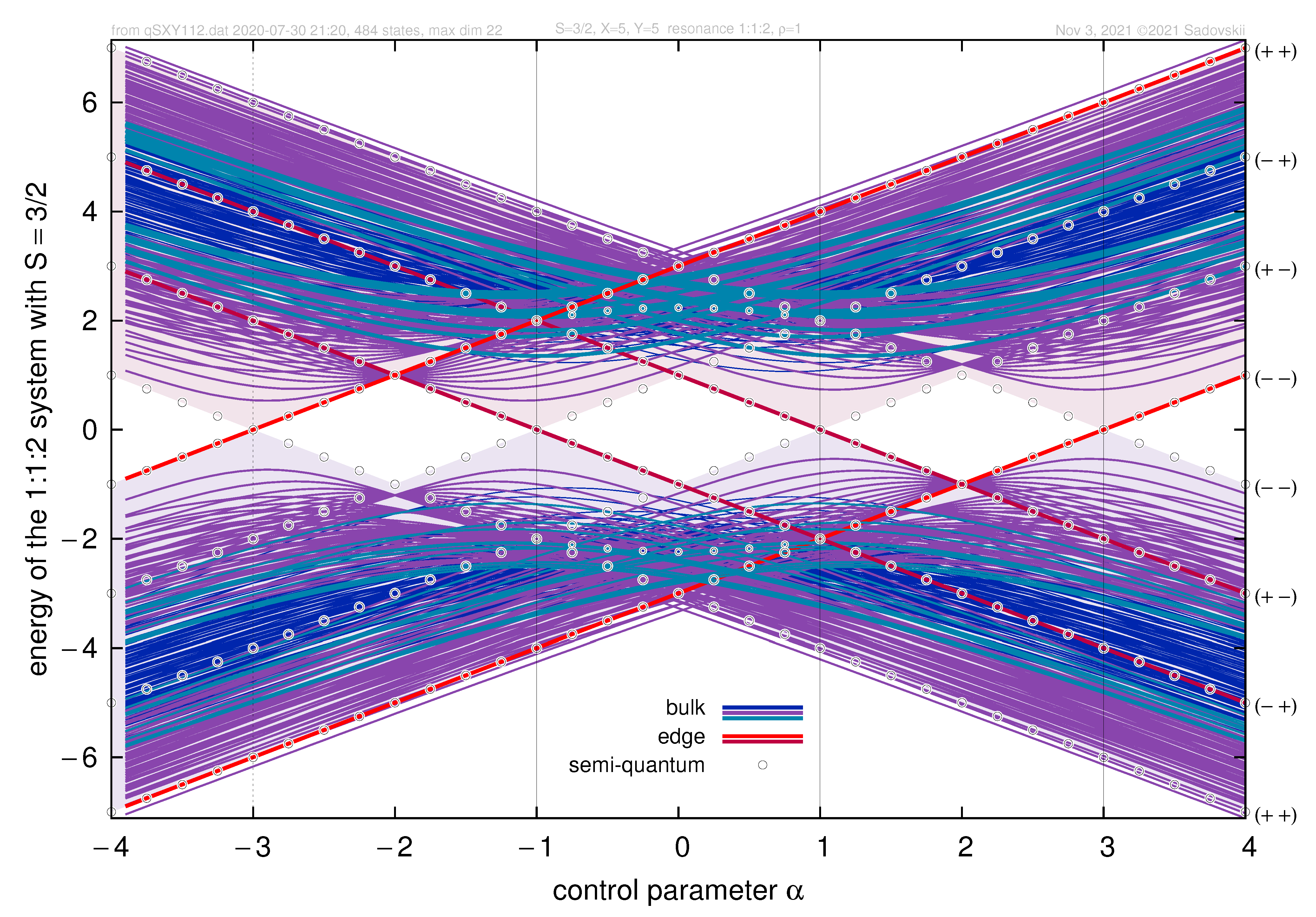
Each of the four conical degeneracy points is associated with the transfer of a single quantum level between the two superbands. This is illustrated by the results of the direct numerical calculation for a concrete example of quantum Hamiltonian (10) in Figure 7.

In this particular numerical example, conical semi-quantum eigenvalue degeneracies at points $(++)$ and $(--)$ (18a) occur at $\alpha =-3$ and $\alpha =3$, respectively, and are associated with the transfer of single states $|J_1=X+2Y+3/2\rangle$ and $|J_1=-X-2Y-3/2\rangle$ in the same direction (upwards when $\alpha$ increases), while degeneracies at points $(-+)$ and $(+-)$ (18b) occur at $\alpha =1$ and $\alpha =-1$ (see Figure 7), and are associated with the transfer of states $|J_1=\mp (X-2Y-1/2)\rangle$ in the opposite direction. Four states changing superbands under control parameter variation are named edge in Figure 7 and marked by two shades of red. In order to visualize better internal structure of superbands formed by 480 bulk states, three different colors are used to represent bulk states depending on their $j_1$ value. Note that the internal structure of superbands strongly depends on the numerical values of $c_{iq}$ but we do not discuss it in this paper devoted to redistribution phenomenon.

We conclude that the crossover of the trivial limit (uncoupled) band structure of (10), which takes place when we make $\alpha$ vary between $-\infty$ and $+\infty$ (or, in the concrete example in Figure 7, from $\alpha \ll -3$ to $\alpha \gg 3$), engages four elementary one-state transfers, each localized at a different point in the total control parameter space (cf. the red point in Figure 2), i.e., a different pole of ${\mathbb{S}}^2\times {\mathbb{S}}^2$ and a different isolated critical value of $\alpha$. It follows that a universal description of such phenomena is intrinsically local. We turn to such local analysis in the next section.

3. Local Spin-Oscillator Approximation and Large-Spin Systems

The local approximation of quantum Hamiltonians (1) and (10) near one of the degeneracy points of the eigenvalues of their semi-quantum forms leads to a class of systems which can be named spin-oscillators [32,33]. In the particular case of (10), its local approximations represent a “fast” half-integer spin subsystem coupled to a “slow” two-dimensional oscillator in resonances $1:(\pm 1):(\pm 2)$ or $1:(\pm 1):(\mp 2)$. Specifically, this quaternionic spin-oscillator is described by Hamiltonian

$$\begin{array}{ccc}\hfill H_q^{\mathrm{local}}& =& \alpha \left(S_1^2-\frac{S^2}{3}\right)+c_{1q}\left(a_X^{†}\left(S_1{S}_{\mp }+S_{\mp }{S}_1\right)+a_X\left(S_1{S}_{\pm }+S_{\pm }{S}_1\right)\right)\hfill \\ & +& c_{2q}\left(a_Y^{†}{S}_{\mp }^2+a_Y{S}_{\pm }^2\right),\hfill \end{array}$$

(19)

where $a_X$ and $a_Y$ are annihilation operators of the two-dimensional harmonic oscillator, which replace angular momentum operators $X_{-}$ or $X_{+}$ and $Y_{-}$ or $Y_{+}$ in (10), respectively, depending on which of the four poles in (18) is taken as the origin of the linearization [15]. The system has the flat slow phase space $P^{\mathrm{local}}={\mathbb{R}}^4$ with symplectic coordinates $\{q_X,p_X,q_Y,p_Y\}$ which is the tangent space to ${\mathbb{S}}^2\times {\mathbb{S}}^2$ at the chosen pole. The latter maps to the origin of $P^{\mathrm{local}}$.

The so obtained dynamical system with Hamiltonian (19) can be also regarded as a particular (quaternionic) realization of the two-dimensional Dirac oscillator [15,34], which is invariant with regard to the specific weighted (resonant) diagonal action of the dynamical symmetry group SO(2) on subspaces associated with dynamical variables $\mathbf{S}$, $\{a_X,a_X^{†}\}$, and $\{a_Y,a_Y^{†}\}$. The two cases with weights $1:1:2$ and $1:1:(-2)$ are essentially different. Since $P^{\mathrm{local}}$ is not compact, the spectrum of (19) is unbounded. As the control parameter, we retain the diagonal parameter $\alpha$. Its variation corresponds to the crossover of the trivial superband structure and is associated with the transfer of energy levels between energy superbands in the neighborhood of $\alpha =0$.

Due to the invariance of (19) under spin-inversion (7), all eigenvalues of its semi-quantum form are double degenerate, i.e., they constitute Kramers doublets. At the point $\alpha =0,\mathbf{q}=0,\mathbf{p}=0$ (cf. Figure 2), all semi-quantum eigenvalues become degenerate. For half integer $S>\frac{3}{2}$, this means that the qualitative phenomenon of the redistribution of energy levels is not elementary, and therefore—not generic. Nevertheless, it is possible to calculate the number of quantum energy levels, which should be transferred between the superbands by using the correlation diagram relating the $\alpha \to \pm \infty$ limits of the entire band structure. This can be done for each super-band directly by comparing the distributions of states over the values of momentum

$$j_1^{\mathrm{local}}=S_1+I_X\pm 2I_Y$$

of the SO(2) action, where $I_X$ and $I_Y$ are actions of the X and Y oscillators, respectively, and the ± sign refers to two qualitatively different spin-oscillator resonances..

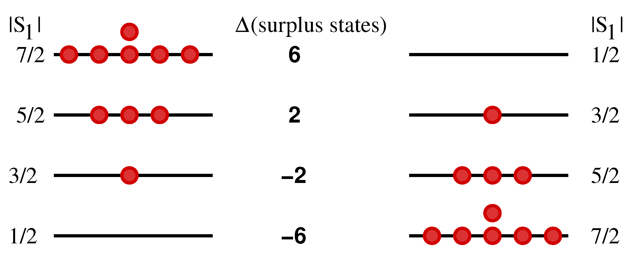
As can be seen in Figure 6, the structure of the trivial (uncoupled) limit superbands depends only on $|S_1|\le S$ and not on spin S itself. We compute the number of quantum states transferred between the energy superbands during the crossover of the trivial limit band structure. This can be done for an arbitrary $S>\frac{1}{2}$, if we first compare all superbands with $|S_1|>\frac{1}{2}$ to the superband $|S_1|=\frac{1}{2}$ with minimal number of states for each $j_1$-value of the integral of motion. This comparison gives the distribution over $j_1$ of the number of surplus states in superband $|S_1|$ (see Figure 8), i.e., states, which do not find counterparts in the superband $|S_1|=\frac{1}{2}$. Manipulation with generating functions [30] allows to obtain an explicit expression for the number of surplus states with given $j_1^{\mathrm{local}}$ for each superband with given $|S_1|$. The same expression can be deduced directly from Figure 9, where the surplus states of the $1:1:2$ spin-oscillator (left column) and missing states of the $1:1:(-2)$ spin-oscillator (right column) are marked by filled and empty red circles, respectively. Thus, the surplus state of the $1:1:2$ Dirac oscillator approximating Hamiltonian (10) with spin-$\frac{3}{2}$ near the pole $(++)$ has an extremal value of $|j_1^{\mathrm{local}}|$.

The number of surplus states in the superband for $|S_1|=\frac{1}{2},\frac{3}{2},\dots ,S-1,S$ is

$$\begin{array}{c}\hfill N_{\mathrm{edge}}^{1:1:2}\left(\right|S_1\left|\right)=\frac{1}{2}\left(|S_1|-\frac{1}{2}\right)\left(|S_1|+\frac{1}{2}\right)\end{array}$$

(20)

In the inverted energy limit, after the crossover, the superband with $|S_1|$ connects to the superband with $|S_1|=S-|S_1|+\frac{1}{2}$ and the number of the surplus states becomes

$$\begin{array}{c}\hfill N_{\mathrm{edge}}^{1:1:2}\left(\right|S-S_1+\frac{1}{2}\left|\right)=\frac{1}{2}(S-|S_1\left|\right)(S-|S_1|+1).\end{array}$$

(21)

The difference in the number of surplus states for the two superbands connected in the crossover gives the number of edge states which are lost/gained by the superband during the rearrangement of the band structure. Even though the corresponding isolated degeneracy point of semi-quantum eigenvalues at $(\mathbf{q},\mathbf{p})=0$ is highly non-generic for large spins $S>\frac{3}{2}$ this works correctly. Figure 8 illustrates rearrangement of surplus states during the crossover of superband structure for $S=7/2$.

According to our general conjecture, which was already used for the $\mathbb{C}$-systems in [1,15], and which we expect to apply to the $\mathbb{H}$-systems as well, the number of gained/lost quantum levels, or the spectral flow, equals the Chern number calculated for the $\Delta$-eigenbundle over the closed surface surrounding the degeneracy point in the full parametric space whose coordinates include slow dynamical variables and formal control parameter. Figure 2, which illustrates the model $\mathbb{C}$-system Hamiltonian (1) of [1], can also represent the full parameter space of the quaternionic Hamiltonian (10) with two slow degrees of freedom or of its local approximations (19). To that end, it is sufficient to imagine that the $\{\mathbf{q},\mathbf{p}\}$ planes in Figure 2 are four dimensional (two degrees of freedom) and the sphere surrounding the isolated degeneracy point at 0 is ${\mathbb{S}}^4$.

For any spin $S>\frac{1}{2}$, the spectral flow equals the difference between the number (20) of surplus states in the trivial limit superband and the number (21) of such states in the reciprocal superband, to which a given superband is connected by the crossover. This spectral flow depends on both S and $|S_1|$, and its general expression reproduces exactly that for the second Chern class

$$\begin{array}{c}\hfill c_2(S,|S_1\left|\right)=v_S\left(\frac{v_S}{2}-\left|S_1\right|\right),\end{array}$$

(22)

with $v_S=(2S+1)/2$ the number of superbands, calculated in [18,19] for the parametric spin-quadrupole system, which we used as the initial point of our dynamical construction. The appearence of the second Chern class (22) as the topological invariant of the model quaternionic systems with Hamiltonians (10) and (19) comes naturally because their semi-quantum energies are double degenerate (form Kramers pairs) everywhere, and the corresponding eigenbundles have rank two.

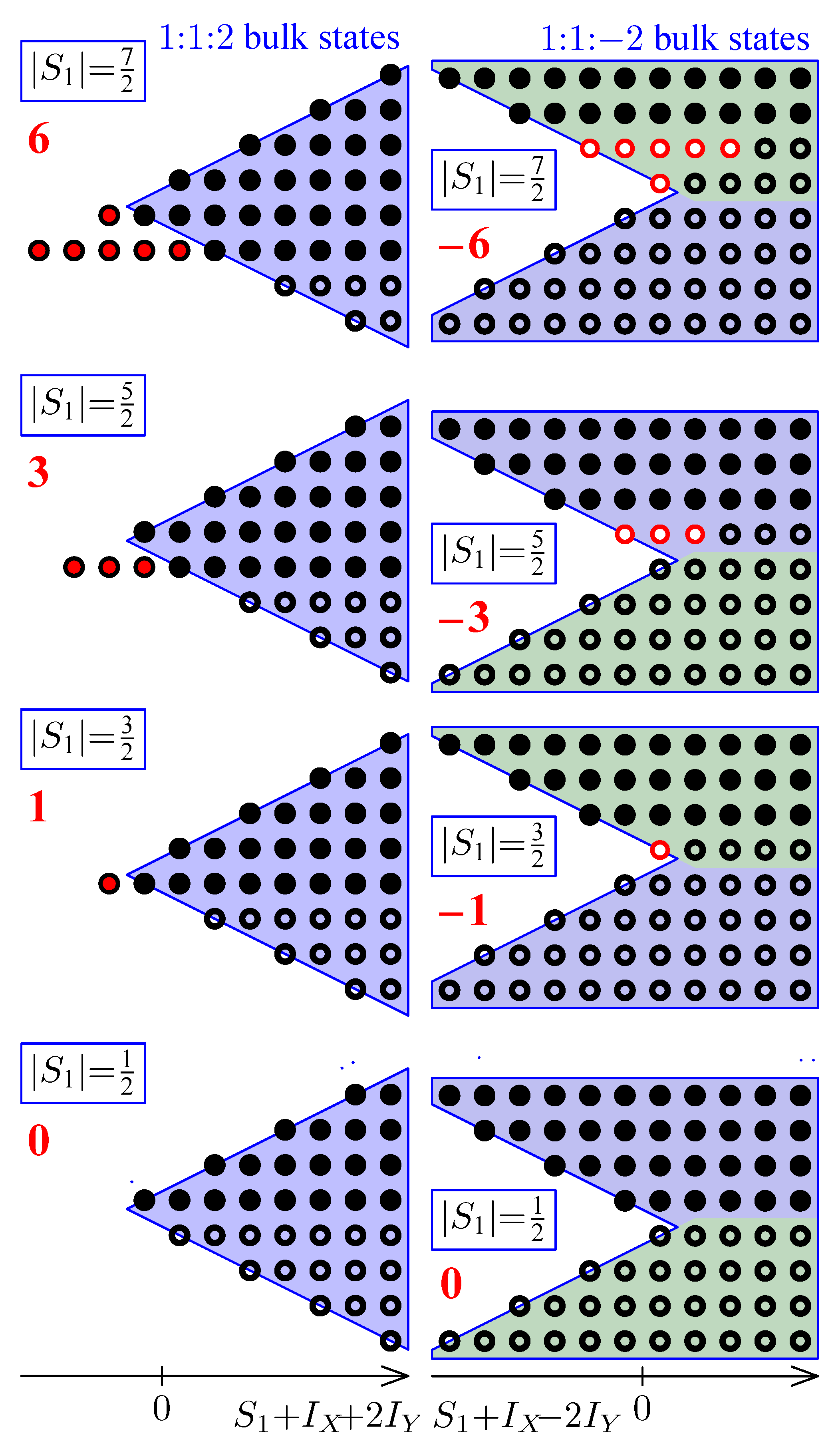
Figure 9 presents another illustration of the above results. It shows the distribution of both edge (surplus) and bulk states for superbands with $S=7/2$. In this figure, the set of uncoupled spin-oscillator basis functions $|S_1,I_X,I_Y\rangle$, with $S_1=-S,-S+1,\dots ,S$, $I_X=0,1,2\dots$, and $I_Y=0,1,2,\dots$ is represented for each superband $|S_1|$ in the form of a lattice in coordinates $\{S_1+I_X\pm 2I_Y,(I_Y+1/2)·\mathrm{sign}(-S_1)\}$. This figure allows to compare resonances $1:1:2$ and $1:1:(-2)$ which correspond to two different types of degeneracies of semi-quantum eigenvalues. As we have seen in Section 2 and Figure 7, both types appear in the example system with Hamiltonian (10) and compact slow classical phase space $P=S^2\times S^2$. To see the similarity between the $1:1:(\pm 2)$ resonances, it is sufficient to replace the concept of “surplus states” by “missing states” or “holes”. This modifies the direction of redistribution while keeping the number of redistributed states (more details will be discussed separately [35]).

Figure 6 represents graphically the way how local figures for spin-oscillators fit within the global representation of the number of state functions for the superbands for quaternionic model with the slow phase space $S^2\times S^2$. Two regions surrounded by red dash lines in the central subfigure of Figure 6 correspond to local lattices represented in Figure 9, left. In these regions, the superbands with $|S_1|>1/2$ have surplus states shown by red dots in Figure 9, left. In a similar way, two fragments surrounded by red dash lines in the bottom part of Figure 6 correspond to lattices for the local $1:1:(-2)$-resonant oscillator models in Figure 9, right. They indicate that the number-of-states distribution of the superbands with $|S_1|=1/2$ and $|S_1|>1/2$ differ in the absence of certain states (or the presence of missing states, which we call “holes”) for $|S_1|>1/2$. The latter are represented by red empty circles in Figure 9, right. The interpretations of the redistribution of quantum states between superbands in terms of surplus states and in terms of holes are complementary. In fact, the replacement of surplus states by holes corresponds to the inversion of the direction of redistribution.

4. Conclusions

Our main result in this paper is the indication of a topological origin of the rearrangement of energy levels between the superbands of quaternionic slow-fast dynamical systems. Such systems comprise a fast subsystem with one degree of freedom (spin) and a slow subsystem with two degrees of freedom, and provide the dynamical realization of the model by Avron et al [17,18] which generalizes the geometric phase setup of Berry [10,11] to the non-Abelian geometric phase. We constructed our example dynamical system with Hamiltonian (10) as a quaternionic generalization of our initial example (1) in [1] which was introduced as a dynamical analog of the original complex parametric Berry Hamiltonian in [10]. The one-parameter family of Hamiltonians (10) describes the generic qualitative phenomenon consisting in redistribution of energy levels between doubly degenerate Kramers superbands. We expose a correspondence between the number of redistributed energy levels and the second Chern class for the eigenbundle of the corresponding semi-quantum Hamiltonian. The most simple elementary qualitative phenomenon for quaternionic Hamiltonians with two slow degrees of freedom, the minimal fast subsystem with two Kramers doublets, and with one additional general control parameter corresponds to the transfer of a single quantum level between two quantum superbands. This transition is associated with the formation of the degeneracy point $(P_{\mathrm{deg}},{\alpha }_{\mathrm{deg}})$ of the eigenvalues of the semi-quantum Hamiltonian. The latter form eigenbundles ${\Delta }_k(P_{\mathrm{deg}},{\alpha }_{\mathrm{deg}})$ with $k=1,2$ over the sphere $S^4$ surrounding the degeneracy point in the total 5-dimensional parameter space of the semi-quantum system. The bundles ${\Delta }_k$ are characterized by the second Chern class $c_2=\pm 1$. Moreover, we demonstrate that the second Chern numbers calculated for the quaternionic model by Avron et al. [18,19] in the case of arbitrarily high half-integer spin S match exactly the number of quantum energy levels transferred between the energy super-bands of the corresponding local dynamical fully quantum model describing the crossover of the Dirac oscillator super-band structure. A more detailed and systematic analysis of the model Hamiltonians, which describe such qualitative modifications of the superband structure, will be given in a separate publication [35] within the framework of constructing dynamical analogs of the complex ($\mathbb{C}$) geometric phase setup by Berry, its generalizations to the quaternionic non-Abelian case ($\mathbb{H}$), and its restriction to the real ($\mathbb{R}$) systems, all inspired by the $\mathbb{R}-\mathbb{C}-\mathbb{H}$ trinity concept in [36].