Cross-Gramian-Based Model Reduction for Descriptor Systems

Abstract

In this paper, we explore model order reduction for large-scale square descriptor systems. A balancing-free square-root method is proposed. The balancing-free square-root method is based on two cross Gramians, one of which is known as the proper cross Gramian and the other as the improper cross Gramian. The proper cross Gramian is the unique solution of a projected generalized continuous-time Sylvester equation, and the improper cross Gramian solves a projected generalized discrete-time Sylvester equation. In order to compute the low-rank factors of these two cross Gramians, we extend the low-rank iteration of the alternating direction implicit method and the Smith method to the projected generalized Sylvester equations. We illustrate the effectiveness of the balance truncation method with one numerical example.

1. Introduction

Model order reduction is essential in many applications. Modern systems are becoming increasingly complex. Usually, at some stage in the design process, it is necessary to use a sufficiently accurate and easy-to-implement reduced order modeling technology. In typical applications, such as the semi-discretization of partial differential equations, VLSI simulation, and multi-body dynamics, the state-space dimension of the system is very large. In all these cases, the direct numerical simulations of such large-scale systems are very expensive so they are not feasible to be implemented in a reasonable computation time. This has inspired the concept of model reduction for large-scale systems (see, for example, [1,2,3,4]).

We consider the model order reduction of a linear continuous-time time-invariant descriptor system formulated using the following differential-algebraic equations:

$$\left\{\begin{array}{ccc}\hfill E\dot{x}\left(t\right)& =& Ax\left(t\right)+Bu\left(t\right),\hfill \\ \hfill y\left(t\right)& =& Cx\left(t\right).\hfill \end{array}\right.$$

(1)

where $x\left(t\right)\in {\mathbb{R}}^n$, $u\left(t\right)\in {\mathbb{R}}^m$, and $y\left(t\right)\in {\mathbb{R}}^p$ are often called the states, the inputs, and the outputs of the system, respectively, and the initial states are $x\left(0\right)=x_0$. The matrices $E\in {\mathbb{R}}^{n\times n},A\in {\mathbb{R}}^{n\times n},B\in {\mathbb{R}}^{n\times m},$ and $C\in {\mathbb{R}}^{p\times n}$ are called the descriptor, state, input, and output matrices. Linear descriptor systems appear frequently in engineering problems including microelectromechanical system design [5] and electrical circuit design [6]. For a comprehensive introduction to the descriptor system, including the structural properties, system realization, and applications, interested readers can refer to the study in [7].

When E is an identity matrix, the system in (1) is called a standard system. There are many model reduction methods for this system. The balanced truncation method [8], which is based on Gramians, is the most classical model reduction method. Other methods based on Gramians include singular perturbation [9] and optimal Hankel norm approximation [10]; see also, for example, [11,12,13] and the references therein. The moment-matching method is another kind of classical model reduction method. It exploits Krylov subspace projections. For a comprehensive review of the moment-matching method, please refer to the study in [14,15]. The balanced truncation method produces stable systems and has bounds on the approximation error between the original systems and reduced systems when it is applied to stable systems. This is its main advantage over the moment-matching method. A main drawback of the balanced truncation method is that we must solve two Lyapunov equations, which makes it impractical for large-scale systems. However, recent developments in efficient implementations of numerical methods for Lyapunov equations make the balanced truncation method attractive for the model reduction of large-scale systems. A balance model reduction has been proposed by applying the balanced truncation method to the cross Gramian [16,17]. This approach is applied to symmetric systems and only needs to solve one Sylvester equation. To make the cross-Gramian approach suitable for nonsymmetric systems, a symmetrizer must be established (see, e.g., [17]).

For the model order reduction of the descriptor system in (1), we want to establish a reduced-order descriptor, which has fewer states and is of the same form as (1). The reduced-order system has the following form:

$$\left\{\begin{array}{ccc}\hfill \widehat{E}\dot{\widehat{x}}\left(t\right)& =& \widehat{A}\widehat{x}\left(t\right)+\widehat{B}u\left(t\right),\hfill \\ \hfill y\left(t\right)& =& \widehat{C}\widehat{x}\left(t\right),\hfill \end{array}\right.$$

(2)

where the matrices $\widehat{E},\widehat{A}\in {\mathbb{R}}^{l\times l}$, $\widehat{B}\in {\mathbb{R}}^{l\times m}$, and $\widehat{C}\in {\mathbb{R}}^{p\times l}$ have fewer orders.

The balanced truncation model reduction method was extended to descriptor systems by Stykel [18]. This approach is based on four Gramians (two controllability Gramians and two observability Gramians). The main computational work is to solve two projected generalized continuous-time Lyapunov equations (PGCTLEs) and two projected generalized discrete-time Lyapunov equations (PGDTLEs). The low-rank factors of the controllability Gramian and observability Gramian can be efficiently computed by applying the low-rank ADI iteration (LR-ADI) and the low-rank Smith iteration to the projected Lyapunov equations (see, for example, [19]).

Inspired by the ideas in [16,17] for standard square systems, we propose in this paper a model reduction method based on cross Gramians for large-scale square descriptor systems. This method is equivalent to the Gramian-based model reduction method presented in [18] under some conditions. In this approach, we only need to solve two projected generalized Sylvester equations. These two solutions are the proper cross Gramian and the improper cross Gramian of the square descriptor system, respectively. For computing the low-rank factors of the proper cross Gramian and the improper cross Gramian, we extend the LR-ADI and the LR-Smith to the projected Sylvester equations.

So, the main contribution of this paper is the proposal of a cross-Gramian-based balanced truncation model reduction for descriptor systems. For a SISO or a special square descriptor system, we show that the cross-Gramian-based method and the Gramian-based method theoretically generate the same reduced system. For square nonsymmetric systems, it is shown through numerical experiments that the cross-Gramian-based method generates more accurate reduced systems in the low-frequency range than the Gramian-based method.

In this paper, we use the following notations. ${\mathbb{R}}^{m\times n}$ denotes the linear space of the real $m\times n$ matrices. The spectral radius of $A\in {\mathbb{R}}^{n\times n}$ is denoted by $\rho \left(A\right)$. The 2-norm and the Frobenius norms of a matrix are ${\parallel A\parallel }_2$ and ${\parallel A\parallel }_F$ and $\kappa \left(A\right)={\parallel A\parallel }_2{\parallel A^{-1}\parallel }_2$ is called the condition number of the invertible matrix A.

The structure of the paper is as follows. We first review some concepts and results of descriptor systems in Section 2 and then we outline the balanced truncation for descriptor systems. The LR-ADI iteration and the Smith iteration for solving the projected Lyapunov equations are listed for comparison. In Section 3, we propose a balancing-free square-root model order reduction method for square descriptor systems. Numerical methods for solving projected Sylvester equations are also developed. The numerical experiments are presented in Section 4. Finally, we provide conclusions in Section 5.

2. Model Reduction Based on Gramians

We first introduce some basic notations and briefly review the concepts of controllability, observability, Hankel singular values, and balanced realization, and several important results of studies on descriptor systems. Then we outline a balancing-free square-root (BFSR) method for the model reduction of descriptor systems. Varga [20] first proposed the BFSR method for standard systems. Stykel [18] generalized this method to descriptor systems. Much of the material in this section is standard and can be found in [18,21].

2.1. Preliminaries

It is known that $E,A$ have Weierstrass canonical decompositions [22]:

$$E=W\left[\begin{array}{cc}I& 0\\ 0& N\end{array}\right]T,A=W\left[\begin{array}{cc}J& 0\\ 0& I\end{array}\right]T,$$

(3)

where $W,T$ are nonsingular and $J\in {\mathbb{R}}^{n_f\times n_f},$ $N\in {\mathbb{R}}^{n_{\infty }\times n_{\infty }}$ are the block diagonal matrices. We point out that each diagonal block is a Jordan block. The diagonal elements of J are the finite eigenvalues of the pencil $\lambda E-A$. The nilpotency index $\nu$ of N is named as the index of the pencil $\lambda E-A$.

Based on (3), we define $P_l$, $P_r$ as

$$P_l=W\left[\begin{array}{cc}I& 0\\ 0& 0\end{array}\right]W^{-1},P_r=T^{-1}\left[\begin{array}{cc}I& 0\\ 0& 0\end{array}\right]T.$$

(4)

We know that $P_r$ and $P_l$ are the right and left deflating subspaces, which correspond to the finite eigenvalues of the pencil $\lambda E-A$, respectively.

Assume that the input $u\left(t\right)=0$ for $t<0$ and the initial state $x\left(0\right)=0$. Then, by taking the Laplace transform of the descriptor system in (1), we have

$$\left\{\begin{array}{ccc}\hfill sEx\left(s\right)& =& Ax\left(s\right)+Bu\left(s\right),\hfill \\ \hfill y\left(s\right)& =& Cx\left(s\right),\hfill \end{array}\right.$$

(5)

where $x\left(s\right),y\left(s\right),u\left(s\right)$ represent the Laplace transforms of $x\left(t\right),y\left(t\right),u\left(t\right)$, respectively. Eliminating $x\left(s\right)$ in (5) results in the frequency domain of the input–output relation $y\left(s\right)=H\left(s\right)u\left(s\right)$, where $H\left(s\right)$ is the transfer function

$$H\left(s\right)=C{(sE-A)}^{-1}B.$$

For simplicity, we also denote the descriptor system in (1) by $(E,A,B,C)$. Two systems $(E,A,B,C)$ and $(\tilde{E},\tilde{A},\tilde{B},\tilde{C})$ are called the restricted system equivalents if there exist nonsingular matrices $\tilde{W},\tilde{T}\in {\mathbb{R}}^{n\times n}$ such that

$$\tilde{E}=\tilde{W}E\tilde{T},\tilde{A}=\tilde{W}A\tilde{T},\tilde{B}=\tilde{W}B,C=C\tilde{T}.$$

The pair $(\tilde{W},\tilde{T})$ is called the system equivalence transformation. Note that under any system equivalence transformation, the transfer function of the descriptor system in (1) is invariant, i.e.,

$$H\left(s\right)=C{(sE-A)}^{-1}B=\tilde{C}{(s\tilde{E}-\tilde{A})}^{-1}\tilde{B}=\tilde{H}\left(s\right).$$

We assume that the descriptor system in (1) is stable, that is, the real parts of all finite eigenvalues of $\lambda E-A$ are negative. As is shown in [18,21], the transfer function $H\left(s\right)$ can be written as

$$H\left(s\right)=H_{sp}\left(s\right)+P\left(s\right),$$

where

$$H_{sp}\left(s\right)=C{P}_r{(sE-A)}^{-1}{P}_{l}B,P\left(s\right)=C(I-P_r){(sE-A)}^{-1}(I-P_l)B$$

are the strictly proper part and the polynomial part of $H\left(s\right)$, respectively. For the strictly proper part $H_{sp}$, its ${\mathbb{H}}_{\infty }$ norm is defined by

$$\parallel H_{sp}{\parallel }_{{\mathbb{H}}_{\infty }}=\underset{\omega \in \mathbb{R}}{sup}{\parallel H_{sp}\left(i\omega \right)\parallel }_2.$$

Definition 1

([7,21,23,24]). The descriptor system $H\left(s\right)=C{(sE-A)}^{-1}B$ is called completely controllable if

$$\mathrm{rank}\left(\right[\alpha E-\beta A,B\left]\right)=n,\forall (\alpha ,\beta )\in (\mathbb{C}\times \mathbb{C})\backslash \left\{\right(0,0\left)\right\},$$

and completely observable if square root

$$\mathrm{rank}\left([\alpha E^T-\beta A^T,C^T]\right)=n,\forall (\alpha ,\beta )\in (\mathbb{C}\times \mathbb{C})\backslash \left\{(0,0)\right\}.$$

Partition $W^{-1}B$ and $C{T}^{-1}$ in blocks conformably to E and A in (3) as

$$W^{-1}B=\left[\begin{array}{c}{B}_1\\ B_2\end{array}\right],C{T}^{-1}=\left[\begin{array}{cc}{C}_1& C_2\end{array}\right].$$

Then, the following results hold for the descriptor system in (1) to be completely controllable and completely observable.

Theorem 1

([7,21,23,24]). Assume that $\lambda E-A$ is a regular pencil. Then, the following statements are equivalent:

(a) 

the descriptor system $H\left(s\right)=C{(sE-A)}^{-1}B$ is completely controllable;

(b) 

$\mathrm{rank}\left(\right[\lambda E-A,B\left]\right)=n$ for all $\lambda \in \mathbb{C}$ and $\mathrm{rank}\left(\right[E,B\left]\right)=n$;

(c) 

$\mathrm{rank}\left([\lambda I-J,B_1]\right)=n_f$ for all $\lambda \in \mathbb{C}$ and $\mathrm{rank}\left([N,B_2]\right)=n_{\infty }$;

(d) 

$\mathrm{rank}\left([B_1,J{B}_1,\dots ,J^{n_f-1}{B}_1]\right)=n_f$ and $\mathrm{rank}\left([B_2,N{B}_2,\dots ,N^{\nu -1}{B}_2]\right)=n_{\infty }$.

Theorem 2

([7,21,23,24]). Assume that $\lambda E-A$ is a regular pencil. Then, the following statements are equivalent:

(a) 

the descriptor system $H\left(s\right)=C{(sE-A)}^{-1}B$ is completely observable;

(b) 

$\mathrm{rank}\left([\lambda E^T-A^T,C^T]\right)=n$ for all $\lambda \in \mathbb{C}$ and $\mathrm{rank}\left([E^T,C^T]\right)=n$;

(c) 

$\mathrm{rank}\left([\lambda I-J^T,C_1^T]\right)=n_f$ for all $\lambda \in \mathbb{C}$ and $\mathrm{rank}\left([N^T,C_2^T]\right)=n_{\infty }$;

(d) 

$\mathrm{rank}\left([C_1^T,J^T{C}_1^T,\dots ,{\left(J^{n_f-1}\right)}^T{C}_1^T]\right)=n_f$ and $\mathrm{rank}\left([C_2^T,N^T{C}_2^T,\dots ,{\left(N^{\nu -1}\right)}^T{C}_2^T]\right)=n_{\infty }$.

Define

$${\mathcal{G}}_{pc}={\int }_0^{\infty }\mathcal{F}\left(t\right)B{B}^T{\mathcal{F}}^T\left(t\right)dt,{\mathcal{G}}_{po}={\int }_0^{\infty }{\mathcal{F}}^T\left(t\right)C^{T}C\mathcal{F}\left(t\right)dt,$$

where

$$\mathcal{F}\left(t\right)=T^{-1}\left[\begin{array}{cc}{e}^{Jt}& 0\\ 0& 0\end{array}\right]W^{-1}.$$

The matrices ${\mathcal{G}}_{pc},{\mathcal{G}}_{po}$ are the proper controllability and observability Gramians. We also define

$${\mathcal{G}}_{ic}=\sum _{k=0}^{\nu -1}{F}_{k}B{B}^T{F}_k^T,{\mathcal{G}}_{io}=\sum _{k=0}^{\nu -1}{F}_k^T{C}^{T}C{F}_k,$$

where

$$F_k=T^{-1}\left[\begin{array}{cc}0& 0\\ 0& -N^k\end{array}\right]W^{-1},k=0,1,\dots ,\nu -1.$$

The matrices ${\mathcal{G}}_{ic},{\mathcal{G}}_{io}$ are the improper controllability and observability Gramians, respectively.

Concerning the proper and improper Gramians, we have the following results.

Theorem 3

([18,21]). Let the pencil $\lambda E-A$ be stable. Then, the PGCTLEs

$$\begin{array}{ccc}& & A{\mathcal{G}}_{pc}{E}^T+E{\mathcal{G}}_{pc}{A}^T+P_{l}B{B}^T{P}_l^T=0,{\mathcal{G}}_{pc}=P_r{\mathcal{G}}_{pc}{P}_r^T,\hfill \end{array}$$

(6)

$$\begin{array}{ccc}& & A^T{\mathcal{G}}_{po}E+E^T{\mathcal{G}}_{po}A+P_r^T{C}^{T}C{P}_r=0,{\mathcal{G}}_{po}=P_l^T{\mathcal{G}}_{po}{P}_l,\hfill \end{array}$$

(7)

have unique symmetric, positive semidefinite solutions. Similarly, the unique solutions of the PGDTLEs

$$\begin{array}{ccc}& & A{\mathcal{G}}_{ic}{A}^T-E{\mathcal{G}}_{ic}{E}^T=(I-P_l)B{B}^T{(I-P_l)}^T,P_r{\mathcal{G}}_{ic}{P}_r^T=0,\hfill \end{array}$$

(8)

$$\begin{array}{ccc}& & A^T{\mathcal{G}}_{io}A-E^T{\mathcal{G}}_{io}E={(I-P_r)}^T{C}^{T}C(I-P_r),P_l^T{\mathcal{G}}_{io}{P}_l=0.\hfill \end{array}$$

(9)

are also symmetric, positive semidefinite. Moreover, the eigenvalues of ${\mathcal{G}}_{pc}{E}^T{\mathcal{G}}_{po}E$ and ${\mathcal{G}}_{ic}{A}^T{\mathcal{G}}_{io}A$ are non-negative.

Definition 2

([18,21]). Suppose that $\lambda E-A$ is a stable pencil. Let $n_f$, $n_{\infty }$ be the dimensions of the deflating subspaces of its finite and infinite eigenvalues, respectively. Then,

• the proper Hankel singular values ${\zeta }_i$ are defined as the square roots of the largest $n_f$ eigenvalues of ${\mathcal{G}}_{pc}{E}^T{\mathcal{G}}_{po}E$.
• the improper Hankel singular values ${\theta }_i$ are defined as the square roots of the largest $n_{\infty }$ eigenvalues of ${\mathcal{G}}_{ic}{A}^T{\mathcal{G}}_{io}A$.

It was shown in [18,21] that after applying an equivalence transformation $(\tilde{W},\tilde{T})$ to the system, two controllability Gramians ${\mathcal{G}}_{pc}$ and ${\mathcal{G}}_{ic}$ turn into

$${\tilde{\mathcal{G}}}_{pc}={\tilde{T}}^{-1}{\mathcal{G}}_{pc}{\tilde{T}}^{-T},{\tilde{\mathcal{G}}}_{ic}={\tilde{T}}^{-1}{\mathcal{G}}_{ic}{\tilde{T}}^{-T}.$$

Similarly, two observability Gramians ${\mathcal{G}}_{po}$ and ${\mathcal{G}}_{io}$ become

$${\tilde{\mathcal{G}}}_{po}={\tilde{W}}^{-T}{\mathcal{G}}_{po}{\tilde{W}}^{-1},{\tilde{\mathcal{G}}}_{io}={\tilde{W}}^{-T}{\mathcal{G}}_{io}{\tilde{W}}^{-1}.$$

Moreover,

$${\tilde{\mathcal{G}}}_{pc}{\tilde{E}}^T{\tilde{\mathcal{G}}}_{po}\tilde{E}={\tilde{T}}^{-1}{\mathcal{G}}_{pc}{E}^T{\mathcal{G}}_{po}E\tilde{T},{\tilde{\mathcal{G}}}_{ic}{\tilde{A}}^T{\tilde{\mathcal{G}}}_{io}\tilde{A}={\tilde{T}}^{-1}{\mathcal{G}}_{ic}{E}^T{\mathcal{G}}_{io}E\tilde{T}.$$

Thus, under any system equivalence transformation, the proper and improper Hankel singular values of the descriptor system in (1) are invariant.

The concepts of the balanced realization and balance transformation of the standard state-space system are generalized to the descriptor system in (1) as follows.

Definition 3

([18,21]). Define $\mathrm{\Sigma }=\mathrm{diag}({\zeta }_1,{\zeta }_2,\dots ,{\zeta }_{n_f})$ and $\mathrm{\Theta }=\mathrm{diag}({\theta }_1,{\theta }_2,\dots ,{\theta }_{n_{\infty }})$. If

$${\mathcal{G}}_{po}={\mathcal{G}}_{pc}=\left[\begin{array}{cc}\mathrm{\Sigma }& 0\\ 0& 0\end{array}\right],{\mathcal{G}}_{io}={\mathcal{G}}_{ic}=\left[\begin{array}{cc}0& 0\\ 0& \mathrm{\Theta }\end{array}\right],$$

then $(E,A,B,C)$ is called a balanced system.

Definition 4

([18,21]). The system equivalence transformation $(W_b,T_b)$ of the descriptor system in (1) is called a balance transformation if the transformed realization $(W_{b}E{T}_b,W_{b}A{T}_b,W_{b}B,C{T}_b)$ is balanced.

2.2. Model Reduction Based on Gramians for Descriptor Systems

It is well known that Gramians are essential in a balanced truncation for standard state-space systems. In this subsection, we outline the generalization for descriptor systems.

Define the Cholesky factorizations [25] for the proper and improper Gramians as follows:

$${\mathcal{G}}_{pc}=R_p{R}_p^T,{\mathcal{G}}_{po}=L_p{L}_p^T,{\mathcal{G}}_{ic}=R_i{R}_i^T,{\mathcal{G}}_{io}=L_i{L}_i^T.$$

where $R_p,L_p,R_i,L_i\in {\mathbb{R}}^{n\times n}$ are the lower triangular matrices.

Then, we define the singular value decompositions [25] of $L_p^{T}E{R}_p$ and $L_i^{T}A{R}_i$ as follows:

$$L_p^{T}E{R}_p=U_p\mathrm{\Sigma }{V}_p^T,L_i^{T}A{R}_i=U_i\mathrm{\Theta }{V}_i^T.$$

Here, $U_p,V_p,U_i,V_i$ are orthogonal, and $\mathrm{\Sigma }=\mathrm{diag}({\zeta }_1,{\zeta }_2,\dots ,{\zeta }_{n_f})$, $\mathrm{\Theta }=\mathrm{diag}({\theta }_1,{\theta }_2,\dots ,{\theta }_{n_{\infty }})$. It was shown in [18,21] that if the descriptor system in (1) is completely controllable and completely observable, then the system equivalence transformation $(W_b,T_b)$ defined by

$$W_b=\left[\begin{array}{c}{\mathrm{\Sigma }}^{-1/2}{U}_p^T{L}_p^T\\ {\mathrm{\Theta }}^{-1/2}{U}_i^T{L}_i^T\end{array}\right],T_b=[R_p{V}_p{\mathrm{\Sigma }}^{-1/2},R_i{V}_i{\mathrm{\Theta }}^{-1/2}],$$

is a balance transformation of (1).

In [18], a balanced truncation square-root method was proposed for the model reduction of the descriptor system in (1). It is a direct generalization of the balanced truncation square-root method for standard state-space systems.

As pointed out in [18], when the system is highly unbalanced, the balanced truncation square-root method may be unstable. This will also happen when the deflating subspaces of the finite and infinite eigenvalues have a small angle. To overcome this disadvantage, Stykel proposed a BFSR model reduction method for descriptor systems, which is a generalization of the BFSR method proposed in [20] for standard linear systems. This BFSR model reduction method for the descriptor system in (1) is described in Algorithm 1.

Algorithm 1The BFSR method based on Gramians

Input:  the system matrices $E,A,B,C$. Output:  the reduced system matrices $\widehat{E},\widehat{A},\widehat{B},\widehat{C}$.   Compute the low-rank factors $R_p,L_p,R_i,L_i$ of ${\mathcal{G}}_{pc},{\mathcal{G}}_{po}$, ${\mathcal{G}}_{ic},{\mathcal{G}}_{io}$.   Compute the skinny SVD $$L_p^{T}E{R}_p=\left[\begin{array}{cc}{U}_1& U_2\end{array}\right]\left[\begin{array}{cc}{\mathrm{\Sigma }}_1& 0\\ 0& {\mathrm{\Sigma }}_2\end{array}\right]{\left[\begin{array}{cc}{V}_1& V_2\end{array}\right]}^T$$   with ${\mathrm{\Sigma }}_1=\mathrm{diag}({\zeta }_1,{\zeta }_2,\dots ,{\zeta }_{l_f})$ and ${\mathrm{\Sigma }}_2=\mathrm{diag}({\zeta }_{l_f+1},{\zeta }_{l_f+2},\dots ,{\zeta }_{r_p})$ with $r_p=\mathrm{rank}\left(L_p^{T}E{R}_p\right)$.   Compute the skinny SVD $$L_i^{T}A{R}_i=U_3\mathrm{\Theta }{V}_3^T,$$   where $\mathrm{\Theta }=\mathrm{diag}({\theta }_1,{\theta }_2,\dots ,{\theta }_{l_{\infty }})$ and $l_{\infty }=\mathrm{rank}\left(L_i^{T}A{R}_i\right)$.   Compute the skinny QR factorization $$[R_p{V}_1,R_i{V}_3]=Q_R{R}_0,[L_p{U}_1,L_i{U}_3]=Q_L{L}_0,$$   where the columns of $Q_R,Q_L$ are orthonormal and those of $R_0,L_0$ are nonsingular.   Construct a reduced system $$(\widehat{E},\widehat{A},\widehat{B},\widehat{C})=(Q_L^{T}E{Q}_R,Q_L^{T}A{Q}_R,Q_L^{T}B,C{Q}_R).$$

As shown in [18,26], the reduced system $\widehat{H}\left(s\right)$ generated by the BFSR method is also stable if the original system in (1) is c-stable. Moreover, the upper bound on the ${\mathbb{H}}_{\infty }$ norm of the error between the original system and the reduced system is given by

$$\parallel H-\widehat{H}{\parallel }_{{\mathbb{H}}_{\infty }}\le 2({\zeta }_{l_f+1}+{\zeta }_{l_f+2}+\dots +{\zeta }_{n_f}).$$

(10)

The main computational work in the BFSR method based on Gramians is to compute the low-rank factors of the solutions of the PGCTLEs ((6) and (7)) and the PGDTLEs ((8) and (9)). The low-rank factors of Gramians can be computed efficiently by the LR-ADI and the LR-Smith [19]. These two methods are generalizations of the well-known LR-ADI and LR-Smith [27] for standard continuous-time and discrete-time Lyapunov equations. For completeness and comparison, we outline the LR-ADI and LR-Smith for solving the PGCTLEs and PGDTLEs in Algorithms 2 and 3, respectively. In [19,28], it was also proposed how we should choose the shift parameters in the LR-ADI iteration.

Algorithm 2LR-ADI for PGCTLE

Input:  $E,A,B$; the shifts $\{{\tau }_1,{\tau }_2,\dots ,{\tau }_s\}$. Output:  $Z_k$ such that $Z_k{Z}_k^T$ is an approximate solution of the PGCTLE (6).   Compute $Z^{\left(1\right)}=\sqrt{-2\mathrm{Re}\left({\tau }_1\right)}{(E+{\tau }_{1}A)}^{-1}{P}_{l}B$;   Set $Z_1=Z^{\left(1\right)}$;   For $k=2,3,\dots$       $Z^{\left(k\right)}=\sqrt{\frac{\mathrm{Re}\left({\tau }_k\right)}{\mathrm{Re}\left({\tau }_{k-1}\right)}}[I-({\overline{\tau }}_{k-1}+{\tau }_k){(E+{\tau }_{k}A)}^{-1}A]Z^{(k-1)}$;       $Z_k=[Z_{k-1},Z^{\left(k\right)}]$;   End For

Algorithm 3LR-Smith for PGDTLE

Input:  $E,A,B$. Output:  ${\tilde{Z}}_k$ such that ${\tilde{Z}}_k{\tilde{Z}}_k^T$ is a solution of the PGDTLE (8).   ${\tilde{Z}}^{\left(1\right)}=A^{-1}(I-P_l)B$;   Set ${\tilde{Z}}_1={\tilde{Z}}^{\left(1\right)}$;   For $k=2,3,\dots ,\nu$        ${\tilde{Z}}^{\left(k\right)}=A^{-1}E{\tilde{Z}}^{(k-1)}$;        ${\tilde{Z}}_k=[{\tilde{Z}}_{k-1},{\tilde{Z}}^{\left(k\right)}]$;   End For

3. Model Reduction Based on Cross Gramians

In this section, we consider the model reduction method based on cross Gramians for square descriptor systems. First, we present the definition of the proper cross Gramian and improper cross Gramian and show that the proper cross Gramian of the square descriptor system in (1) is the unique solution of a projected generalized continuous-time Sylvester equation (PGCTSE), whereas the improper cross Gramian is the unique solution of a projected generalized discrete-time Sylvester equation (PGDTSE). Then, a balancing transformation for the square descriptor system in (1) is established by exploiting the proper cross Gramian and improper cross Gramian. Finally, we develop a cross-Gramian-based BFSR model reduction method. Moreover, we also consider the numerical solution of the PGCTSE and PGDTSE and generalize the LR-ADI and LR-Smith methods to these two matrix equations.

3.1. Cross-Gramian-Based Balanced Realization

Cross Gramians [17,29] are another kind of Gramian and are defined only for standard square systems. We can extend them to a square descriptor system as follows.

Definition 5.

For a stable square descriptor system $H\left(s\right)=C{(sE-A)}^{-1}B$, its proper cross Gramian is defined as

$$X={\int }_0^{\infty }\mathcal{F}\left(t\right)BC\mathcal{F}\left(t\right)dt$$

(11)

and its improper cross Gramian is defined as

$$Y=\sum _{k=0}^{\nu -1}{F}_{k}BC{F}_k.$$

(12)

It is easy to show that the proper cross Gramian X is the unique solution of the PGCTSE

$$AXE+EXA+P_{l}BC{P}_r=0,X=P_{r}X{P}_l,$$

(13)

whereas the improper cross Gramian Y is the unique solution of the PGDTSE

$$AYA-EYE=(I-P_l)BC(I-P_r),P_{r}Y{P}_l=0.$$

(14)

Theorem 4.

Let (1) be a SISO descriptor system or a square descriptor system with $C{\left(PA\right)}^{k}PB={(C{\left(PA\right)}^{k}PB)}^T$ for all $k\ge 0$, where

$$P=T^{-1}\left[\begin{array}{cc}I& 0\\ 0& 0\end{array}\right]W^{-1}.$$

Assume that this system is completely controllable and completely observable. Then, we have

$${\left(XE\right)}^2={\mathcal{G}}_{pc}{E}^T{\mathcal{G}}_{po}E.$$

Proof. 

Define

$$\widehat{X}=TXW=\left[\begin{array}{cc}{\widehat{X}}_{11}& {\widehat{X}}_{12}\\ {\widehat{X}}_{21}& {\widehat{X}}_{22}\end{array}\right],$$

where ${\widehat{X}}_{11}\in {\mathbb{R}}^{n_f\times n_f}$, ${\widehat{X}}_{22}\in {\mathbb{R}}^{n_{\infty }\times n_{\infty }}$, ${\widehat{X}}_{12}\in {\mathbb{R}}^{n_f\times n_{\infty }}$, and ${\widehat{X}}_{21}\in {\mathbb{R}}^{n_{\infty }\times n_f}$.

Partition $W^{-1}B$ and $C{T}^{-1}$ appropriately as

$$W^{-1}B=\left[\begin{array}{c}{B}_1\\ B_2\end{array}\right],C{T}^{-1}=\left[\begin{array}{cc}{C}_1& C_2\end{array}\right].$$

We can show that the solution X of the PGCTSE (13) can be formulated as

$$X=T^{-1}\left(\begin{array}{cc}{\widehat{X}}_{11}& 0\\ 0& 0\end{array}\right)W^{-1},$$

(15)

where ${\widehat{X}}_{11}$ is the solution of

$$J{\widehat{X}}_{11}+{\widehat{X}}_{11}J+B_1{C}_1=0.$$

(16)

Correspondingly, the solutions ${\mathcal{G}}_{pc}$ and ${\mathcal{G}}_{po}$ of the PGCTLEs ((6) and (8)) can be expressed as

$$\begin{array}{ccc}\hfill {\mathcal{G}}_{pc}& =& T^{-1}\left(\begin{array}{cc}{\widehat{\mathcal{G}}}_{pc}^{\left(11\right)}& 0\\ 0& 0\end{array}\right)T^{-T},\hfill \end{array}$$

(17)

$$\begin{array}{ccc}\hfill {\mathcal{G}}_{po}& =& W^{-T}\left(\begin{array}{cc}{\widehat{\mathcal{G}}}_{po}^{\left(11\right)}& 0\\ 0& 0\end{array}\right)W^{-1},\hfill \end{array}$$

(18)

where ${\widehat{\mathcal{G}}}_{pc}^{\left(11\right)}$ and ${\mathcal{G}}_{po}^{\left(11\right)}$ are, respectively, the solutions of

$$\begin{array}{cc}& J{\widehat{\mathcal{G}}}_{pc}^{\left(11\right)}+{\widehat{\mathcal{G}}}_{pc}^{\left(11\right)}{J}^T+B_1{B}_1^T=0,\end{array}$$

(19)

$$\begin{array}{cc}& J^T{\widehat{\mathcal{G}}}_{po}^{\left(11\right)}+{\widehat{\mathcal{G}}}_{po}^{\left(11\right)}J+C_1^T{C}_1=0.\end{array}$$

(20)

Since $H\left(s\right)=C{(sE-A)}^{-1}B$ is completely controllable and completely observable, it follows from Theorems 1 and 2 that the standard stable system $C_1{(sI-J)}^{-1}{B}_1$ is controllable and observable. On the one hand, if $H\left(s\right)$ is a SISO system, then $C_1{(sI-J)}^{-1}{B}_1$ is also a SISO system. On the other hand, if $H\left(s\right)$ is a system with $C{\left(PA\right)}^{k}PB={(C{\left(PA\right)}^{k}PB)}^T$ for all $k\ge 0$, it is easy to verify that $C_1{J}^k{B}_1={\left(C_1{J}^k{B}_1\right)}^T$ for all $k\ge 0$, i.e., $C_1{(sI-J)}^{-1}{B}_1$ is a symmetric system. Thus, from [17], it follows that ${\widehat{X}}_{11}^2={\widehat{\mathcal{G}}}_{pc}^{\left(11\right)}{\widehat{\mathcal{G}}}_{po}^{\left(11\right)}$, and ${\widehat{X}}_{11}$ can be decomposed into ${\widehat{X}}_{11}=Z_X{D}_X{Z}_X^{-1}$ with $D_X$ being a real diagonal nonsingular matrix.

It follows from (15) and (3) that

$$XE=T^{-1}\left(\begin{array}{cc}{\widehat{X}}_{11}& 0\\ 0& 0\end{array}\right)W^{-1}W\left[\begin{array}{cc}I& 0\\ 0& N\end{array}\right]T=T^{-1}\left(\begin{array}{cc}{\widehat{X}}_{11}& 0\\ 0& 0\end{array}\right)T.$$

Thus, we obtain

$${\left(XE\right)}^2=T^{-1}\left(\begin{array}{cc}{\widehat{X}}_{11}^2& 0\\ 0& 0\end{array}\right)T.$$

By (17), (18), and (3), we obtain

$${\mathcal{G}}_{pc}{E}^T{\mathcal{G}}_{po}E=T^{-1}\left(\begin{array}{cc}{\widehat{\mathcal{G}}}_{pc}^{\left(11\right)}{\widehat{\mathcal{G}}}_{po}^{\left(11\right)}& 0\\ 0& 0\end{array}\right)T.$$

(21)

Thus,

$${\left(XE\right)}^2={\mathcal{G}}_{pc}{E}^T{\mathcal{G}}_{po}E.$$

   □

Theorem 5.

Let (1) be a SISO descriptor system or a square descriptor system with $C{(\tilde{P}A)}^k\tilde{P}B={(C{(\tilde{P}A)}^k\tilde{P}B)}^T$ for all $k\ge 0$, where

$$\tilde{P}=T^{-1}\left[\begin{array}{cc}0& 0\\ 0& I\end{array}\right]W^{-1}.$$

Assume that $H\left(s\right)=C{(sE-A)}^{-1}B$ is completely controllable and completely observable. Then, we have

$${\left(YA\right)}^2={\mathcal{G}}_{ic}{A}^T{\mathcal{G}}_{io}A.$$

Proof. 

Define

$$\widehat{Y}=TYW=\left[\begin{array}{cc}{\widehat{Y}}_{11}& {\widehat{Y}}_{12}\\ {\widehat{Y}}_{21}& {\widehat{Y}}_{22}\end{array}\right],$$

where ${\widehat{Y}}_{11}\in {\mathbb{R}}^{n_f\times n_f}$, ${\widehat{Y}}_{22}\in {\mathbb{R}}^{n_{\infty }\times n_{\infty }}$, ${\widehat{Y}}_{12}\in {\mathbb{R}}^{n_f\times n_{\infty }}$, and ${\widehat{Y}}_{21}\in {\mathbb{R}}^{n_{\infty }\times n_f}$.

Similarly, it is easy to show that the solution Y of the PGDTSE (14) can be formulated as

$$Y=T^{-1}\left(\begin{array}{cc}0& 0\\ 0& {\widehat{Y}}_{22}\end{array}\right)W^{-1},$$

(22)

where ${\widehat{Y}}_{22}$ is the solution of

$${\widehat{Y}}_{22}-N{\widehat{Y}}_{22}N=B_2{C}_2.$$

That is, ${\widehat{Y}}_{22}$ can be formulated as

$${\widehat{Y}}_{22}=\sum _{k=0}^{\gamma -1}{N}^k{B}_2{C}_2{N}^k.$$

We now consider the improper Gramians ${\mathcal{G}}_{ic}$ and ${\mathcal{G}}_{io}$, which are, respectively, the solutions of these two PGDTLEs ((7) and (9)). We have

$$\begin{array}{ccc}\hfill {\mathcal{G}}_{ic}& =& T^{-1}\left(\begin{array}{cc}0& 0\\ 0& {\widehat{\mathcal{G}}}_{ic}^{\left(22\right)}\end{array}\right)T^{-T},\hfill \end{array}$$

(23)

$$\begin{array}{ccc}\hfill {\mathcal{G}}_{io}& =& W^{-T}\left(\begin{array}{cc}0& 0\\ 0& {\widehat{\mathcal{G}}}_{io}^{\left(22\right)}\end{array}\right)W^{-1},\hfill \end{array}$$

(24)

where ${\widehat{\mathcal{G}}}_{ic}^{\left(22\right)}$ and ${\mathcal{G}}_{io}^{\left(22\right)}$ are the solutions of

$$\begin{array}{cc}& {\widehat{\mathcal{G}}}_{ic}^{\left(22\right)}-N{\widehat{\mathcal{G}}}_{ic}^{\left(22\right)}{N}^T=B_2{B}_2^T,\hfill \\ & {\widehat{\mathcal{G}}}_{io}^{\left(22\right)}-N^T{\widehat{\mathcal{G}}}_{io}^{\left(22\right)}N=C_2^T{C}_2,\hfill \end{array}$$

i.e.,

$${\widehat{\mathcal{G}}}_{ic}^{\left(22\right)}=\sum _{k=0}^{\gamma -1}{N}^k{B}_2{B}_2^T{\left(N^T\right)}^k,{\widehat{\mathcal{G}}}_{io}^{\left(22\right)}=\sum _{k=0}^{\gamma -1}{\left(N^T\right)}^k{C}_2^T{C}_2{N}^k.$$

Since $H\left(s\right)=C{(sE-A)}^{-1}B$ is a SISO descriptor system or a square descriptor system with $C{(\tilde{P}A)}^k\tilde{P}B={(C{(\tilde{P}A)}^k\tilde{P}B)}^T$ for all $k\ge 0$, it follows that for any $i,j\ge 0$,

$$N^i{B}_2{B}_2^T{\left(N^T\right)}^i\ast {\left(N^T\right)}^j{C}_2^T{C}_2{N}^j=N^i{B}_2{C}_2{N}^i\ast N^j{B}_2{C}_2{N}^j.$$

Therefore, ${\widehat{Y}}_{22}^2={\widehat{\mathcal{G}}}_{ic}^{\left(22\right)}{\widehat{\mathcal{G}}}_{io}^{\left(22\right)}$, i.e., ${\left(YA\right)}^2={\mathcal{G}}_{ic}{A}^T{\mathcal{G}}_{io}A$. Correspondingly, ${\widehat{Y}}_{22}$ can be decomposed into ${\widehat{X}}_{22}=Z_Y{D}_Y{Z}_Y^{-1}$, with $D_Y$ being a real diagonal nonsingular matrix.    □

It is shown that ${\mathcal{G}}_{pc}{E}^T{\mathcal{G}}_{po}E$ has $n_f$ positive eigenvalues and ${\mathcal{G}}_{ic}{A}^T{\mathcal{G}}_{io}A$ has $n_{\infty }$ positive eigenvalues. The square roots of the largest $n_f$ eigenvalues of ${\mathcal{G}}_{pc}{E}^T{\mathcal{G}}_{po}E$, denoted by ${\zeta }_j$, are called the proper Hankel singular values of $H\left(s\right)=C{(sE-A)}^{-1}B$, whereas the square roots of the largest $n_{\infty }$ eigenvalues of ${\mathcal{G}}_{ic}{A}^T{\mathcal{G}}_{io}A$, denoted by ${\theta }_j$, are called the improper Hankel singular values of $H\left(s\right)=C{(sE-A)}^{-1}B$.

From (21), it follows that the largest $n_f$ eigenvalues of ${\mathcal{G}}_{pc}{E}^T{\mathcal{G}}_{po}E$ are also the eigenvalues of ${\widehat{\mathcal{G}}}_{pc}^{\left(11\right)}{\widehat{\mathcal{G}}}_{po}^{\left(11\right)}$. Thus, from [17], we have

$$|D_X{|}^{1/2}{Z}_X^{-1}{\widehat{\mathcal{G}}}_{pc}^{\left(11\right)}{Z}_X^{-T}|D_X{|}^{1/2}=|D_X{|}^{-1/2}{Z}_X^T{\widehat{\mathcal{G}}}_{po}^{\left(11\right)}{Z}_X{|D_X|}^{-1/2}=\mathrm{\Sigma },$$

(25)

where $\mathrm{\Sigma }=\mathrm{diag}({\zeta }_1,{\zeta }_2,\dots ,{\zeta }_{n_f})$. Similarly, we have

$$|D_Y{|}^{1/2}{Z}_Y^{-1}{\widehat{\mathcal{G}}}_{ic}^{\left(22\right)}{Z}_Y^{-T}|D_Y{|}^{1/2}=|D_Y{|}^{-1/2}{Z}_Y^T{\widehat{\mathcal{G}}}_{io}^{\left(22\right)}{Z}_Y{|D_Y|}^{-1/2}=\mathrm{\Theta },$$

(26)

where $\mathrm{\Theta }=\mathrm{diag}({\theta }_1,{\theta }_2,\dots ,{\theta }_{n_{\infty }})$.

Partition $T^{-1}$ and $W^{-1}$ as

$$T^{-1}=\left[\begin{array}{cc}{T}_1& T_2\end{array}\right],W^{-1}=\left[\begin{array}{c}{W}_1\\ W_2\end{array}\right],$$

where $T_1\in {\mathbb{R}}^{n\times n_f}$ and $W_1\in {\mathbb{R}}^{n_f\times n}$.

Define

$$W_b=\left[\begin{array}{c}|D_X{|}^{1/2}{Z}_X^{-1}{W}_1\\ |D_Y{|}^{1/2}{Z}_Y^{-1}{W}_2\end{array}\right],T_b=[T_1{Z}_X|D_X{|}^{-1/2},T_2{Z}_Y|D_Y{|}^{-1/2}].$$

(27)

By (25) and (26), we obtain

$$\begin{array}{ccc}& & T_b^{-1}{\mathcal{G}}_{pc}{T}_b^{-T}=W_b^{-T}{\mathcal{G}}_{po}{W}_b^{-1}=\left[\begin{array}{cc}\mathrm{\Sigma }& 0\\ 0& 0\end{array}\right],\hfill \\ & & T_b^{-1}{\mathcal{G}}_{ic}{T}_b^{-T}=W_b^{-T}{\mathcal{G}}_{io}{W}_b^{-1}=\left[\begin{array}{cc}0& 0\\ 0& \mathrm{\Theta }\end{array}\right].\hfill \end{array}$$

Thus, $(W_b,T_b)$ defined as in (27) is a balancing transformation of the descriptor system $H\left(s\right)=C{(sE-A)}^{-1}B$.

Assume that the proper cross Gramian X and the improper cross Gramian Y are formulated as follows:

$$X=Z_X{\tilde{Z}}_X^T,Y=Z_Y{\tilde{Z}}_Y^T.$$

Let ${\tilde{Z}}_X^{T}E{Z}_X=U_X{D}_X{U}_X^{-1}$ and ${\tilde{Z}}_Y^{T}A{Z}_Y=U_Y{D}_Y{U}_Y^{-1}$, respectively, be the Jordan decompositions of ${\tilde{Z}}_X^{T}E{Z}_X$ and ${\tilde{Z}}_Y^{T}A{Z}_Y$. Define

$$W_b=\left[\begin{array}{c}|D_X{|}^{1/2}{U}_X^{-1}{\tilde{Z}}_X^T\\ |D_Y{|}^{1/2}{U}_Y^{-1}{\tilde{Z}}_Y^T\end{array}\right],T_b=[Z_X{U}_X|D_X{|}^{-1/2},Z_Y{U}_Y|D_Y{|}^{-1/2}].$$

Similarly, we can show that $(W_b,T_b)$ as defined above is also a balancing transformation of the descriptor system $H\left(s\right)=C{(sE-A)}^{-1}B$.

For more details on the balancing transformation of a descriptor system, the interested reader is referred to [18].

3.2. Cross-Gramian-Based Model Reduction

The cross-Gramian-based version of the BFSR method for standard state-space systems was proposed by Baur and Benner [16]. In this subsection, we extend the idea to obtain a cross-Gramian-based BFSR method for square descriptor systems.

The balancing-free square-root method is more stable numerically than the square-root method when the system has poor balance (see, for example, [20]). The BFSR model reduction method for the descriptor system in (1) is described in Algorithm 4.

As we know, the reduced system for the standard system generated by the BFSR model reduction method is stable. Note that the transfer function $H\left(s\right)$ can be written as $H\left(s\right)=H_{sp}\left(s\right)+P\left(s\right)$, where $H_{sp}\left(s\right)$ and $P\left(s\right)$ are the strictly proper rational part and the polynomial part of $H\left(s\right)$, respectively. Following [18], we can prove that the reduced transfer function is $\widehat{H}\left(s\right)={\widehat{H}}_{sp}\left(s\right)+P\left(s\right)$, that is, that $H\left(s\right)$ and $\widehat{H}\left(s\right)$ have the same polynomial part. Then, under the conditions in Theorems 4 and 5, the stability and error bounds

$$\parallel H-\widehat{H}{\parallel }_{{\mathbb{H}}_{\infty }}={\parallel H_{sp}-{\widehat{H}}_{sp}\parallel }_{{\mathbb{H}}_{\infty }}\le 2({\zeta }_{l_f+1}+{\zeta }_{l_f+2}+\dots +{\zeta }_{n_f})$$

can be proved similarly to [16].

Algorithm 4The BFSR method based on cross Gramians

Input:  $E,A,B,C$. Output:  $(\widehat{E},\widehat{A},\widehat{B},\widehat{C})$.   Compute the low-rank matrix $Z_X,{\tilde{Z}}_X\in {\mathbb{R}}^{n\times r}$ of the proper cross Gramian X.   Compute the low-rank factors $Z_Y,{\tilde{Z}}_Y\in {\mathbb{R}}^{n\times r}$ of the improper cross Gramian Y.   Compute the real Schur decomposition $${\tilde{Z}}_X^{T}E{Z}_X=\left[\begin{array}{cc}{U}_1& U_2\end{array}\right]\left[\begin{array}{cc}{\mathrm{\Phi }}_1& ☆\\ 0& {\mathrm{\Phi }}_2\end{array}\right]{\left[\begin{array}{cc}{U}_1& U_2\end{array}\right]}^T,$$   where ${\mathrm{\Phi }}_1\in {\mathbb{R}}^{l_f\times l_f},{\mathrm{\Phi }}_2\in {\mathbb{R}}^{(r-l_f)\times (r-l_f)}$ with $|{\lambda }_i\left({\mathrm{\Phi }}_1\right)|\ge |{\lambda }_j\left({\mathrm{\Phi }}_2\right)|,i=1,2,\dots ,l_f,j=1,2,\dots ,r-l_f$.   Compute the real Schur decomposition $$Z_X^T{E}^T{\tilde{Z}}_X=\left[\begin{array}{cc}{\tilde{U}}_1& {\tilde{U}}_2\end{array}\right]\left[\begin{array}{cc}{\tilde{\mathrm{\Phi }}}_1& ☆\\ 0& {\tilde{\mathrm{\Phi }}}_2\end{array}\right]{\left[\begin{array}{cc}{\tilde{U}}_1& {\tilde{U}}_2\end{array}\right]}^T,$$   where ${\tilde{\mathrm{\Phi }}}_1\in {\mathbb{R}}^{l_f\times l_f},{\tilde{\mathrm{\Phi }}}_2\in {\mathbb{R}}^{(r-l_f)\times (r-l_f)}$ with $|{\lambda }_i\left({\tilde{\mathrm{\Phi }}}_1\right)|\ge |{\lambda }_j\left({\tilde{\mathrm{\Phi }}}_2\right)|,i=1,2,\dots ,l_f,j=1,2,\dots ,r-l_f$.   Compute the real Schur decomposition $${\tilde{Z}}_Y^{T}A{Z}_Y=V\mathrm{\Theta }{V}^T.$$   Compute the real Schur decomposition $$Z_Y^T{A}^T{\tilde{Z}}_Y=\tilde{V}\tilde{\mathrm{\Theta }}{\tilde{V}}^T.$$   Compute the skinny QR decompositions $$[Z_X{U}_1,Z_{Y}V]=Q_R{R}_0,[{\tilde{Z}}_X{\tilde{U}}_1,{\tilde{Z}}_Y\tilde{V}]=Q_L{L}_0,$$   where the columns of $Q_R,Q_L\in {\mathbb{R}}^{n\times l}$ are orthonormal, and the matrices $R_0,L_0\in {\mathbb{R}}^{l\times l}$ are nonsingular.   Construct the reduced system matrices $$(\widehat{E},\widehat{A},\widehat{B},\widehat{C})=(Q_L^{T}E{Q}_R,Q_L^{T}A{Q}_R,Q_L^{T}B,C{Q}_R).$$

3.3. Low-Rank Iterative Methods for PGCTSE and PGDTSE

We now study how to compute the low-rank factors of the solutions of the PGCTSE (13) and the PGDTSE (14).

By multiplying Equation (13) by $A^{-1}$ on the left and right, respectively, we obtain the following projected matrix equation

$$\left(A^{-1}E\right)X+XE{A}^{-1}+A^{-1}{P}_{l}BC{P}_r{A}^{-1}=0,X=P_{r}X{P}_l.$$

(28)

Following the idea of the ADI iteration, we can produce the iterates $X_k$ for (28) by solving the following matrix equations

$$\begin{array}{cc}\hfill (A^{-1}E+{\tau }_{k}I)X_{k-\frac{1}{2}}=& -X_{k-1}(E{A}^{-1}-{\tau }_{k}I)-A^{-1}{P}_{l}BC{P}_r{A}^{-1},\hfill \\ \hfill X_k(E{A}^{-1}+{\overline{\tau }}_{k}I)=& -(A^{-1}E-{\overline{\tau }}_{k}I)X_{k-\frac{1}{2}}-A^{-1}{P}_{l}BC{P}_r{A}^{-1}.\hfill \end{array}$$

The real parts of the shift parameters are negative, that is, $\left\{{\tau }_k\right\}$ belong to ${\mathbb{C}}^{-}$. The initial iterate is $X_0=0$. These two iteration steps can be rewritten into one single iteration step as follows:

$$\begin{array}{ccc}\hfill X_k& =& {(A^{-1}E+{\tau }_{k}I)}^{-1}(A^{-1}E-{\overline{\tau }}_{k}I)X_{k-1}(E{A}^{-1}-{\tau }_{k}I){(E{A}^{-1}+{\overline{\tau }}_{k}I)}^{-1}\hfill \\ & & -2\mathrm{Re}\left({\tau }_k\right){(A^{-1}E+{\tau }_{k}I)}^{-1}{A}^{-1}{P}_{l}BC{P}_r{A}^{-1}{(E{A}^{-1}+{\overline{\tau }}_{k}I)}^{-1}.\hfill \end{array}$$

(29)

We can rewrite the iteration (29) as

$$\begin{array}{ccc}\hfill X_k& =& {(E+{\tau }_{k}A)}^{-1}(E-{\overline{\tau }}_{k}A)X_{k-1}(E-{\tau }_{k}A){(E+{\overline{\tau }}_{k}A)}^{-1}\hfill \\ & & -2\mathrm{Re}\left({\tau }_k\right){(E+{\tau }_{k}A)}^{-1}{P}_{l}BC{P}_r{(E+{\overline{\tau }}_{k}A)}^{-1}.\hfill \end{array}$$

(30)

After some simple calculations, we can obtain the expression of the error matrix $X-X_k$ Let X denote the exact solution of (13).

$$\begin{array}{cc}\hfill X-X_k& ={(E+{\tau }_{k}A)}^{-1}(E-{\overline{\tau }}_{k}A)(X-X_{k-1})(E-{\tau }_{k}A){(E+{\overline{\tau }}_{k}A)}^{-1}\hfill \\ \hfill & =\dots \hfill \\ \hfill & ={\mathcal{A}}_{k}X{\tilde{\mathcal{A}}}_k,\hfill \end{array}$$

(31)

where X is the solution of (13), and

$${\mathcal{A}}_k=P_r{(E+{\tau }_{k}A)}^{-1}(E-{\overline{\tau }}_{k}A)\dots {(E+{\tau }_{1}A)}^{-1}(E-{\overline{\tau }}_{1}A),$$

(32)

and

$${\tilde{\mathcal{A}}}_k=(E-{\tau }_{1}A){(E+{\overline{\tau }}_{1}A)}^{-1}\dots (E-{\tau }_{k}A){(E+{\overline{\tau }}_{k}A)}^{-1}{P}_l.$$

(33)

By using (3) and (4), we obtain

$${\mathcal{A}}_k=T^{-1}\left[\begin{array}{cc}{J}_k& 0\\ 0& 0\end{array}\right]T,{\tilde{\mathcal{A}}}_k=W\left[\begin{array}{cc}{\tilde{J}}_k& 0\\ 0& 0\end{array}\right]W^{-1},$$

(34)

where

$$\begin{array}{ccc}\hfill J_k& =& {(I+{\tau }_{k}J)}^{-1}(I-{\overline{\tau }}_{k}J)\dots {(I+{\tau }_{1}J)}^{-1}(I-{\overline{\tau }}_{1}J),\hfill \\ \hfill {\tilde{J}}_k& =& (I-{\tau }_{1}J){(I+{\overline{\tau }}_{1}J)}^{-1}\dots (I-{\tau }_{k}J){(I+{\overline{\tau }}_{k}J)}^{-1}.\hfill \end{array}$$

From Equation (31), it is obvious that we should choose the shift parameters $\left\{{\tau }_k\right\}$ so that $\parallel {\mathcal{A}}_k{\parallel }_2·{\parallel {\tilde{\mathcal{A}}}_k\parallel }_2$ is as small as possible.

From Equations (31)–(34), it follows that for the ADI approximate solution $X_k$, the following error estimate holds.

Theorem 6.

Suppose that J in (3) is a diagonal matrix. Then, we have

$$\parallel X-X_k{\parallel }_2⩽\kappa \left(W\right)\kappa \left(T\right)\rho ({\tilde{\mathcal{A}}}_k)\rho \left({\mathcal{A}}_k\right){\parallel X\parallel }_2.$$

Now, we consider constructing a low-rank ADI iteration. Assume that the iteration $X_k$ has a low-rank form as

$$X_k=Z_k{\tilde{Z}}_k^T.$$

We point out that since the initial iteration $X_0$ is set to the zero matrix, the previous assumption always holds. By using $X_{k-1}=Z_{k-1}{\tilde{Z}}_{k-1}^T$, the low-rank ADI iteration step in (30) can be rewritten as follows:

$$X_k=Z_k{\tilde{Z}}_k^T,$$

where

$$\begin{array}{ccc}\hfill Z_k& =& \left[\begin{array}{cc}\sqrt{-2\mathrm{Re}\left({\tau }_k\right)}{(E+{\tau }_{k}A)}^{-1}{P}_{l}B& {(E+{\tau }_{k}A)}^{-1}(E-{\overline{\tau }}_{k}A)Z_{k-1}\end{array}\right],\hfill \\ \hfill {\tilde{Z}}_k^T& =& \left[\begin{array}{c}\sqrt{-2\mathrm{Re}\left({\tau }_k\right)}C{P}_r{(E+{\overline{\tau }}_{k}A)}^{-1}\\ {\tilde{Z}}_{k-1}^T(E-{\tau }_{k}A){(E+{\overline{\tau }}_{k}A)}^{-1}\end{array}\right].\hfill \end{array}$$

Since both $Z_0$ and ${\tilde{Z}}_0$ are zero matrices, it follows that $Z_k$ and ${\tilde{Z}}_k$ are $n\times km$. So, the rank of the approximation solution $X_k$ is less than or equal to $km$. By reversing the order of the ADI parameters $\left\{{\tau }_k\right\}$ as in [30], we obtain the following iteration step

$$\begin{array}{ccc}\hfill Z_k& =& \left[\begin{array}{cccc}{Z}^{\left(1\right)}& Z^{\left(2\right)}& \dots & Z^{\left(k\right)}\end{array}\right],\hfill \\ \hfill {\tilde{Z}}_k^T& =& \left[\begin{array}{c}{({\tilde{Z}}^{\left(1\right)})}^T\\ {({\tilde{Z}}^{\left(2\right)})}^T\\ \dots \\ {({\tilde{Z}}^{\left(k\right)})}^T\end{array}\right],\hfill \end{array}$$

where

$$\begin{array}{ccc}\hfill Z^{\left(1\right)}& =& \sqrt{-2\mathrm{Re}\left({\tau }_1\right)}{(E+{\tau }_{1}A)}^{-1}{P}_{l}B,\hfill \\ \hfill Z^{\left(k\right)}& =& \sqrt{\frac{\mathrm{Re}\left({\tau }_k\right)}{\mathrm{Re}\left({\tau }_{k-1}\right)}}{(E+{\tau }_{k}A)}^{-1}(E-{\overline{\tau }}_{k-1}A)Z^{(k-1)},k\ge 2,\hfill \\ \hfill {({\tilde{Z}}^{\left(1\right)})}^T& =& \sqrt{-2\mathrm{Re}\left({\tau }_1\right)}C{P}_r{(E+{\overline{\tau }}_{1}A)}^{-1},\hfill \\ \hfill {({\tilde{Z}}^{\left(k\right)})}^T& =& \sqrt{\frac{\mathrm{Re}\left({\tau }_k\right)}{\mathrm{Re}\left({\tau }_{k-1}\right)}}{({\tilde{Z}}^{(k-1)})}^T(E-{\tau }_{k-1}A){(E+{\overline{\tau }}_{k}A)}^{-1},k\ge 2.\hfill \end{array}$$

Summarily, we obtain LR-ADI for solving the PGCTSE (13), which is described in Algorithm 5.

Algorithm 5LR-ADI for PGCTSE

Input:  $E,A,B,C$; the ADI shifts $\{{\tau }_1,{\tau }_2,\dots ,{\tau }_s\}$. Output:  $Z_k$ such that $Z_k{\tilde{Z}}_k^T$ is an approximate solution of the PGCTSE (13).   Compute $Z^{\left(1\right)}=\sqrt{-2\mathrm{Re}\left({\tau }_1\right)}{(E+{\tau }_{1}A)}^{-1}{P}_{l}B$, $Z_1=Z^{\left(1\right)}$;   Compute ${({\tilde{Z}}^{\left(1\right)})}^T=\sqrt{-2\mathrm{Re}\left({\tau }_1\right)}C{P}_r{(E+{\overline{\tau }}_{1}A)}^{-1}$, ${\tilde{Z}}_1^T={({\tilde{Z}}^{\left(1\right)})}^T$;   For $k=2,3,\dots$        $Z^{\left(k\right)}=\sqrt{\frac{\mathrm{Re}\left({\tau }_k\right)}{\mathrm{Re}\left({\tau }_{k-1}\right)}}[I-({\overline{\tau }}_{k-1}+{\tau }_k){(E+{\tau }_{k}A)}^{-1}A]Z^{(k-1)}$;        $Z_k=[Z_{k-1},Z^{\left(k\right)}]$;        ${({\tilde{Z}}^{\left(k\right)})}^T=\sqrt{\frac{\mathrm{Re}\left({\tau }_k\right)}{\mathrm{Re}\left({\tau }_{k-1}\right)}}{({\tilde{Z}}^{(k-1)})}^T[I-({\tau }_{k-1}+{\overline{\tau }}_k)A{(E+{\overline{\tau }}_{k}A)}^{-1}]$;        ${\tilde{Z}}_k^T=\left[\begin{array}{c}{\tilde{Z}}_{k-1}^T\\ {({\tilde{Z}}^{\left(k\right)})}^T\end{array}\right]$;   End For

We note that we reuse these shift parameters circularly, as the number of parameters in Algorithm 5 is less than the number of iterations required to obtain an approximation solution, which has an error below a specified tolerance.

We now consider how to choose the shift parameters. These shift parameters are extremely important to the success of LR-ADI. In Theorem 6, we can see that the spectral radii of two matrices ${\mathcal{A}}_k$ and ${\tilde{\mathcal{A}}}_k$ in (34) determine the rate of convergence of the ADI iteration. Thus, we choose the shift parameters ${\left\{{\tau }_j\right\}}_{j=1}^k$ so that ${\mathcal{A}}_k$ and ${\tilde{\mathcal{A}}}_k$ have as small spectral radii as possible. This leads to a generalized minimax problem as follows:

$$\underset{\{{\tau }_1,\dots ,{\tau }_k\}\in {\mathbb{C}}^{-}}{min}\underset{x\in {\mathbb{E}}_f}{max}\prod _{j=1}^k\left|\frac{(1-{\overline{\tau }}_{j}x)(1-{\tau }_{j}x)}{(1+{\tau }_{j}x)(1+{\overline{\tau }}_{j}x)}\right|,$$

where ${\mathbb{E}}_f$ denotes a set of finite eigenvalues of the pencil $\lambda E-A$. In practice, we do not know the exact eigenvalues of the pencil $\lambda E-A$. Often, it is expensive to compute these eigenvalues. So, we will replace ${\mathbb{E}}_f$ with a domain, which contains the eigenvalues of $\lambda E-A$. Since A is a nonsingular matrix, the minimax problem can be reformulated equivalently as

$$\underset{\{{\tau }_1,\dots ,{\tau }_k\}\subset {\mathbb{C}}^{-}}{min}\underset{x\in \mathbb{E}\backslash \left\{0\right\}}{max}\prod _{j=1}^k\left|\frac{(x-{\tau }_j)(x-{\overline{\tau }}_j)}{(x+{\tau }_j)(x+{\overline{\tau }}_j)}\right|,$$

(35)

where $\mathbb{E}$ denotes the domains containing the spectra of the matrices $A^{-1}E$.

In [19], Stykel extended the idea in [28] to propose a heuristic algorithm for choosing the ADI parameters. By some simple calculation, we have

$$PA=T^{-1}\left[\begin{array}{cc}J& 0\\ 0& 0\end{array}\right]T.$$

Note that the largest eigenvalues of $PA$ are the reciprocals of the smallest non-zero eigenvalues of $A^{-1}E$. So, in order to obtain the smallest non-zero eigenvalues of $A^{-1}E$, we apply the Arnoldi process to the matrix $PA$. We point out that the matrices P, $P_r$, $P_l$, can be computed easily from some special block structures of $E,A$ in some applications.

Now, we consider how to solve the PGDTSE (14) numerically. It is easy to verify that the solution Y of the PGDTSE (14) can be expressed as

$$Y=\sum _{i=0}^{\nu -1}{\left(A^{-1}E\right)}^i{A}^{-1}(I-P_l)BC(I-P_r)A^{-1}{\left(E{A}^{-1}\right)}^i.$$

So, we can rewrite the matrix Y in the low-rank form as

$$Y=Z{\tilde{Z}}^T,$$

where Z and ${\tilde{Z}}^T$ are given by

$$\begin{array}{ccc}\hfill Z& =& [A^{-1}(I-P_l)B,\left(A^{-1}E\right)A^{-1}(I-P_l)B,\dots ,{\left(A^{-1}E\right)}^{\nu -1}{A}^{-1}(I-P_l)B],\hfill \\ \hfill {\tilde{Z}}^T& =& \left[\begin{array}{c}C(I-P_r)A^{-1}\\ C(I-P_r)A^{-1}\left(E{A}^{-1}\right)\\ ⋮\\ C(I-P_r)A^{-1}{\left(E{A}^{-1}\right)}^{\nu -1}\end{array}\right].\hfill \end{array}$$

From the low-rank expression of Y, we can propose the following low-rank Smith method for the PGDTSE, which is described in Algorithm 6.

Algorithm 6LR-Smith for PGDTSE

Input:  $E,A,B,C^T$. Output:  low-rank factors Z and $\tilde{Z}$ of the solution Y of the PGDTSE (14).   Compute $Z_1=A^{-1}(I-P_l)B$   Compute ${\tilde{Z}}_1^T=C(I-P_r)A^{-1}$;   $Z=Z_1,{\tilde{Z}}^T={\tilde{Z}}_1^T$;   For $k=1,\dots ,\nu -1$        $Z_{k+1}=A^{-1}E{Z}_k$;        ${\tilde{Z}}_{k+1}^T={\tilde{Z}}_k^{T}E{A}^{-1}$;        $Z=[Z,Z_{k+1}]$;        ${\tilde{Z}}^T=\left[\begin{array}{c}{\tilde{Z}}^T\\ {\tilde{Z}}_{k+1}^T\end{array}\right]$;   End For

We point out that the main cost of balanced truncation methods is in solving matrix equations. For the cross-Gramian-based method and the Gramian-based method, two systems of linear equations with coefficient matrices $E+\tau A$ or A are required to be solved in every iteration step of the low-rank ADI and the Smith methods. In the numerical test, the low-rank ADI and the Smith methods have the same number of iterations. So, the cross-Gramian-based approach has approximately the same computational complexity as the Gramian-based BFSR method.

4. Numerical Experiments

In this section, we present an example to illustrate the performance of the cross-Gramian-based BFSR method (Algorithm 4) for the model reduction of the descriptor system in (1). For the purpose of comparison, we also present the test results obtained by the Gramian-based BFSR method (Algorithm 1).

In the LR-ADI method and the Smith method for the computation of the low-rank factors of Gramians or cross Gramians, we solve the linear systems with the coefficient matrices A or $E-{\tau }_{i}A$. In our test, we employ the LU factorization of the coefficient matrices to solve the corresponding linear systems.

In the following test, the iteration of the LR-ADI method or Smith method for solving the Lyapunov or Sylvester equations is stopped as soon as the normalized residual norm is less than ${10}^{-10}$.

The example we choose is the 2D instationary Stokes equation. It describes the flow of an incompressible fluid in a given domain. To construct a descriptor system, we discrete spatially the Stokes equation by applying the finite difference method with a uniform staggered grid. We obtain a descriptor system (1), where the matrices $E,A$ are sparse and have special block structures as follows:

$$E=\left[\begin{array}{cc}I& 0\\ 0& 0\end{array}\right]\in {\mathbb{R}}^{n\times n},A=\left[\begin{array}{cc}{A}_{11}& A_{12}\\ A_{21}& 0\end{array}\right]\in {\mathbb{R}}^{n\times n}.$$

We note that the projection $P_l,P_r$ can be formulated explicitly as

$$P_l=\left[\begin{array}{cc}\mathrm{\Pi }& -\mathrm{\Pi }{A}_{11}{A}_{12}{\left(A_{21}{A}_{12}\right)}^{-1}\\ 0& 0\end{array}\right],P_r=\left[\begin{array}{cc}\mathrm{\Pi }& 0\\ -{\left(A_{21}{A}_{12}\right)}^{-1}{A}_{21}{A}_{11}\mathrm{\Pi }& 0\end{array}\right],$$

where the orthogonal matrix $\mathrm{\Pi }$ is defined as $\mathrm{\Pi }=I-A_{12}{\left(A_{21}{A}_{12}\right)}^{-1}{A}_{21}$. Moreover, we can formulate the product matrix $PA$ as

$$PA=\left[\begin{array}{cc}\mathrm{\Pi }{A}_{11}\mathrm{\Pi }& 0\\ -{\left(A_{21}{A}_{12}\right)}^{-1}{A}_{21}{A}_{11}\mathrm{\Pi }{A}_{11}\mathrm{\Pi }& 0\end{array}\right],$$

See [31,32] for more details. In this example, two matrices $A_{12}$ and $A_{21}$ are of full rank. Thus, the pencil $\lambda E-A$ has an index of 2. In the numerical experiment, the descriptor system has the state-space dimension $n=2132$.

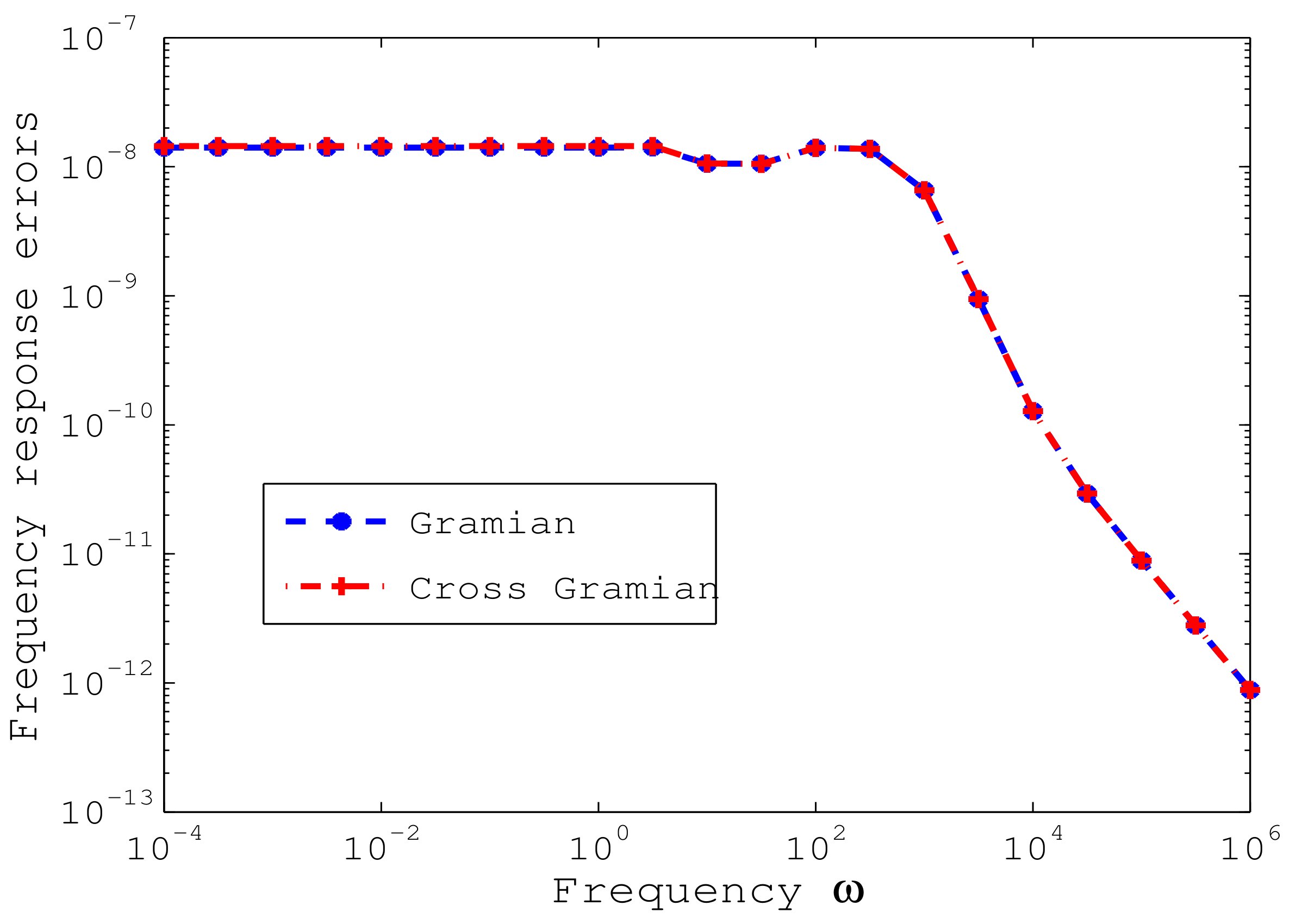
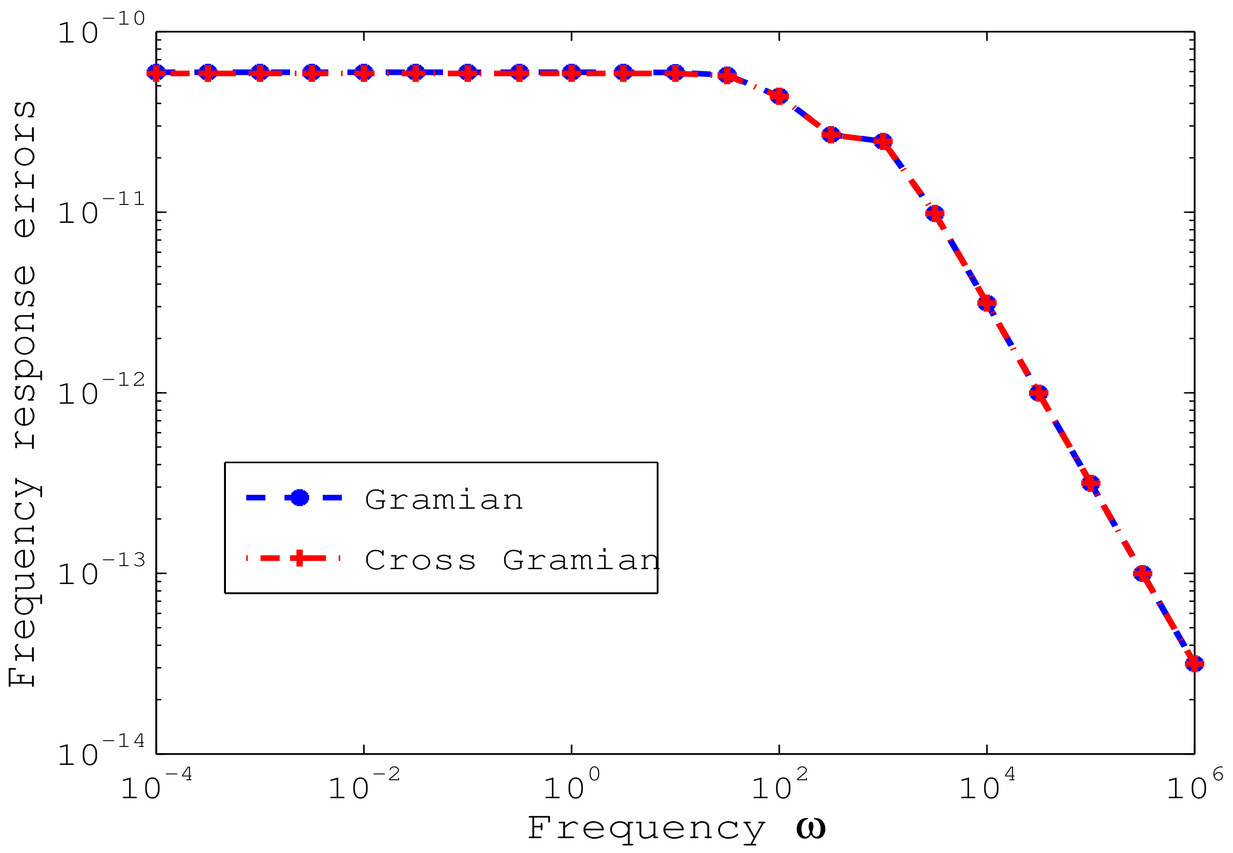
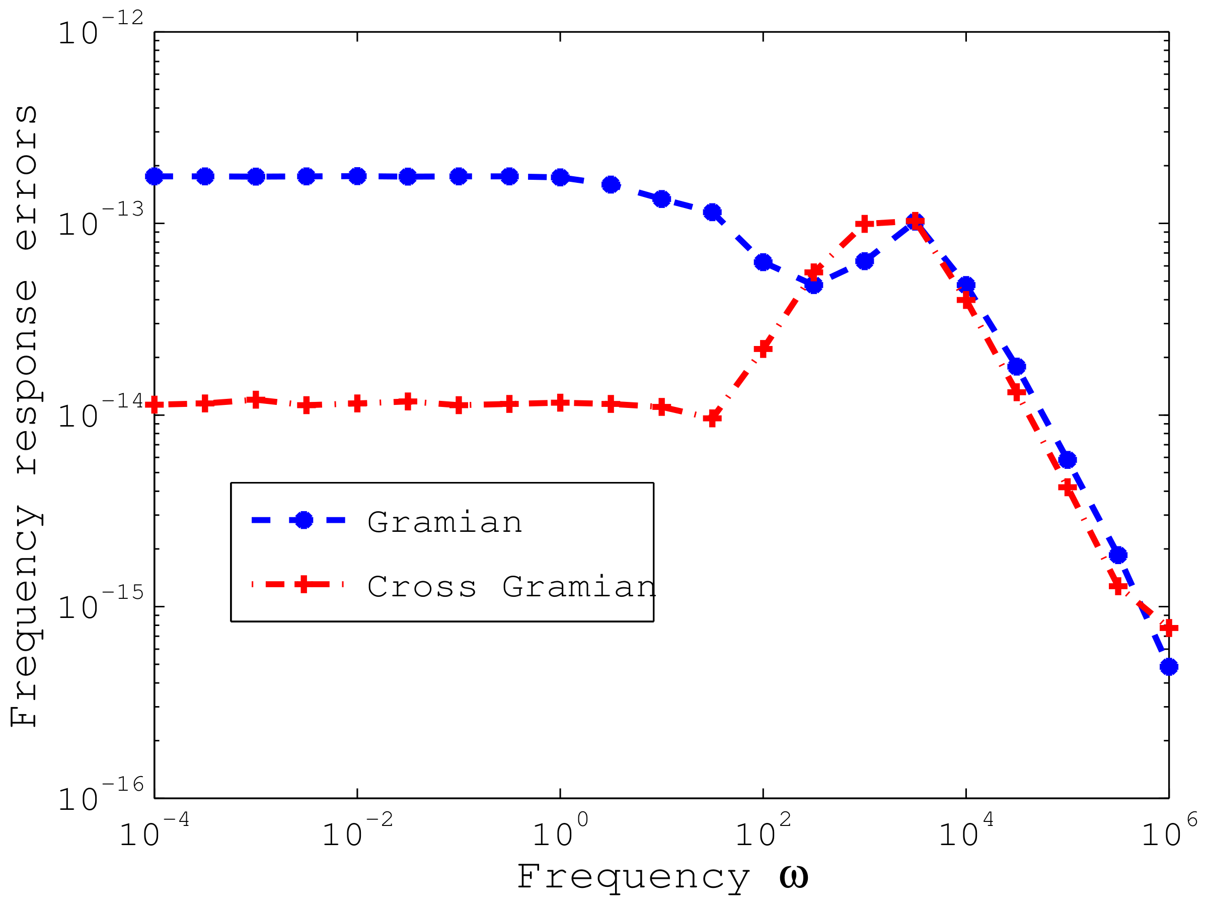
We first consider the SISO system, i.e., $m=p=1$. In this case, the analysis in Section 3 showed that the Gramian-based BFSR method and the cross-Gramian-based BFSR method should produce the same reduced system for the same reduced order. In Figure 1 and Figure 2, we present the absolute errors $|H\left(\mathrm{i}\omega \right)-\widehat{H}\left(\mathrm{i}\omega \right)|$ for these two methods in a frequency range $[{10}^{-4},{10}^6]$. From Figure 1 and Figure 2, it is clear that the errors for the Gramian-based BFSR method and the cross-Gramian-based BFSR method are almost indistinguishable.

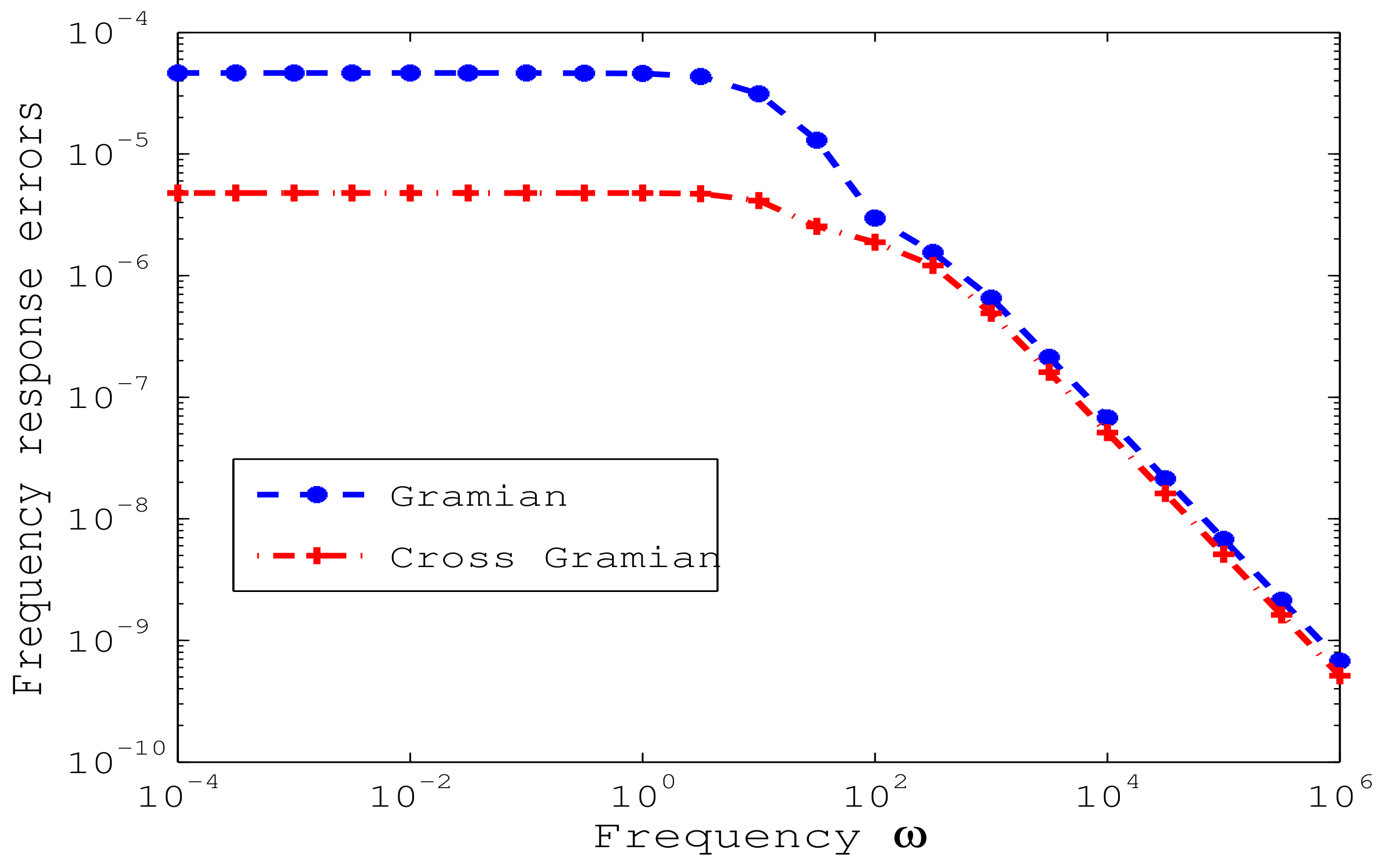
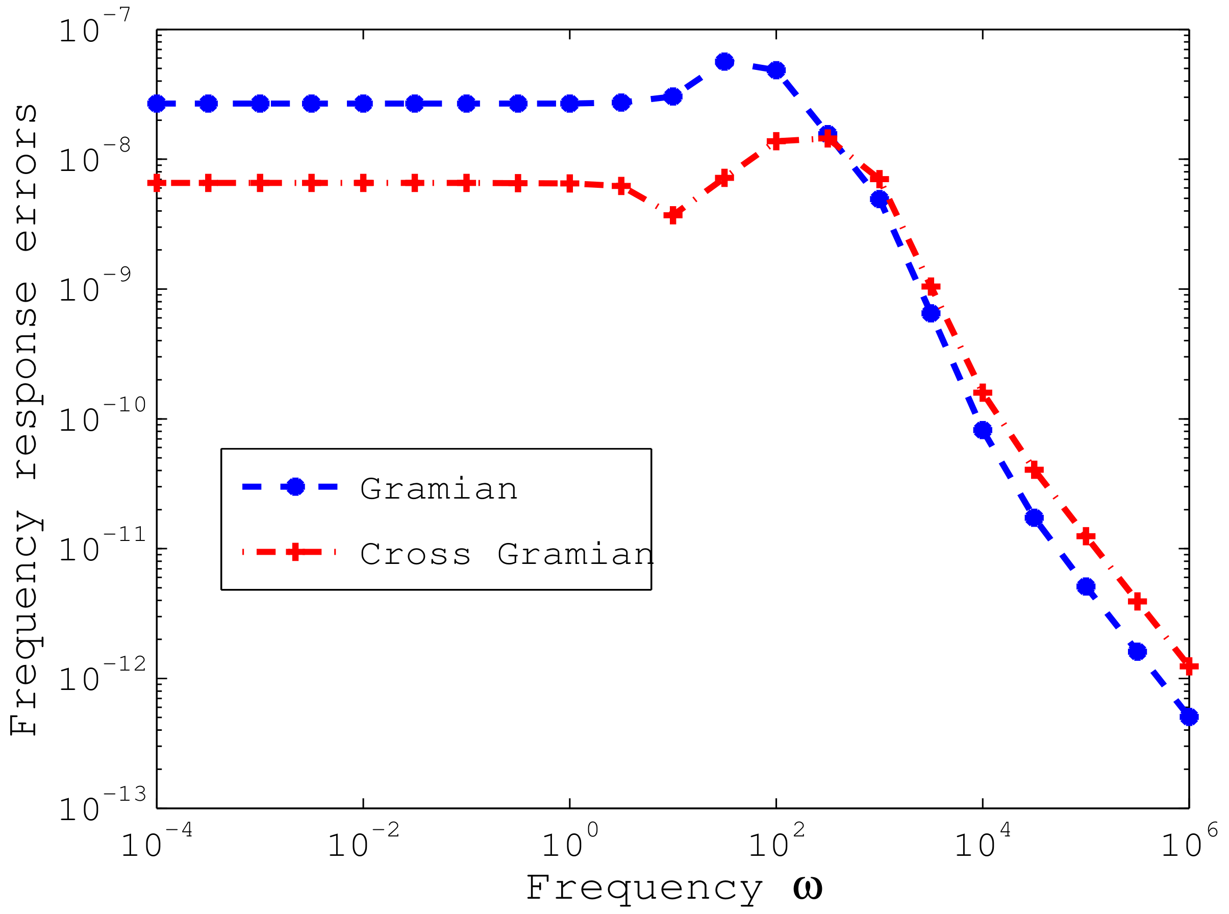
In the following experiment, we test the model order reduction of the square MIMO descriptor system with $m=p=2$. In the experiment, the first column and rows B and C are the same as those in the previous experiment. The second column of B is ${[1,1,\dots ,1]}^T$, whereas the second row of C is $[0,0,\dots ,0,1]$. Since the conditions of Theorems 4 and 5 do not hold in this case, the reduced systems generated by the Gramian-based BFSR method and the cross-Gramian-based BFSR method are usually different.

In Figure 3, Figure 4 and Figure 5, we display the $(1,1)-$th element of the absolute errors. We can see that the errors for the cross-Gramian-based BFSR method are fewer than those for the Gramian-based BFSR method in almost the whole frequency range $[{10}^{-4},{10}^2]$. This shows that the cross-Gramian-based BFSR method may generate more accurate reduced systems in low-frequency ranges.

It was shown in [16] that the cross-Gramian-based BFSR method can generate more accurate approximations for standard square nonsymmetric state-space systems since it computes the projection matrices $Q_L,Q_R$ from the cross Gramians. From the experimental results above, we can see that this maybe also holds true for square descriptor systems.

5. Conclusions

We have proposed a balancing-free square-root model reduction method based on cross Gramians for square descriptor systems in this paper. It is an extension of the balancing-free square root-model reduction method based on Gramians for square standard systems. This model reduction method can be implemented efficiently by exploiting the low-rank ADI and Smith methods for solving projected Sylvester equations. Numerical experiments illustrate the effectiveness of the cross-Gramian-based balanced truncation method.

References

- Alfke, D.; Feng, L.; Lombardi, L.; Antonini, G.; Benner, P. Model order reduction for delay systems by iterative interpolation. Int. J. Numer. Methods Eng. 2020, 122, 684–706. [Google Scholar]
- Benner, P.; Gugercin, S.; Willcox, K. A Survey of Projection-Based Model Reduction Methods for Parametric Dynamical Systems. SIAM Rev. 2015, 57, 483–531. [Google Scholar]
- Lu, K.; Yu, H.; Chen, Y.; Cao, Q.; Hou, L. A modified nonlinear POD method for order reduction based on transient time series. Nonlinear Dyn. 2015, 79, 1195–1206. [Google Scholar]
- Lu, K. Statistical moment analysis of multi-degree of freedom dynamic system based on polynomial dimensional decomposition method. Nonlinear Dyn. 2018, 93, 2003–2018. [Google Scholar]
- Allen, J.J. Micro Electro Mechanical System Design; CRC Press: Boca Raton, FL, USA, 2005. [Google Scholar]
- Günther, M.; Feldmann, U. CAD-based electric-circuit modeling in industry. i. mathematical structure and index of network equations. Surv. Math. Ind. 1999, 8, 97–129. [Google Scholar]
- Dai, L. Singular Control Systems; Lecture Notes in Control and Information Sciences; Springer: Berlin/Heidelberg, Germany, 1989; Volume 118. [Google Scholar]
- Moore, B.C. Principal component analysis in linear systems: Controllability, observability, and model reduction. IEEE Trans. Automat. Control 1981, 26, 17–32. [Google Scholar] [CrossRef]
- Liu, Y.; Anderson, B.D.O. Singular perturbation approximation of balanced systems. Int. J. Control 1989, 50, 1379–1405. [Google Scholar]
- Glover, K. All optimal Hankel-norm approximations of linear multivariable systems and their l∞-errors bounds. Int. J. Control 1984, 39, 1115–1193. [Google Scholar] [CrossRef]
- Benner, P.; Mehrmann, V.; Sorensen, D.C. (Eds.) Dimension Reduction of Large-Scale Systems; Lecture Notes in Computational Science and Engineering; Springer: Berlin/Heidelberg, Germany, 2005; Volume 45. [Google Scholar]
- Antoulas, A.C. Approximation of Large-Scale Dynamical Systems; SIAM: Philadelphia, PA, USA, 2005. [Google Scholar]
- Antoulas, A.C.; Sorensen, D.C.; Gugercin, S. A survey of model reduction methods for large-scale systems. Contemp. Math. 2001, 280, 193–219. [Google Scholar]
- Bai, Z. Krylov subspace techniques for reduced-order modeling of large-scale dynamical systems. Appl. Numer. Math. 2002, 43, 9–44. [Google Scholar]
- Freund, R.W. Model reduction methods based on krylov susbspace. Acta Numer. 2003, 12, 267–319. [Google Scholar]
- Baur, U.; Benner, P. Cross-gramian based model reduction for data-sparse systems. Electr. Trans. Numer. Anal. 2008, 31, 256–270. [Google Scholar]
- Sorensen, D.C.; Antoulas, A.C. The sylvester equation and approximate balanced reduction. Linear Algebra Appl. 2002, 352, 671–700. [Google Scholar] [CrossRef] [Green Version]
- Stykel, T. Gramian-based model reduction for descriptor systems. Math. Control Signals Systems 2004, 16, 297–319. [Google Scholar] [CrossRef]
- Low-rank iterative methods for projected generalized Lyapunov equations. Elect. Trans. Numer. Anal. 2008, 30, 187–202.
- Varga, A. Efficient minimal realization procedure based on balancing. In Proceedings of the IMACS/IFAC Symposium on Modelling and Control of Technological Systems, Lille, France, 7–10 May 1991; Volume 2, pp. 42–47. [Google Scholar]
- Stykel, T. Analysis and Numerical Solution of Generalized Lyapunov Equations. Ph.D. Thesis, Technische Universität Berlin, Berlin, Germany, 2002. [Google Scholar]
- Gantmacher, F. Theory of Matrices; Chelsea: New York, NY, USA, 1959. [Google Scholar]
- Cobb, D. Controllability, observability, and duality in singular systems. IEEE Trans. Automat. Control 1984, 29, 1076–1082. [Google Scholar]
- Yip, E.L.; Sincovec, R.F. Solvability, controllability and observability of continuous descriptor systems. IEEE Trans. Automat. Control 1981, 26, 702–707. [Google Scholar]
- Golub, G.H.; Loan, C.F.V. Matrix Computations, 3rd ed.; Johns Hoplins University Press: Baltimore, MD, USA, 1996. [Google Scholar]
- Mehrmann, V.; Stykel, T. Balanced truncation model reduction for large-scale systems in descriptor form. In Dimension Reduction of Large-Scale Systems; Benner, P., Mehrmann, V., Sorensen, D., Eds.; Lecture Notes in Computational Science and Engineering; Springer: Berlin/Heidelberg, Germany, 2005; Volume 45, pp. 83–115. [Google Scholar]
- Li, J.; White, J. Low rank solution of lyapunov equations. SIAM J. Matrix Anal. Appl. 2002, 24, 260–280. [Google Scholar]
- Penzl, T. A cyclic low-rank smith method for large sparse lyapunov equations. SIAM J. Sci. Comput. 2000, 21, 1401–1418. [Google Scholar]
- Fernando, K.; Nicholson, H. On the structure of balanced and other principal representations of SISO systems. IEEE Trans. Automat. Control 1983, 28, 228–231. [Google Scholar]
- Benner, P.; Li, R.; Truhar, N. On the ADI method for Sylvester equations. J. Comput. Appl. Math. 2009, 233, 1035–1045. [Google Scholar]
- Stykel, T. Balanced truncation model reduction for semidiscretized Stokes equation. Linear Algebra Appl. 2006, 415, 262–289. [Google Scholar]
- Lin, Y.; Bao, L. The projected generalized Sylvester equations: Numerical solution and applications. WSEAS Trans. Math. 2016, 15, 83–95. [Google Scholar]
Figure 1.
The frequency response errors of the SISO reduced system generated by the Gramian-based BFSR method and the cross-Gramian-based BFSR method with the reduced order .
Figure 2.
Figure 3.
The frequency response errors of the MIMO reduced system generated by the Gramian-based BFSR method and the cross-Gramian-based BFSR method with the reduced order .
Figure 4.
Figure 5.
Publisher’s Note: MDPI stays neutral with regard to jurisdictional claims in published maps and institutional affiliations. |
© 2022 by the author. Licensee MDPI, Basel, Switzerland. This article is an open access article distributed under the terms and conditions of the Creative Commons Attribution (CC BY) license (https://creativecommons.org/licenses/by/4.0/).
Share and Cite
MDPI and ACS Style
Lin, Y. Cross-Gramian-Based Model Reduction for Descriptor Systems. Symmetry 2022, 14, 2400. https://doi.org/10.3390/sym14112400
AMA Style
Lin Y. Cross-Gramian-Based Model Reduction for Descriptor Systems. Symmetry. 2022; 14(11):2400. https://doi.org/10.3390/sym14112400
Chicago/Turabian StyleLin, Yiqin. 2022. "Cross-Gramian-Based Model Reduction for Descriptor Systems" Symmetry 14, no. 11: 2400. https://doi.org/10.3390/sym14112400
Note that from the first issue of 2016, this journal uses article numbers instead of page numbers. See further details here.