A Low-Cost Algorithm for Uncertainty Quantification Simulations of Steady-State Flows: Application to Ocular Hemodynamics

Abstract

An algorithm for the calculation of steady-state flowing under uncertain conditions is introduced in this work in order to obtain a probabilistic distribution of uncertain problem parameters. This is particularly important for problems with increased uncertainty, as typical deterministic methods are not able to fully describe all possible flow states of the problem. Standard methods, such as polynomial expansions and Monte Carlo simulations, are used for the formation of the generalized problem described by the incompressible Navier-Stokes equations. Since every realization of the uncertainty parameter space is coupled with non-linear terms, an incremental iterative procedure was adopted for the calculation. This algorithm adopts a Jacobi-like iteration methodology to decouple the equations and solve them one by one until there is overall convergence. The algorithm was tested in a typical artery geometry, including a bifurcation with an aneurysm, which consists of a well-documented biological flow test case. Additionally, its dependence on the uncertainty parameter space, i.e., the inlet velocity distribution, the Reynolds number variation, and parameters of the procedure, i.e., the number of polynomial expansions, was studied. Symmetry exists in probabilistic theories, similar to the one adopted by the present work. The results of the simulations conducted with the present algorithm are compared against the same but unsteady flow with a time-dependent inlet velocity profile, which represents a typical cardiac cycle. It was found that the present algorithm is able to correctly describe the flow field, as well as capture the upper and lower limits of the velocity field, which was made periodic. The comparison between the present algorithm and the typical unsteady one presented a maximum error of ≈2% in the common carotid area, while the error increased significantly inside the bifurcation area. Moreover, “sensitive” areas of the geometry with increased parameter uncertainty were identified, a result that is not possible to be obtained while using deterministic algorithms. Finally, the ability of the algorithm to tune the parameter limits was successfully tested.

1. Introduction

The evaluation of uncertainty is fundamental to the quantification of the accuracy of expected values in both theoretical and experimental studies. Many problems in natural sciences and engineering are also rife with sources of uncertainty. Complex systems are designed using computational models that are based on both a mathematical description of the physics and numerical algorithms that solve the resulting set of (partial differential) equations (PDE), e.g., finite element (FE) models [1,2,3,4]. The uncertainty of a problem can be attributed to any of its variables. This practically means that sources of uncertainty could be various variables in seemingly very different problems, from varying viscosity or temperature in nanofluid studies [5,6,7,8], to varying velocities in ocular hemodynamic studies, such as the present one. The application of computational fluid dynamics (CFD) methods has become quite popular during the past decades in many scientific areas, including bioengineering and hemodynamics. One of the major advantages of the CFD methods that makes them so attractive in these areas of research is their capability to sufficiently represent the physics of coupled systems. The results of CFD numerical experiments can seriously assist the decision-making process in real-life medical applications or clinical trials [9,10,11,12,13,14]. More specifically, hemodynamic flows that can be found in the human body consist of a great area of CFD applications. In most of the existing human hemodynamic flow studies, there is no parameter space given, rather a set of fixed values is considered. In this way, these studies do not take into account the actual parameter values of the problem that they attempt to solve, as parameter values of human hemodynamic flows may vary vastly, and in most cases are patient-specific. Additional sources of uncertainty can arise due to nature of numerical simulations. This type of uncertainty may arise due to physics or geometry complexities, or when initial and boundary data are not fully prescribed. So, these conditions present uncertainties, which are omnipresent in all modeling approaches, making it impossible to carry out a deterministic study [15]. A very good approach to overcoming the problems posed by this type of flow is the application of probabilistic analysis. This way, the output will be based on the uncertainty of input data, rather than on a fixed set of parameter values. The combination of uncertainty analysis with probabilistic methods can provide very interesting and helpful results, especially in the case of human hemodynamic flows, where patient-specific data pose extra difficulties [14].

The uncertainty quantification (UQ) algorithm seems to be an ideal candidate in order to tackle the above-mentioned problems. Numerical simulations with the (UQ) algorithm may include as input a parameter space of variables, such as flow velocity, blood pressure, and the geometry of the arterial and vascular networks. The quantification of the above-mentioned parameters will lead to more precise results, which can be better compared to experimental or even clinical ones [12,13,14,15].

Constructing a model that successfully represents human hemodynamic flows in the vascular network, both arterial and venular, under uncertain conditions, is a very demanding process, mostly due to the variability of the physical parameters used in the numerical models, the uncertainties occurring from a lack of information linked to the boundary conditions and the considerable unavailability of patient-specific clinical data. An ocular vascular system is characterized by both vast complexity and extremely small dimensions. The great majority of the existing research applications of UQ in biomedical sciences refer to a large-scale arterial, cardiovascular, and aortic network, in anatomical, orthopedic structures, implant design parameters, neural networks, and brain structures [16]. In large-diameter vessels, the non-Newtonian characteristics of the blood are less important and the blood can be represented by a Newtonian fluid model with a constant viscosity factor, without creating a significant error. Blood can also be considered an incompressible fluid, i.e., the density of the blood is considered constant with a value of 1060 kg/m³.

Another aspect that should be highlighted is the need to develop UQ mathematical models, such as a useful tool for the detection and quantification of ocular hemodynamic flow disorders. It is widely believed that ocular hemodynamic flow disorders are extremely important regarding the manifestation of underlying pathology not only in the eye, but in the human body in general. Disturbances in the ocular hemodynamic flows are not only associated with eye diseases (age-related macular degeneration, uveitis, retinopathy, glaucoma) but usually testify to the existence of more general underlying diseases in the human body such as hypertension, diabetes, and multiple sclerosis.

It should also be emphasized that the eye vessels are characterized by the peculiarity of being the only vessels of the human body that are accessible (non-invasively and macroscopically) through simple ophthalmoscopy (by fundus camera) and hemodynamic measurements of the macro- and micro-circulation (by optical coherence tomography—OCT). Traditionally, more detailed and thorough measurements can be obtained post-mortem (from human eyes), from similar animal eyes, or finally from statistical studies in population groups. It can be easily understood that all three of these methods are characterized by inherent disadvantages.

There are additional reasons for the necessity of modeling. In pathological conditions, some of the mechanisms of vascular regulation may be affected, with the result that retinal oxygenation is disturbed. Then, a discrepancy is observed in the international scientific literature regarding the response of the vascular network to changes in oxygen demand. Moreover, contradictory clinical observations sometimes occur due to the numerous influencing factors, including arterial blood pressure and vascular regulation, which affect the relationship between intra-ocular pressure (IOP) and ocular hemodynamics. Finally, mathematical modeling can be used to explore the complex relationship between these factors and to interpret the results of clinical studies. By the term “mathematical modeling of hemodynamic flows”, we mean, (i) the most accurate representation of the existing geometric structures of the vascular network, (ii) the most realistic fluid-mechanical description of the physical processes taking place, as well as (iii) the most representative description of the interaction between them. Potentially successful modeling could provide a better understanding and interpretation of the functions and phenomena.

Although ophthalmic anatomy and physiology seem to be quite suitable areas for implementing the UQ concept and formalism, there is a complete lack of relevant articles in the research literature. Even the few existing articles that enable the term “Uncertainty Quantification” do not adopt the formal depiction of the so-called mathematical method. The main and governing characteristic of ocular hemodynamic flows is the micro-scale of the vascular network, both arterial and venular. This implies that someone can safely assume that the existing values of blood flow velocity and Reynolds number are rather low. This fact is verified by clinical measurements [14,17]. Subsequently, the blood flow is laminar and approached according to the typical incompressible Navier-Stokes equations. Blood is assumed to be either a Newtonian or non-Newtonian incompressible fluid. Ocular hemodynamic flows are widely and thoroughly studied in terms of mathematical modeling and computational fluid dynamics [18,19,20,21,22,23,24,25,26,27,28,29], there are no research approaches that enable a wide, full, and extensive implementation of UQ.

This study focuses on developing a low-cost finite element (FE) [9,10,11,12,13,14,15] algorithm for the simulation of steady-state flows under uncertainty quantification of the implicated physical properties. The main goal of the algorithm is to obtain fast results of the probabilistic distribution of the model outputs. The suitability and the utility of the algorithm are tested on the well-documented case of a realistic artery model, including a bifurcation and aneurysm area. The results of the model are compared against the results of unsteady simulations, computed on the same geometry by solving the typical Navier-Stokes equation. In the case of the unsteady simulation, a time-dependent inlet velocity profile was employed, which was made periodic in order to represent a typical cardiac cycle. The ability of the present algorithm to successfully describe the probabilistic distribution of the model outputs was also demonstrated. Finally, relevant conclusions were extracted and future perspectives are outlined.

2. Materials and Methods

Quantification of fluid quantities, such as momentum and heat transfer flow under uncertain conditions, is a natural choice for modern scientists to successfully predict typical experimental or field measurement results where many parameters are difficult to remain constant. In the typical uncertainty quantification (UQ) formulation of the Navier-Stokes equation, parameters, such as boundary conditions, differences in the geometry of the domain, density, and temperature fluctuations, and possible measurement fluctuations may be sources of uncertainty. In the UQ method [30,31], all sources of uncertainty are parameterized in a single parameter space P and the governing equations need to be solved simultaneously in P space. This is a fundamental difficulty of the UQ method as compared to the typical deterministic fluid flow simulations. The already extensive system of discrete equations, of a single parameter set, needs to be solved now coupled together in a system of equations multiple to P [30,31].

Under the UQ concept, and by adopting the polynomial chaos (PC) [32,33,34,35] representation of all field variables in the flow, namely the pressure, p, and the velocity vector, $\mathbf{u}$ (and possible other quantities such as temperature and temperature-dependent fluid properties and boundary conditions introduced in the non-dimensionalization of the equations, i.e., the Reynolds, Prandtl, Rayleigh Numbers), can be expanded as [36]:

$$p\left(\mathbf{x}\right)=\sum _{i=0}^P{p}_i\left(\mathbf{x}\right){\mathrm{\Psi }}_i$$

(1)

$$\mathbf{u}\left(\mathbf{x}\right)=\sum _{i=0}^P{\mathbf{u}}_i\left(\mathbf{x}\right){\mathrm{\Psi }}_i$$

(2)

where $\mathbf{x}$ denotes the spatial domain, and ${\mathrm{\Psi }}_i$ are the functionals of the PC basis.

The typical incompressible transient Navier-Stokes equations can be formulated for the field variables in $k\in (0,P)$ as [36]:

$$\begin{array}{ccc}\hfill \nabla ·{\mathbf{u}}_k& =& 0\hfill \end{array}$$

(3)

$$\begin{array}{ccc}\hfill \frac{\partial {\mathbf{u}}_k}{\partial t}+\sum _{i=0}^P\sum _{j=0}^P{C}_{ijk}\left({\mathbf{u}}_i·\nabla \right){\mathbf{u}}_j& =& -\nabla p_k+\frac{1}{R{e}_k}\Delta {\mathbf{u}}_k+f_k\hfill \end{array}$$

(4)

where the indexes $k,i,j=0\dots P$, t is the time, $R{e}_k=u_{inlet}D/{\nu }_k$ is the Reynolds number based on the mean characteristic velocity at the inlet $u_{inlet}$, the characteristic length D and the kinematic viscosity ${\nu }_k$, f is a potential forcing term due to gravity or other forces, and finally, the multiplication tensor is given by:

$$C_{ijk}\equiv \frac{〈{\mathrm{\Psi }}_i{\mathrm{\Psi }}_j{\mathrm{\Psi }}_k〉}{〈{\mathrm{\Psi }}_k{\mathrm{\Psi }}_k〉}$$

(5)

Obviously, the non-linear term in the momentum equation couples the $P+1$ equations (4), however, the simultaneous solution of an approximation system of size: $4\times (P+1)\times$ (the size of spatial discretization) × (the number of the time-steps of the temporal discretization) is very expensive. The solution of this large system of equations is unavoidable in the case of transient or time-dependent flows; however, in some cases, the flow may result in stationarity or even steady-state (both in laminar or turbulent modeling with RANS methods). Even in the hemodynamic flow of our interest here, the time-dependent blood inflow velocity can be considered to have a mean and a fluctuating part that could be represented as $P+1$ different flow instances ensemble together in a steady-state UQ system. The cost of the solution of the final system in the case of steady-state conditions may be reduced.

Although algorithms for the UQ of unsteady flows can be found even in textbooks (see for example [36]), no particular method is reported so far for the UQ solution of the steady-state Navier-Stokes equations, except using their unsteady formulation and repeatedly solve them for all time steps until stationarity. In the present work, an iterative algorithm similar to Jacobi or Gauss–Seidel methods is presented to treat the non-linear terms of the steady-state UQ equations.

Under steady-state conditions, the coupled system of Equations (3) and (4) may read as:

$$\begin{array}{ccc}\hfill \nabla ·{\mathbf{u}}_k& =& 0\hfill \end{array}$$

(6)

$$\begin{array}{ccc}\hfill \sum _{i=0}^P\sum _{j=0}^P{C}_{ijk}\left({\mathbf{u}}_i·\nabla \right){\mathbf{u}}_j& =& -\nabla p_k+{\frac{1}{Re}}_k\Delta {\mathbf{u}}_k+f_k\hfill \end{array}$$

(7)

For every equation k, only the non-linear term is coupled and may be split in the form:

$$\begin{array}{ccc}\hfill \sum _{i=0}^P\sum _{j=0}^P{C}_{ijk}\left({\mathbf{u}}_i·\nabla \right){\mathbf{u}}_j& =& \sum _{i=0}^{P,i\ne k}\sum _{j=0}^{P,j\ne k}{C}_{ijk}\left({\mathbf{u}}_i·\nabla \right){\mathbf{u}}_j+C_{kkk}\left({\mathbf{u}}_k·\nabla \right){\mathbf{u}}_k\hfill \end{array}$$

(8)

Thus, introducing Equation (8) into Equation (7), the governed equations can read as:

$$\begin{array}{ccc}\hfill \nabla ·{\mathbf{u}}_k& =& 0\hfill \end{array}$$

(9)

$$\begin{array}{ccc}\hfill C_{kkk}\left({\mathbf{u}}_k·\nabla \right){\mathbf{u}}_k+\nabla p_k-\frac{1}{R{e}_k}\Delta {\mathbf{u}}_k-f_k& =& -f_{UQ}^k\hfill \end{array}$$

(10)

with,

$$\begin{array}{c}\hfill f_{UQ}^k=\sum _{i=0}^{P,i\ne k}\sum _{j=0}^{P,j\ne k}{C}_{ijk}\left({\mathbf{u}}_i·\nabla \right){\mathbf{u}}_j\end{array}$$

(11)

The system of Equations (9) and (10) can be solved, as usual, with the use of Newton’s method (and also any other method available for the solution of the steady-state Navier-Stokes equations, such as the SIMPLE method or the artificial compressibility method) with an iteration-uncoupled formulation of the non-linear terms. Thus, in the proposed algorithm, a Jacobi-like method is used iteratively between the $P+1$ equation systems of the entire UQ problem for the solution of each k equation set of the system Equations (9) and (10) separately (and not coupled). The non-linear term $f_{UQ}^k$ will be treated as a source term, where its value can be evaluated from the old iteration (such as in the Jacobi method), $n-1$, or from previous solutions in the same iteration (such as in the Gauss–Seidel method), n, as:

$$\begin{array}{ccc}\hfill f_{UQ}^k& =& \sum _{i=0}^{k-1}\sum _{j=0}^{k-1}{C}_{ijk}\left({\mathbf{u}}_i^n·\nabla \right){\mathbf{u}}_j^n+\sum _{i=k+1}^P\sum _{j=k+1}^P{C}_{ijk}\left({\mathbf{u}}_i^{n-1}·\nabla \right){\mathbf{u}}_j^{n-1}\hfill \end{array}$$

(12)

The Monte Carlo method is used for the sampling of the uncertain parameters i.e., the inlet velocity fluctuations and the Reynolds number fluctuation due to viscosity differences of the problem using the pseudo-random Hammersley method [2]. For different scenarios that are presented in Section 3, the parameters under uncertainty are allowed to vary from $25\%$ up to $100\%$ of their mean values, while three different $Re$ cases are examined, $Re=1,5$ and 10. The present $Re$ values were selected, as they corresponded to typical ocular hemodynamics values. The sample parameter space for each problem was selected to vary between $P=10$ to 50. Normal distribution was selected for the uncertain inlet velocity boundary condition and uniform distribution for the Reynolds number. Figure 1 is showing the $u_{k,inlet}$ and $R{e}_k$ parameter space for $P=10$, 20 and 50 for the indicative distribution of the cases with a standard deviation of $25\%$ in the inlet velocity and the Reynolds number around the mean value of $Re=10$.

The Fenics project was used to provide the automated solution of the Navier-Stokes equations with the discretization of non-linear equations based on the finite element method [3,4]. The Taylor–Hood [1] $(P1-P2)$ stable finite element formulation for the pressure and velocity, respectively, was selected for the N triangular cells that cover the artery vessel domain. A typical two-dimensional vessel geometry was used for this purpose, including the additional complexity of a bifurcation and an aneurysm (Figure 2). The main diameter of the geometry was selected to be equal to $D=200$μm, thus representing a typical ocular artery diameter. 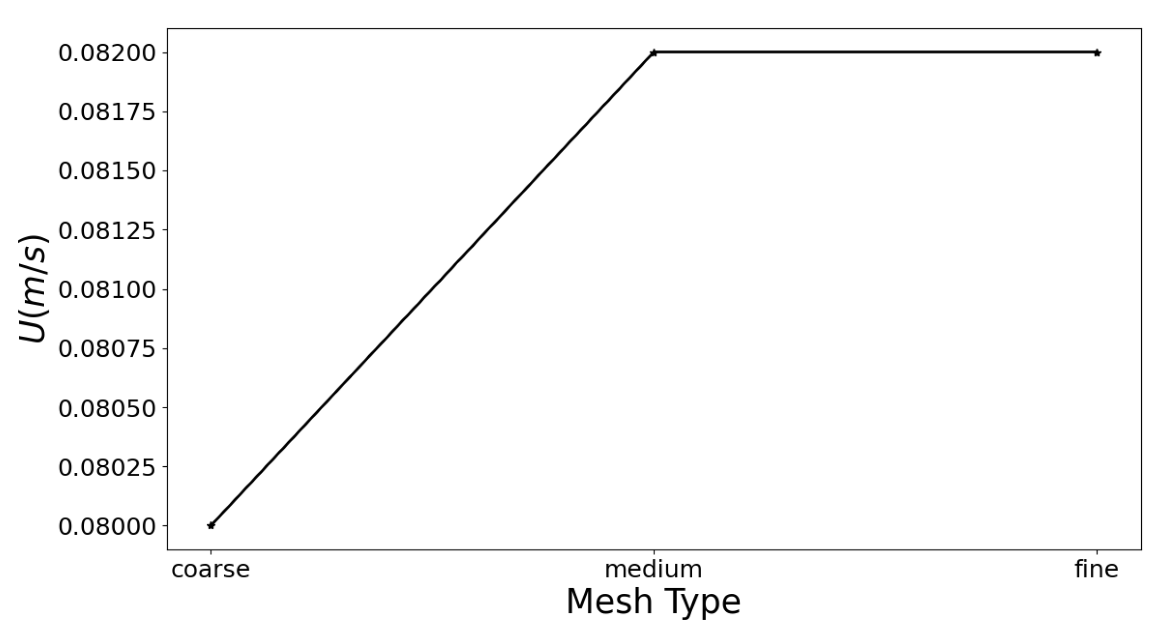An indicative mesh distribution is presented in (Figure 2). As far as the meshing strategy is concerned, an unstructured mesh approach was selected, while a mesh independence study was conducted prior to the simulations. The higher $Re=10$ case was selected in order to certify the ability of the mesh to correctly resolve the flow field. For this purpose, the velocity was computed at the center of the geometry for three different mesh size cases. The results of the maximum velocity for the different mesh size cases are presented in Figure 3, where the medium mesh size can be considered adequate in order to correctly represent the flow field. The model is also tested against the well-documented case of a realistic artery model [37], including a bifurcation and aneurysm area.

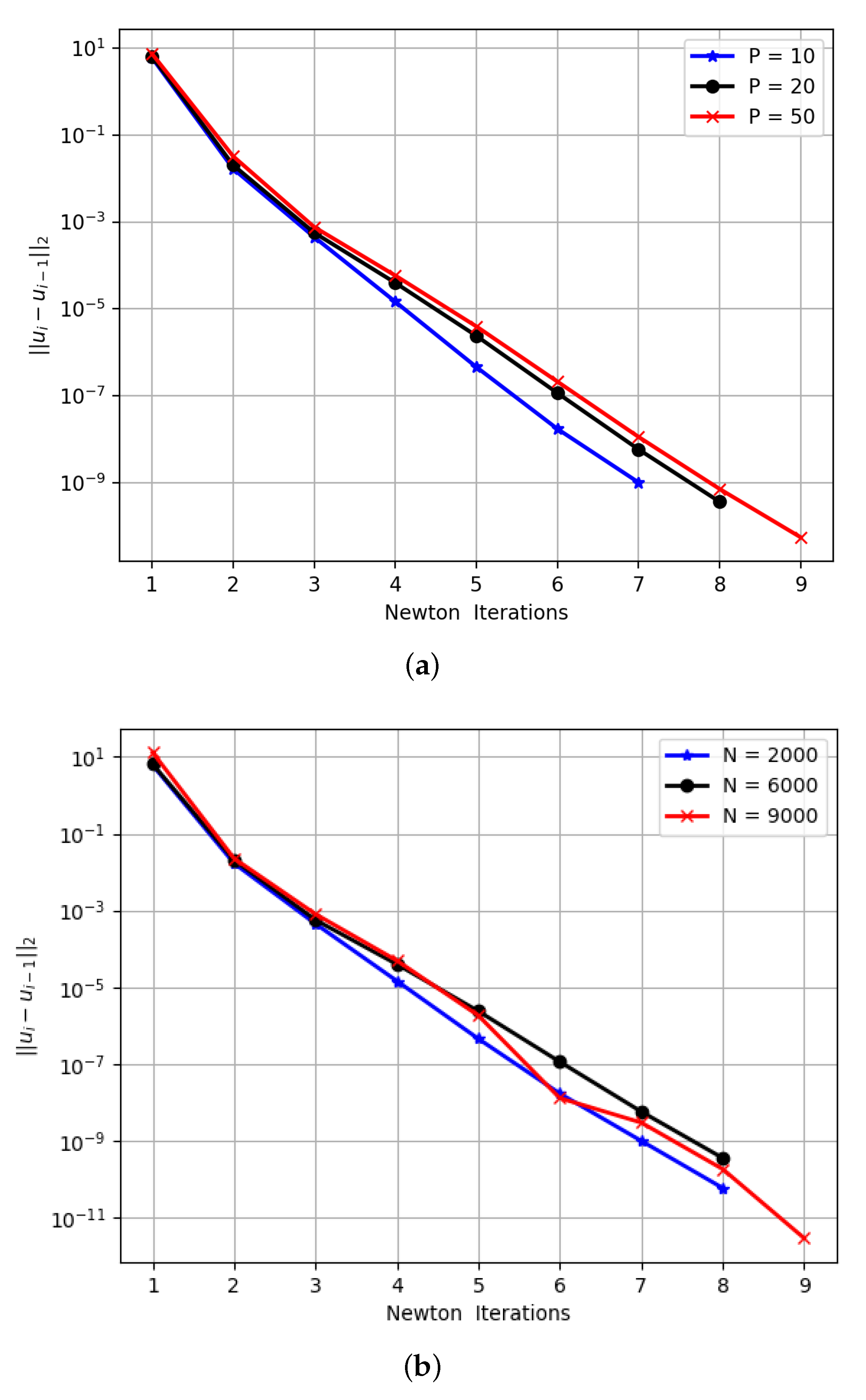
The algorithm starts from arbitrary initial values of the $p_k^0$ and $u_k^0$ quantities in all P systems of equations. Each system is solved from these initial conditions and with UQ forcing, $f_{UQ}^1$ that is based also on the arbitrary initial values of $u_k^0$. When all systems are solved separately, the algorithm starts again from the first system, and the quantities $p_k^1$ and $u_k^1$ of all other systems and repeated till convergence. The maximum error between the systems solutions for all iterations is presented in Figure 4a for $P=10,20$, and 50 for a mesh size of $N=6000$. For the lower samples of $P=10$, just 7 iterations are adequate to reduce the maximum error to less than ${10}^{-9}$, while as P increases to 50 only two more iterations are needed for an even lower error. The effect of mesh size N in the convergence of the algorithm is shown in Figure 4b. As N increases from 2000 to 9000 triangles only one additional iteration, from 8 to 9, is needed to decrease the error to less than ${10}^{-11}$. Thus, for all the simulations in the next section, a mesh of $N=6000$ and $P=20$ is selected.

The results of the current algorithm simulations were compared against unsteady Navier-Stokes simulations of the same geometry, where a time-dependent inlet velocity profile was implemented in order to mimic the cardiac cycle, Figure 5, the mean and the fluctuating part of this function is used also in the UQ velocity inlet distributions. Before comparison, the unsteady simulations have run for at least four periods.

3. Results and Discussion

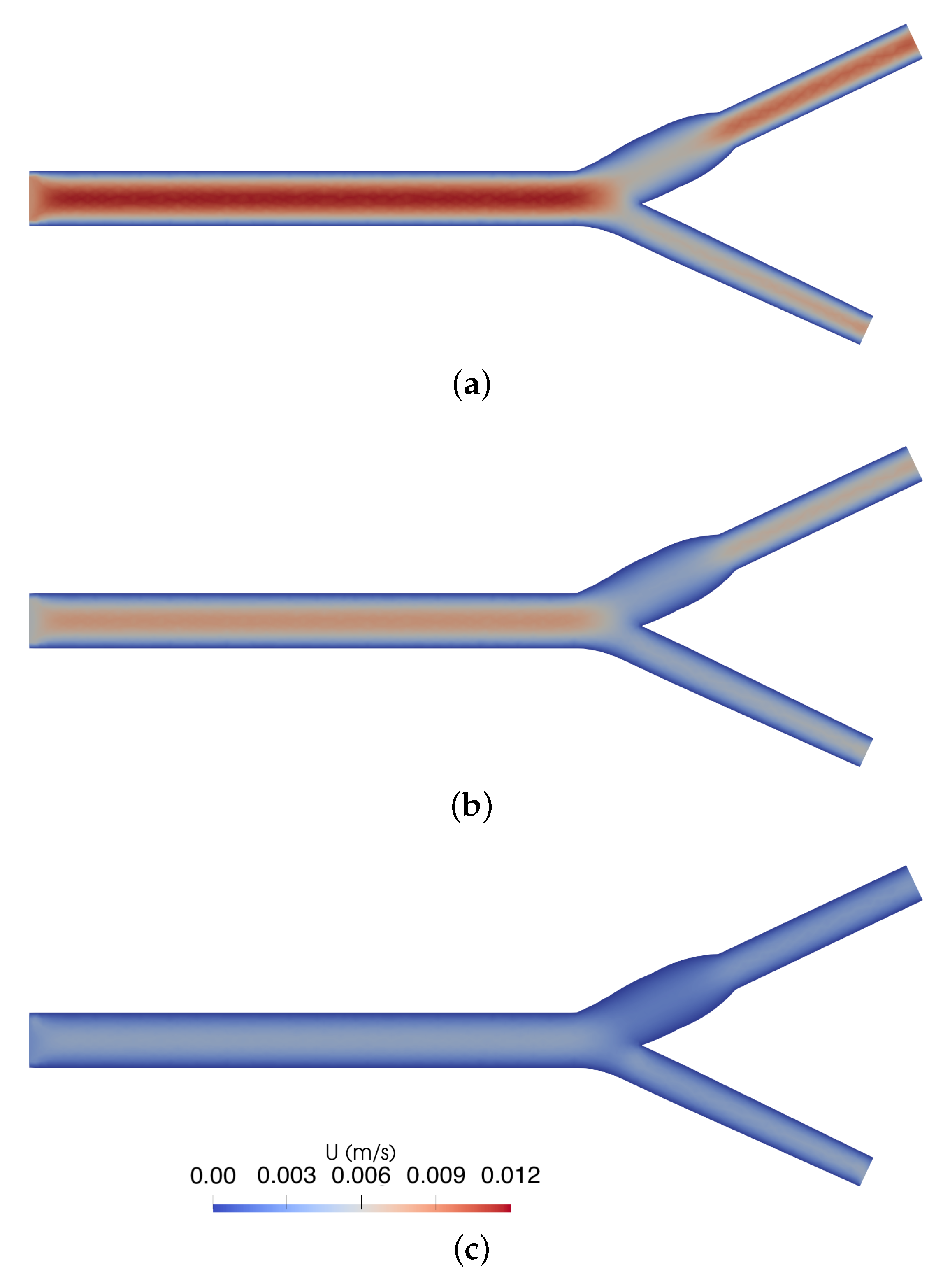
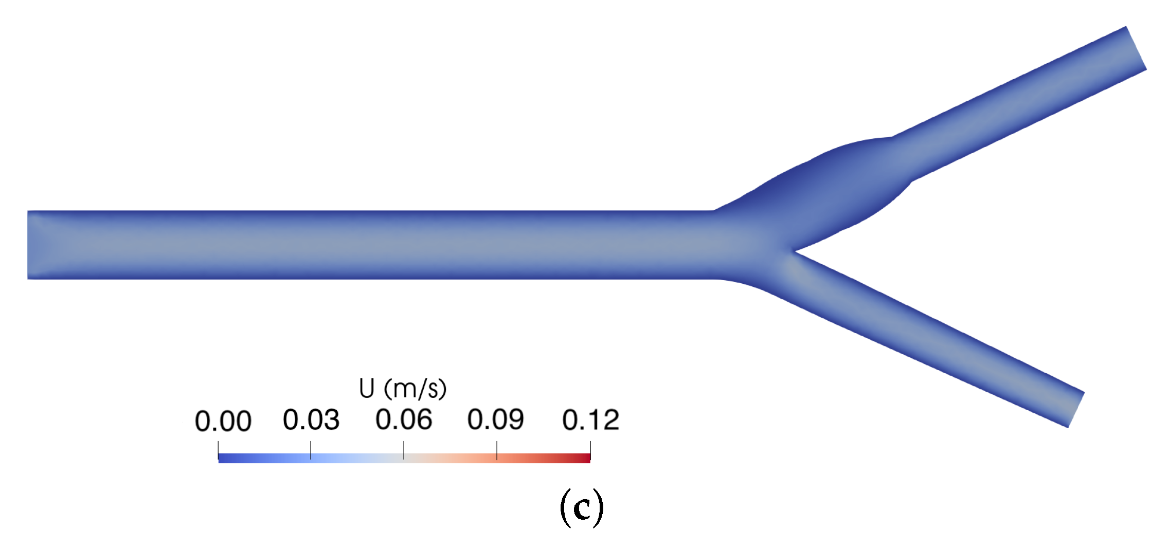
The flow field produced by the UQ algorithm for $P=20$ was initially studied through the velocity magnitude contours of $Re=$ 1 and 10, as shown in Figure 6 and Figure 7, respectively. More specific, velocity magnitude contours are presented for their maximum (upper), mean (middle) and minimum (bottom) distributions in Figure 6 and Figure 7 as calculated by the UQ algorithm for the two different Reynolds number cases and for standard deviation of the inlet velocity and the $R{e}_k$ equal to $50\%$. From these plots, the Figure 6b velocity distribution is the more possible to occur for $Re=1$ and almost corresponds to the mean velocity of the unsteady simulation. The Figure 6a,c, are the maximum and minimum stages the velocity could be found in this flow according to the UQ concept. Both situations are not very possible to occur or to appear for long in the flow but only in the extremes of the inlet velocity of Figure 5.

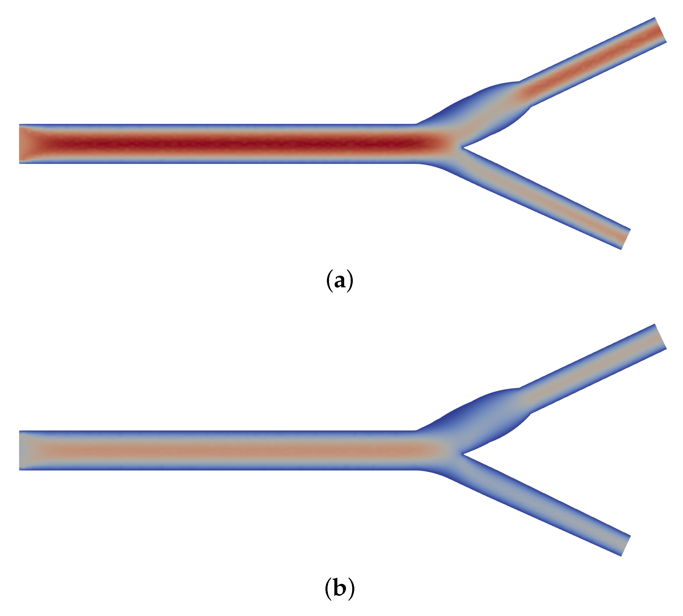
One advantage of the UQ methodology is the ability to capture possible sensitive areas in the flow field with unusual dynamics. This is the case of Figure 7a after the bifurcation, where the velocity field of the higher $Re$ case becomes clearly more unstable as compared to the lower $Re$ case. This flow field instability is the reflection of higher uncertainty, a characteristic that is completely absent in the classic unsteady Navier-Stokes simulations.

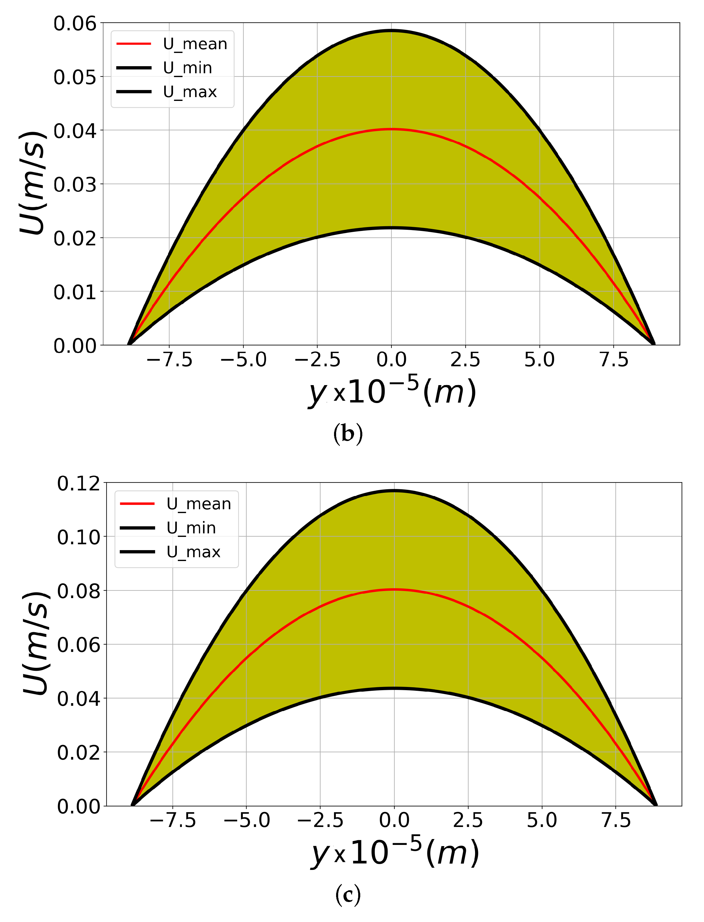
A better understanding of the results that are produced by the UQ algorithm can be obtained by examining the velocity profiles of the aforementioned scenarios. The mean streamwise velocity profiles obtained by the UQ algorithm simulations are plotted in Figure 8 for all three $Re$ cases, along with the upper and lower limits of streamwise velocity, which were calculated according to the standard deviation value of $50\%$. All velocity profiles were measured at the same positions, at the center of the geometry prior to the bifurcation for $L=1.7\mathsf{\mu }$m, and plotted versus Y-axis. The yellow highlighted area denotes the space between the min and max limits of velocity. The UQ algorithm simulation results suggest that the flow field is described correctly, as parabolic profiles were obtained in all cases. The colored area is the space where all possible velocities of the flow will be found, while the red line is the mean and most possible velocity distribution to occur.

In order to validate the UQ algorithm, the velocity profile of the common artery geometry was plotted against a well-documented case of the same geometry [38]. In Figure 9, velocity profiles of the present study and the one of Gjisen et al. [38] are compared in the center of the geometry before the bifurcation, for normalized velocity and diameter, presenting excellent agreement. Furthermore, unsteady simulations were conducted for the same Reynolds numbers and their results were compared against the present UQ algorithm results. In order to keep this comparison more comprehensive, the difference between the two types of simulations is presented as an error percentage in

Table 1. Error percentage calculated between velocity curves of UQ algorithm and unsteady Navier-Stokes simulations, at the center of the geometry prior to the bifurcation. The error percentage is presented for cases of $Re=1,5$, and 10. The standard deviation is $50\%$ for all cases.

$Re$	Mean Velocity Curve Error (%)	Upper Limit Velocity Curve Error (%)	Lower Limit Velocity Curve Error (%)
1	1.074	0.705	2.063
5	1.075	0.704	2.071
10	1.070	0.704	2.052

. This error was calculated for the maximum value of the mean velocity profiles as well as the lower and upper limit velocity profiles. The convergence of results between the UQ and unsteady simulations seems to be excellent, as indicated by the error percentage presented in Table 1, where the maximum error does not exceed $2.071\%$.

Further validation of the UQ algorithm results was achieved by examining different geometry locations and standard deviation values. The area inside the aneurysm was chosen to further investigate the present results, due to the interesting flow features presented in this area, as seen in the mean velocity contours of Figure 7. By closer examining the results of Figure 10, it can be seen that maximum velocity is shifted towards the wall boundary for all $Re$ cases. This result suggests increased uncertainty closer to the wall inside the aneurysm area. Since the flow field becomes more vortical inside the aneurysm area, due to the diameter expansion, the increased uncertainty in that area is an anticipated result. As the $Re$ increases though, maximum values seem to deviate between the curves of the simulations. A quantification of this discrepancy can be found in the results presented in

Table 2. Error percentage calculated between velocity curves of UQ algorithm and unsteady Navier-Stokes simulations, at the center of the aneurysm area of the geometry after the bifurcation. The error percentage is presented for cases of $Re=1,5$, and 10. The standard deviation is $50\%$ for all cases.

$Re$	Mean Velocity Curve Error (%)	Upper Limit Velocity Curve Error (%)	Lower Limit Velocity Curve Error (%)
1	9.051	9.760	7.150
5	14.382	16.503	8.698
10	25.074	29.673	12.752

, where the error percentage approaches almost 30% for the higher $Re$ case ($Re=10$).

Different upper and lower limits can be achieved through the UQ algorithm simulations as well, just by tuning the standard deviation parameter. This feature can be considered extremely useful as the min/max limits can be set as triggers for further action in real-life applications. A demonstration of the modification of these limits can be seen in Figure 11, where two different standard deviation percentages, $25\%$ and $100\%$ are presented for the case of $Re=1$.

An additional important parameter of the problem is the pressure distribution produced by the UQ algorithm. Deviations of the pressure value, play a crucial role in biological flows, as sudden increases or decreases of this value might be related to various health disorders. Thus predicting upper and lower limits of the mean pressure distribution is valuable in most medical studies, for health monitoring and possible disease prediction. The methodology was kept the same as previously, while the mean value of pressure along with its upper and lower limits were computed as error bars at various probe locations, for $Re=1$ and standard deviation $50\%$, Figure 12. It is found that the pressure distribution is less wide at the aneurysm area indicating that less load will appear there due to velocity fluctuations. This result is coherent with the pressure drop due to the widening of the artery due to the aneurysm.

Finally, the sample numbers that the algorithm utilized in order to calculate the flow field characteristics was examined. As already described in Section 2, the Monte Carlo method was used for the parameter sampling along with a pseudo-random Hammersley method. Different sampling numbers were tested in this section and results are presented once again as the error percentages between the present algorithm and unsteady simulations, of the same $Re$ and geometry in

Table 3. Error percentage calculated between velocity curves of UQ algorithm and unsteady Navier-Stokes simulations, at the center of the geometry prior to the bifurcation. The error percentage is presented for the cases of $Re=10$ and sampling values of $10,20$ and 50. The standard deviation is $50\%$ for all cases.

Sampling Number	Mean Velocity Curve Error(%)	Upper Limit Velocity Curve Error(%)	Lower Limit Velocity Curve Error(%)
10	1.70	0.704	2.052
20	7.417	6.00	11.058
50	8.572	9.182	6.872

. The results of Table 3 were calculated for $Re=10$ and sampling values of $P=10,20$ and 50, at the center of the geometry prior to the bifurcation. The error percentage presents a significant increment between cases of sampling numbers $P=10$ and 20. On the other hand, cases of sampling numbers $P=20$ and 50, present similar error percentages with small deviation, indicating a plateau above these sampling values.

4. Conclusions

In the present paper, an uncertainty quantification (UQ) algorithm based on a finite elements code was presented. The set of equations that was implemented in the UQ algorithm was based on the classic Navier-Stokes equation, which was decoupled within the parameter space (P), where the governing equations did not need to be solved simultaneously in the P space, but incrementally.

The UQ algorithm was tested on a classic biological flow case, which consisted of an ideal candidate, as the uncertainty of its parameters played a crucial role from a computational point of view as well as in real-life applications. Predicting the upper and lower values of biological flow parameters, as well as their mean distributions, can be extremely valuable in health monitoring and possible disorder predictions. In the present research, a common artery geometry that could be found in ocular flows was used, where bifurcation and aneurysm areas were included in order to increase the complexity of the flow field. The main variables of the flow were assigned values of typical ocular hemodynamic flows in order to obtain more realistic results.

This is the first time that a UQ algorithm was applied in a case of ocular flow, and the results seem to be extremely promising. The algorithm can describe correctly the flow field, as presented in Section 3, and at the same time provide the mean distribution of the flow parameters and the upper and lower limits. Moreover, different $Re$s, standard deviation values, sampling numbers, and mesh dependencies, were examined for their impacts on the flow. The results were also compared against the results of unsteady simulations of the same parameter values. When the sampling number was kept low for the UQ simulations, there was very good convergence with the unsteady simulations, with a maximum error of $\approx 2\%$ between the two methods. As the sampling number increased, the error between UQ and unsteady simulation results seemed to increase as well, until it reached a certain plateau, of $\approx 9\%$. When higher sampling numbers were used with the UQ algorithm, mean distributions of the uncertain parameters as well as their upper and lower limits were better described than when temporal integration was applied in the case of unsteady simulations.

These results indicate that the UQ algorithm might be able to provide more accurate predictions of the uncertain parameters of a problem, especially in the area of computational hemodynamics. Future work in this area will include more complexities in the geometry in order to obtain even more realistic results. This can be done by including the curvature of the eye, as well as more realistic branches in order to reproduce the ophthalmic artery network without significantly increasing the computational costs. The viscoelasticity of the artery network will be taken into account as well, and the influence it has on the flow while maintaining the same methodology of the UQ algorithm will be studied. Finally, cross-linking all of the above with results from the clinical studies will be particularly beneficial. The generic character of the present algorithm is one of its biggest advantages. This means that, apart from the field of biological flows, the UQ algorithm that is presented in the current research might be a great tool to solve various problems that include parameters with increased uncertainty, within low computational times.