Article

Review of Selected Issues in Anisotropic Plasticity under Axial Symmetry

by
Sergei Alexandrov
1,2 and
Marina Rynkovskaya
2,*
1
Ishlinsky Institute for Problems in Mechanics RAS, 101-1 Prospect Vernadskogo, 119526 Moscow, Russia
2
Department of Civil Engineering, Peoples’ Friendship University of Russia (RUDN University), 6 Miklukho-Maklaya Street, 117198 Moscow, Russia
*
Author to whom correspondence should be addressed.
Symmetry 2022, 14(10), 2172; https://doi.org/10.3390/sym14102172
Submission received: 11 September 2022 / Revised: 7 October 2022 / Accepted: 10 October 2022 / Published: 17 October 2022

Abstract

:
The present review paper consists of two main parts, which are not connected. The first part is devoted to a general axisymmetric elastic–plastic plane stress solution, assuming polar anisotropy. Strains are infinitesimal. The principal stress trajectories coincide with the principal axes of anisotropy. No restrictions are imposed on the yield criterion other than the conventional restrictions imposed on the yield criteria in plasticity. The plastic portion of the strain rate tensor is determined from the associated flow rule. A simple example illustrates the general solution. The second part is devoted to the stationary ideal flow theory for anisotropic materials under axial symmetry. The elastic portion of the strain tensor is neglected. A piece-wise linear yield criterion is adopted. This criterion generalizes Tresca’s yield criterion. The existence of ideal flow is proven. It is also shown that the available solutions for Tresca’s yield criterion can be used for deriving solutions for the yield criterion under consideration. Miscellaneous topics are shortly discussed in the third part of the paper.

1. Introduction

Equation reductions have been the subject of many studies in elasticity. For the Varga strain energy function [1], first integrals have been found in [2,3] under plane strain, plane stress, and axial symmetry conditions. The equations derived are considerably easier to solve than the original equations. Paper [4] examines the equation system that describes nonhomogeneous deformations of homogeneous, isotropic, compressible nonlinearly elastic solids using the assumption that the deformation is the gradient of a scalar field. The equilibrium equations have been reduced to a nonlinear partial differential equation for the scalar field. The possibility to reduce boundary value problems in dynamic elasticity to scalar problems for wave potentials has been clarified in [5]. Using the reduction of the equations of linear isotropic elasticity to a diagonal form, a simple representation of the general solution has been derived in [6]. In the theory of elastic shells, it has been shown in [7] that the Sanders–Koiter equations for nondevelopable midsurfaces reduce to two coupled equations. Circular cylindrical orthotropic shells have been considered in [8]. It has been shown that the original system of equations may be reduced to four third-order equations for two stress functions and two displacement variables. A general axisymmetric elastic solution for functionally graded materials has been obtained in [9]. Several papers have been concerned with specific boundary value problems in elasticity. For example, a method of the reduction of a three-dimensional problem for a solid cylinder of finite length to a system of linear algebraic equations has been developed in [10]. An approximate method for finding axisymmetric plane stress solutions for the small strain J2 deformation theory of plasticity, including a particular class of orthotropic materials, has been proposed in [11].
Most metallic materials reveal plastic anisotropy. The most common type of anisotropy is orthotropy. The first part of the present paper summarizes results for elastic–plastic axisymmetric plane strain solutions, and a general solution is derived. The elastic and plastic properties possess polar orthotropy (i.e., the principal axes of anisotropy coincide with the coordinate curves of a cylindrical coordinate system). The importance of structures with such properties for engineering applications is confirmed by a vast amount of literature that provides solutions to numerous particular problems (for example, [12,13,14,15,16,17,18,19,20,21,22,23,24], among many others).
The second part of the present paper is devoted to the ideal flow theory. The theory of bulk ideal flow has been developed for rigid, perfectly plastic solids satisfying Tresca’s yield condition and its associated flow rule. The theory is used for metal forming design [25]. The first solution has been found in [26], where the shape of an optimal die for plane strain drawing–extrusion has been determined. This solution has been extended to axisymmetric drawing–extrusion in [27]. This design satisfies the requirement that the die should be of minimum length. Proofs of the existence of bulk ideal flows in the case of stationary and non-stationary processes have been presented in [28,29], respectively. A respective proof for anisotropic materials is only available in the case of planar flows [30]. It has been assumed that the evolution of anisotropy obeys the law proposed in [31]. The present paper extends this proof to stationary axisymmetric flow assuming the yield criterion proposed in [32].
Section 4 shortly reviews miscellaneous topics related to plastic anisotropy. A recent comprehensive overview of some of these topics can be found in [33].
To summarize, the paper mainly concerns two branches of the mathematical theory of the plasticity of anisotropic materials. One of these branches is the analysis and design of structures subject to infinitesimal elastic–plastic deformations. The emphasis here is on a unified solution for disks under axisymmetric loading. Such disks are widely used in the industry. The other branch is the analysis and design of deformation processes. The emphasis here is on extending the ideal flow theory to anisotropic materials.

2. General Axisymmetric Elastic–Plastic Solution under Plane Stress

The derivation in this section is based on the following main assumptions: (i) infinitesimal strains, (ii) polar anisotropy, and (iii) axial symmetry.

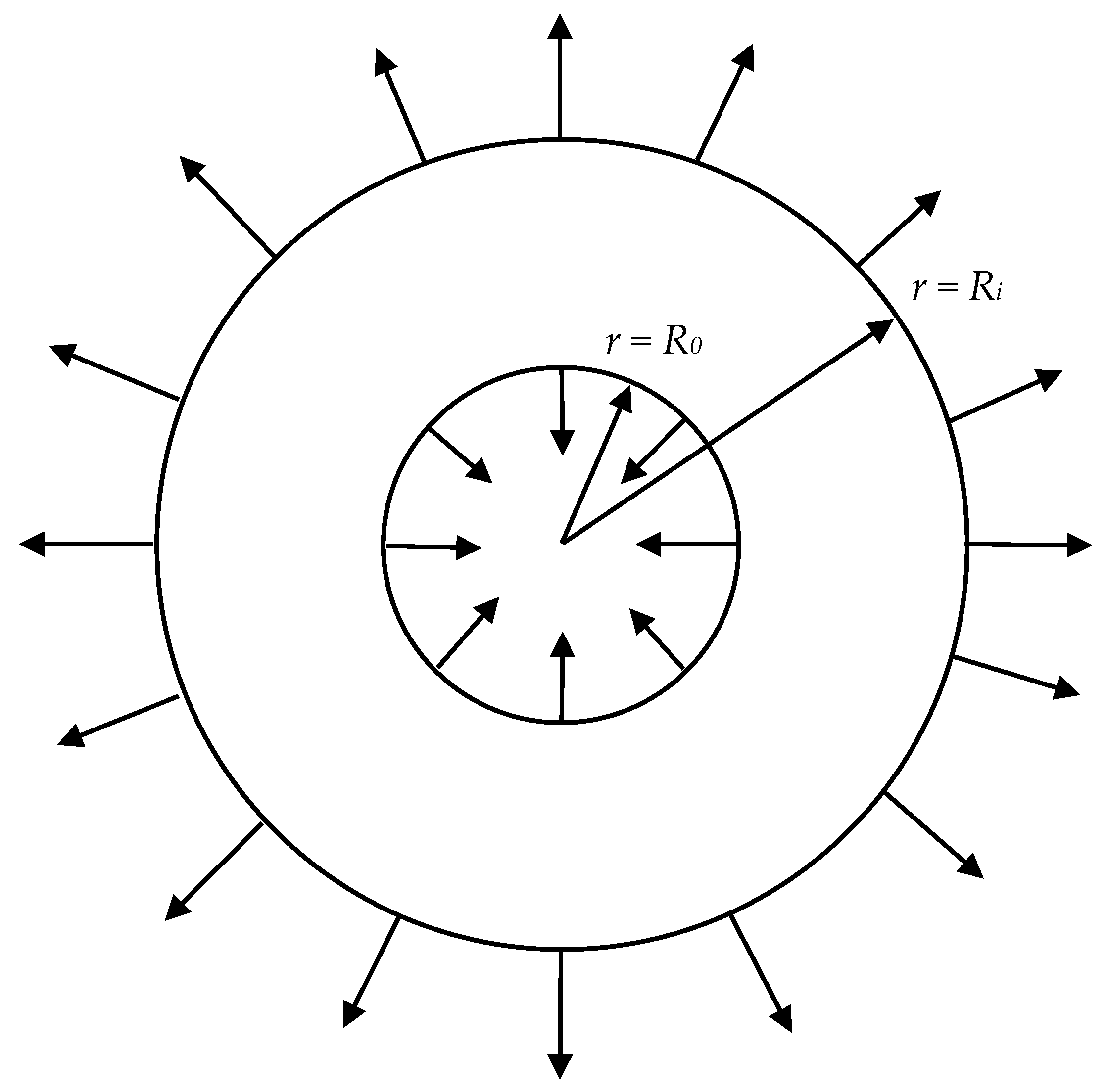
2.1. Statement of the Problem

Considered is an annulus of inner radius R i and outer radius R o . The latter may tend to infinity. Uniform pressure or radial displacement is prescribed at each radius. It is natural to choose a cylindrical coordinate system ( r , θ , z ) whose z -axis coincides with the axis of symmetry of the annulus (Figure 1). The material model is polar orthotropic. The principal axes of anisotropy coincide with the coordinate lines of the cylindrical coordinate system. The solution is independent of θ under the conditions above. The assumption of plane stress and axial symmetry dictates that the only non-zero stresses in the cylindrical coordinate system are σ r and σ θ . Similarly, the only non-zero strains in the cylindrical coordinate system are, ε r , ε θ , and ε z . The strains are infinitesimal and
ε r = ε r e + ε r p ,       ε θ = ε θ e + ε θ p ,   and   ε z = ε z e + ε z p .
Here, the superscript ‘e’ denotes the elastic portion of the strain components, and the superscript ‘p’ denotes their plastic portion. Equation (1) is valid in plastic regions. The whole strain is elastic in elastic regions. The generalized Hooke’s law reads as follows.
ε r e = a r r σ r + a r θ σ θ , ε θ e = a r θ σ r + a θ θ σ θ ,   and   ε z e = a r z σ r + a θ z σ θ .
Here a r r , a r θ , a θ θ , a r z , and a θ z are the components of the compliance tensor. The yield criterion can be represented as
F ( σ r , σ θ ) = 0 .
Here, F is an arbitrary function of its arguments satisfying the conventional restrictions imposed on the yield criteria. It is convenient to rewrite (3) as
σ r = σ 0 f r ( τ )   and   σ θ = σ 0 f θ ( τ ) ,
where σ 0 is a reference stress and τ is a parameter. Taking into account plastic incompressibility, one can represent the plastic flow rule associated with the yield criterion (3) as
ξ r p = λ Φ r ,       ξ θ p = λ Φ θ ,   and   ξ z p = λ ( Φ r + Φ θ ) .
Here, λ is a non-negative multiplier and
Φ r F σ r   and   Φ θ F σ θ .
Using (4), one can express Φ r and Φ θ as functions of τ . Since the material model is rate-independent, the quantities on the left-hand sides of the equations in (5) can be represented as
ξ r p = ε r p p ,       ξ θ p = ε θ p p ,   and   ξ z p = ε z p p .
Here, p is an arbitrary time-like parameter. Accordingly,
ξ r e = ε r e p , ξ θ e = ε θ e p , ξ z e = ε z e p , ξ r = ε r p , ξ θ = ε θ p , ξ z = ε z p .
In particular, it follows from (1) and (2) that
ξ r = ξ r e + ξ r p ,       ξ θ = ξ θ e + ξ θ p ,   and   ξ z = ξ z e + ξ z p .
ξ r e = a r r σ r p + a r θ σ θ p ,   ξ θ e = a r θ σ r p + a θ θ σ θ p , ξ z e = a r z σ r p + a θ z σ θ p .
The only equilibrium equation that is not satisfied identically is
σ r r + σ r σ θ r = 0 .
The strain rate compatibility equation is equivalent to
r ξ θ r = ξ r ξ θ .

2.2. General Elastic Solution

This solution is valid in elastic regions. In this case, the plastic portion of the strain components vanishes. The stress solution is [23]
σ r σ 0 = C 1 ρ m 1 + C 2 ρ m 1   and   σ θ σ 0 = m ( C 1 ρ m 1 C 2 ρ m 1 ) .
Here m = a r r / a θ θ and
ρ = r r 0 .
In addition, r 0 , C 1 , and C 2 are constants. The strain components are determined from (2) and (13) as
ε r = ( A r r + m A r θ ) C 1 ρ m 1 + ( A r r m A r θ ) C 2 ρ m 1 , ε θ = ( A r θ + m A θ θ ) C 1 ρ m 1 + ( A r θ m A θ θ ) C 2 ρ m 1 , ε z = ( A r z + m A θ z ) C 1 ρ m 1 + ( A r z m A θ z ) C 2 ρ m 1 ,
where
A r r = a r r σ 0 , A θ θ = a θ θ σ 0 , A r θ = a r θ σ 0 , A r z = a r z σ 0 , A θ z = a θ z σ 0 .

2.3. General Solution in Plastic Regions

Equation (4) is valid in plastic regions. Substituting this equation into (11) and using (14) gives
μ ( τ ) τ ρ = 1 ρ ,
where
μ ( τ ) = d f r d τ ( f θ f r ) 1 .
The solution of Equation (17) can be written as
ρ = exp [ τ 0 τ μ ( t ) d t ] .
This solution satisfies the boundary condition
ρ = 1   or   r = r 0
where τ = τ 0 . Equations (2) and (4) combine to give
ε r e = A r r f r + A r θ f θ , ε θ e = A r θ f r + A θ θ f θ ,   and   ε z e = A r z f r + A θ z f θ .
Substituting (21) into (8) yields
ξ r e = ( A r r d f r d τ + A r θ d f θ d τ ) τ p , ξ θ e = ( A r θ d f r d τ + A θ θ d f θ d τ ) τ p , ξ z e = ( A r z d f r d τ + A θ z d f θ d τ ) τ p .
Differentiating (19) leads to
μ ( τ ) d τ = d ρ ρ + μ ( τ 0 ) d τ 0 .
Therefore,
τ p = μ ( τ 0 ) μ ( τ ) d τ 0 d p .
Substituting (24) into (22) gives
ξ r e = ( A r r d f r d τ + A r θ d f θ d τ ) μ ( τ 0 ) μ ( τ ) d τ 0 d p , ξ θ e = ( A r θ d f r d τ + A θ θ d f θ d τ ) μ ( τ 0 ) μ ( τ ) d τ 0 d p , ξ z e = ( A r z d f r d τ + A θ z d f θ d τ ) μ ( τ 0 ) μ ( τ ) d τ 0 d p .
By eliminating λ between the equations in (5), one obtains
ξ r p = ξ θ p Φ r Φ θ   and   ξ z p = ξ θ p ( 1 + Φ r Φ θ ) .
Equations (9), (25), and (26) combine to give
ξ r = ( A r r d f r d τ + A r θ d f θ d τ ) μ ( τ 0 ) μ ( τ ) d τ 0 d p + ξ θ p Φ r Φ θ , ξ θ = ( A r θ d f r d τ + A θ θ d f θ d τ ) μ ( τ 0 ) μ ( τ ) d τ 0 d p + ξ θ p , ξ z = ( A r z d f r d τ + A θ z d f θ d τ ) μ ( τ 0 ) μ ( τ ) d τ 0 d p ξ θ p ( 1 + Φ r Φ θ ) .
Replacing differentiation with respect to ρ with differentiation with respect to τ in (12) using (14) and (17), one arrives at
ξ θ τ = ( ξ r ξ θ ) μ ( τ ) .
Using (27), one can transform the right-hand side of this equation as
ξ θ τ = [ ( A r r A r θ ) d f r d τ + ( A r θ A θ θ ) d f θ d τ ] μ ( τ 0 ) d τ 0 d p + ξ θ p μ ( τ ) ( Φ r Φ θ 1 ) .
The second equation in (27) allows for ξ θ p to be eliminated. Then, Equation (29) becomes
ξ θ τ = χ ( τ ) μ ( τ 0 ) d τ 0 d p + ω ( τ ) ξ θ
where
χ ( τ ) = ( A r r A r θ Φ r Φ θ ) d f r d τ + ( A r θ A θ θ Φ r Φ θ ) d f θ d τ , ω ( τ ) = ( Φ r Φ θ 1 ) μ ( τ ) .
The general solution of Equation (30) is
ξ θ = exp [ τ 0 τ ω ( t ) d t ] [ ξ 0 + μ ( τ 0 ) d τ 0 d p τ 0 τ χ ( γ ) exp [ τ 0 γ ω ( t ) d t ] d γ ] .
Here, ξ 0 is a function of p. Its physical sense is that
ξ θ = ξ 0
where τ = τ 0 . Using solution (32), one can find ξ θ p from the second equation in (27). Then, the other two equations in (27) supply ξ r and ξ z . The quantities ξ r p and ξ z p are determined from (9) and (25).
The plastic strains can be found employing (7). These equations are written assuming that their left-hand sides are functions of ρ and p. However, Equation (32) provides ξ θ and, consequently, these left-hand sides as a function of τ and p. If τ is eliminated using (19), then
ε r p = p e p ξ r p ( ρ , t ) d t ,       ε θ p = p e p ξ θ p ( ρ , t ) d t ,   and   ε z p = p e p ξ z p ( ρ , t ) d t .
These integrals are evaluated while ρ is kept a constant. Additionally, p e is the value of p at which plastic yielding begins at a chosen value of ρ . Thus, it depends on ρ .
An alternative way of solving the equations in (7) is to rewrite them, assuming that their left-hand sides depend on τ and p. Employing (24), one obtains
ε r p p + μ ( τ 0 ) μ ( τ ) d τ 0 d p ε r p τ = ξ r p ( τ , p ) , ε θ p p + μ ( τ 0 ) μ ( τ ) d τ 0 d p ε θ p τ = ξ θ p ( τ , p ) , ε z p p + μ ( τ 0 ) μ ( τ ) d τ 0 d p ε z p τ = ξ z p ( τ , p ) .
The characteristics of each of these equations are
d τ d τ 0 = μ ( τ 0 ) μ ( τ ) .
It is seen from this equation that
τ = τ 0
is one of the characteristics. The relations along the characteristics are
ε r p = p e p ξ r p d t ,       ε θ p = p e p ξ θ p d t ,   and   ε z p = p e p ξ z p d t .
It is understood here that τ in the integrands is eliminated using the solution of (36). The total strains are determined from (1), (21) and (34) or (1), (21) and (38).

2.4. Illustrative Example

The solution above is valid for any yield criterion and boundary conditions satisfying the requirements formulated in Section 2.1. The present section illustrates this solution by employing a simple example. It is assumed that r 0 = R i and a = R o / R i . Therefore, 1 ρ a .
The version of the Tsai-Hill yield criterion satisfying the required assumptions is [23]
σ θ 2 σ r σ θ + σ r 2 X 2 Y 2 = X 2 .
Here, X and Y are the tensile yield stresses in the circumferential and radial directions, respectively. Put σ 0 = X . Then, one can choose
f r = 2 sin τ Q   and   f θ = ( sin τ Q + cos τ ) ,
where Q = 4 X 2 Y 2 / Y . It follows from (39) and (40) that
Φ r Φ θ = Q tan τ 1 2 .
Substituting (40) into (18) yields
μ = 2 Q tan τ .
The elastic properties are assumed to be isotropic for a less cumbersome solution. Then,
A r r = A θ θ = k   and   A r θ = A r z = A θ z = ν k ,
where k = σ 0 / E , ν is Poisson’s ratio, and E is Young’s modulus. Solution (13) becomes
σ r σ 0 = C 1 + C 2 ρ 2   and   σ θ σ 0 = C 1 C 2 ρ 2 .
Substituting (41), (42), and (43) into (31) yields
χ ( τ ) = k [ 2 Q ( 2 ν cos 2 τ ) + ν ( 3 + Q 2 ) sin 2 τ ] 2 Q ( Q cos τ + sin τ ) , ω ( τ ) = 2 cos τ Q cos τ + sin τ .
The subsequent solution essentially depends on the boundary conditions. Assume that
σ r = σ 0 s 0
where ρ = 1 and
σ r = σ 0 s
where ρ = a . Substituting (46) and (47) into (44) gives
C 1 = s 0 s a 2 a 2 1   and   C 2 = ( s s 0 ) a 2 a 2 1 .
Eliminating C 1 and C 2 in (44) using (48) supplies the stress solution in a purely elastic disk in the form
σ r σ 0 = s 0 s a 2 a 2 1 + ( s s 0 ) a 2 ( a 2 1 ) ρ 2   and   σ θ σ 0 = s 0 s a 2 a 2 1 ( s s 0 ) a 2 ( a 2 1 ) ρ 2 .
This solution is valid if the yield criterion is not violated in the range 1 ρ a . The radius at which plastic yielding initiates is determined from Equation (39) after eliminating the stresses using the stress solution in a purely elastic disk. It results in a cumbersome bi-quadratic equation, which can be solved analytically. The most realistic scenario is that the plastic region starts to propagate from the inner radius. For definiteness, this case is considered below.
Substituting (49) into (39) at ρ = 1 supplies the following relation between s and s 0 corresponding to the initiation of plastic yielding:
s e = ( 1 + 3 a 2 ) s 0 ± ( a 2 1 ) 4 Q 2 s 0 2 4 a 2 .
The subscript “e” means that this value of s corresponds to the initiation of plastic yielding. In what follows, it is assumed that s 0 is kept a constant and s changes such that the plastic region propagates from the inner radius.
Let ρ c be the elastic–plastic radius. Equation (40) is valid in the range 1 ρ ρ c . In particular, the stress solution in the plastic region must satisfy the boundary condition (46). Then,
sin τ 0 = Q s 0 2 .
The value of τ 0 can be found from this equation and the purely elastic solution after choosing the sign in (51). In either case, τ 0 is constant. Therefore,
d τ 0 d p = 0 .
Substituting (42) into (19) and integrating leads to
ρ = exp [ 2 Q ( 1 + Q 2 ) ( τ τ 0 ) ] ( Q cos τ 0 sin τ 0 Q cos τ sin τ ) h ,
where h = 2 / ( 1 + Q 2 ) . Let τ c be the value of τ at the elastic–plastic radius. It follows from (53) that
ρ c = exp [ 2 Q ( 1 + Q 2 ) ( τ c τ 0 ) ] ( Q cos τ 0 sin τ 0 Q cos τ c sin τ c ) h .
The radial and circumferential stresses must be continuous across the elastic–plastic boundary. Then, Equations (40) and (44) combine to give
2 sin τ c Q = C 1 + C 2 ρ c 2   and   sin τ c Q + cos τ c = C 1 + C 2 ρ c 2 .
Solving these equations for C 1 and C 2 yields
C 1 = ( 3 sin τ c + Q cos τ c ) 2 Q   and   C 2 = ρ c 2 ( Q cos τ c sin τ c ) 2 Q .
Using (44) and (56), one can represent the stress solution in the elastic region as
σ r σ 0 = ( 3 sin τ c + Q cos τ c ) 2 Q + ρ c 2 ( Q cos τ c sin τ c ) 2 Q ρ 2 , σ θ σ 0 = ( 3 sin τ c + Q cos τ c ) 2 Q ρ c 2 ( Q cos τ c sin τ c ) 2 Q ρ 2 .
This solution must satisfy the boundary condition (47). Hence,
a 2 ( 3 sin τ c + Q cos τ c ) ρ c 2 ( Q cos τ c sin τ c ) = 2 Q a 2 s .
It is seen from (54) and (58) that it is convenient to put p τ c . Then, these equations supply the dependencies of ρ c and s on p in analytic form. Equations (40), (53), and (57) allow for the radial and circumferential stresses to be calculated at any values of ρ and p. This solution is valid if ρ c a . Using (54), one can derive the equation for the value of p corresponding to ρ c = a and denoted as p a :
a = exp [ 2 Q ( 1 + Q 2 ) ( p a τ 0 ) ] ( Q cos τ 0 sin τ 0 Q cos p a sin p a ) h .
It remains to find the strain solution. Equations (32) and (52) combine to give
ξ θ = ξ 0 exp [ τ 0 τ ω ( t ) d t ] .
By eliminating here ω using (45) and integrating, one obtains
ξ θ = ξ 0 exp [ 2 Q ( 1 + Q 2 ) ( τ 0 τ ) ] ( Q cos τ 0 + sin τ 0 Q cos τ + sin τ ) h .
It follows from this equation that
ξ θ = ξ 0 exp [ 2 Q ( 1 + Q 2 ) ( τ 0 p ) ] ( Q cos τ 0 + sin τ 0 Q cos p + sin p ) h
on the plastic side of the elastic–plastic boundary. The circumferential strain in the elastic region is determined from (15), (43) and (56) as
ε θ k = ( 1 ν ) ( 3 sin p + Q cos p ) 2 Q ρ c 2 ( Q cos p sin p ) ( 1 + ν ) 2 Q ρ 2 .
Differentiating with respect to p gives
ξ θ k = ( 1 ν ) ( 3 cos p Q sin p ) 2 Q + ρ c 2 ( Q sin p + cos p ) ( 1 + ν ) 2 Q ρ 2 ( Q cos p sin p ) ( 1 + ν ) 2 Q ρ 2 d ( ρ c 2 ) d p .
The derivative d ( ρ c 2 ) / d p is determined from (54) as
d ( ρ c 2 ) d p = 4 cos p ( Q cos p sin p ) ( Q cos τ 0 sin τ 0 Q cos p sin p ) 2 h exp [ 4 Q ( p τ 0 ) 1 + Q 2 ] .
Substituting (65) into (64) and putting ρ = ρ c gives
ξ θ k = Q sin p 3 cos p Q
on the elastic side of the elastic–plastic boundary. Since ξ θ must be continuous, it follows from (62) and (66) that
ξ 0 = k ( Q sin p 3 cos p ) Q ( Q cos p + sin p Q cos τ 0 + sin τ 0 ) h exp [ 2 Q ( 1 + Q 2 ) ( p τ 0 ) ] .
Substituting (41) and (52) into (27) yields
ξ r = ξ r p = ξ θ p ( Q tan τ 1 ) 2 , ξ θ = ξ θ p , ξ z = ξ z p = ξ θ p ( Q tan τ + 1 ) 2 .
Eliminating here ξ θ using (61), one obtains
ξ r p = ξ 0 exp [ 2 Q ( 1 + Q 2 ) ( τ 0 τ ) ] ( Q cos τ 0 + sin τ 0 Q cos τ + sin τ ) h ( Q tan τ 1 ) 2 , ξ θ p = ξ 0 exp [ 2 Q ( 1 + Q 2 ) ( τ 0 τ ) ] ( Q cos τ 0 + sin τ 0 Q cos τ + sin τ ) h , ξ z p = ξ 0 exp [ 2 Q ( 1 + Q 2 ) ( τ 0 τ ) ] ( Q cos τ 0 + sin τ 0 Q cos τ + sin τ ) h ( Q tan τ + 1 ) 2 .
In the case under consideration, τ is independent of p . Therefore, substituting (69) into (38) yields
ε r p = exp [ 2 Q ( 1 + Q 2 ) ( τ 0 τ ) ] ( Q cos τ 0 + sin τ 0 Q cos τ + sin τ ) h ( Q tan τ 1 ) 2 τ p ξ 0 d t , ε θ p = exp [ 2 Q ( 1 + Q 2 ) ( τ 0 τ ) ] ( Q cos τ 0 + sin τ 0 Q cos τ + sin τ ) h τ p ξ 0 d t , ε z p = exp [ 2 Q ( 1 + Q 2 ) ( τ 0 τ ) ] ( Q cos τ 0 + sin τ 0 Q cos τ + sin τ ) h ( Q tan τ + 1 ) 2 τ p ξ 0 d t .
Here, p τ . The integral in the equations in (70) should be evaluated numerically using (67).

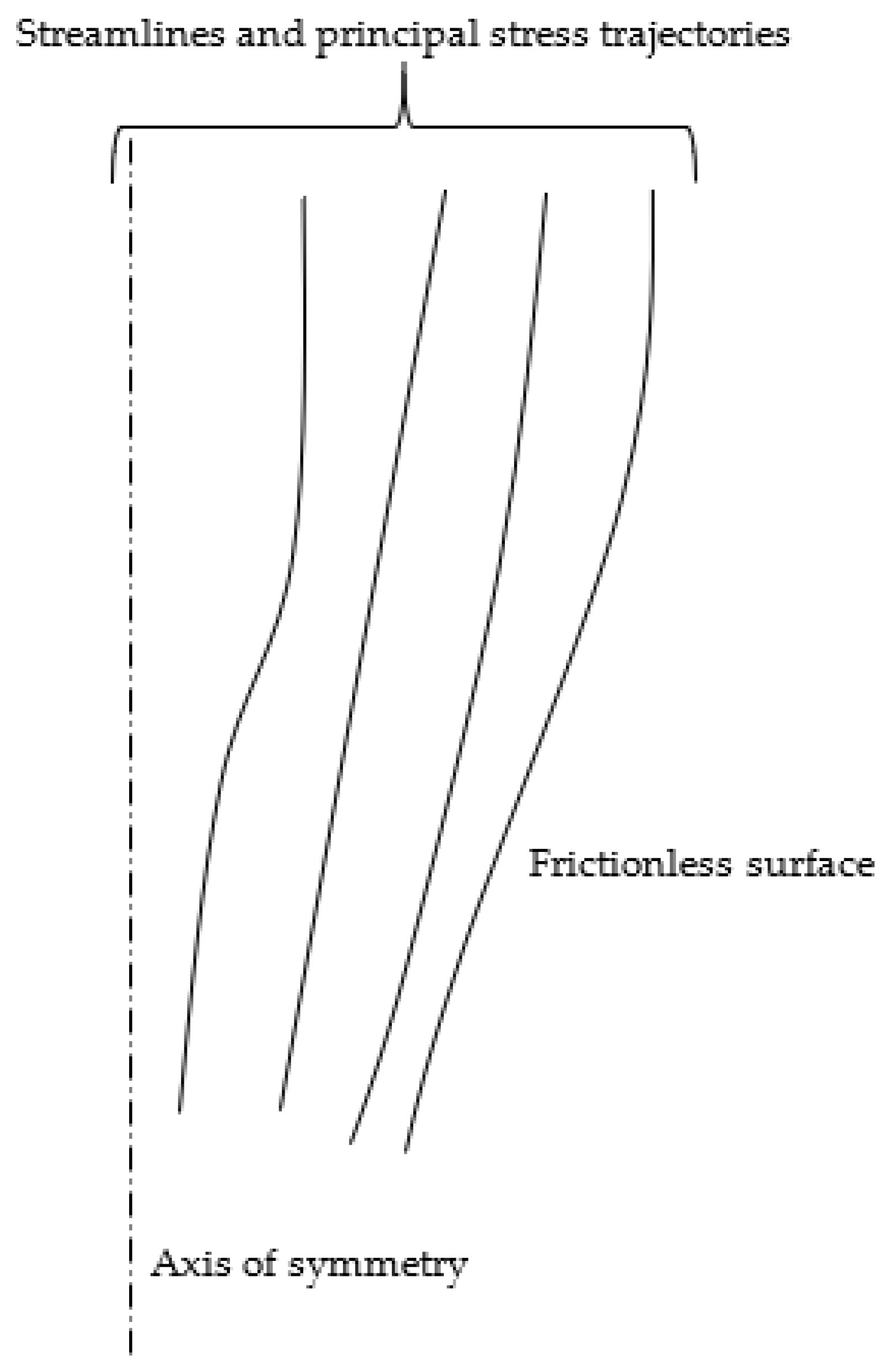
3. Axisymmetric Steady Ideal Flows

In the case of stationary bulk ideal flows, the streamlines coincide with principal stress trajectories. This condition implies that the contact surface between the deformable material and tool is frictionless (Figure 2). Proof of the existence of ideal flow requires showing that the condition above is compatible with a particular material model. The derivation in this section is based on the following main assumptions: (i) rigid plasticity, (ii) yield criterion [32], and (iii) the associated flow rule.

3.1. Constitutive Equations

Considered is an orthotropic rigid plastic material. A generalization of Tresca’s yield criterion on such materials has been proposed in [32]. The key assumption is that the principal axes of stress coincide with the principal axes of anisotropy at all points when the material is plastically deformed. Another assumption, typical for many metallic materials, is that hydrostatic pressure does not affect the plastic flow. Under these assumptions, the yield surface in a three-dimensional space where the principal stresses are taken as Cartesian coordinates is generated by the lines parallel to the line passing through the origin with direction cosines ( 1 / 3 , 1 / 3 , 1 / 3 ) . The circumferential stress σ θ is one of the principal stresses under axial symmetry. The other principal stresses are denoted as σ 1 and σ 2 . The π -plane is defined by the equation σ 1 + σ 2 + σ θ = 0 . The cross-section of the yield surface proposed in [32] with this plane is shown in Figure 3. Several flow regimes depend on the yield locus’s particular side or vertex. It is possible to assume with no loss of generality that
σ 2 > σ 1 .
Then, the regimes important for the ideal flow theory correspond to points A and C (Figure 3). These regimes will be considered below.
The equations of faces AB, AC, and CD are
σ 1 ( σ 20 σ 30 ) + σ 2 σ 30 σ θ σ 20 = σ 20 σ 30 , σ 2 σ 10 σ 1 σ 20 + σ θ ( σ 20 σ 10 ) = σ 20 σ 10 , σ 1 σ 30 + σ 2 ( σ 30 σ 10 ) + σ θ σ 10 = σ 30 σ 10 ,
respectively. Here, σ 10 , σ 20 , and σ 30 are the yield stresses in the principal directions of anisotropy. The equations in (72) reduce to the Tresca yield criterion if σ 10 = σ 20 = σ 30 . Let ξ 1 , ξ 2 , and ξ θ be the principal strain rates. The latter is also the circumferential strain rate. The plastic flow rule associated with point A is
ξ 1 = λ 1 ( σ 20 σ 30 ) λ 2 σ 20 , ξ 2 = λ 1 σ 30 + λ 2 σ 10 , ξ θ = λ 1 σ 20 + λ 2 ( σ 20 σ 10 ) .
The plastic flow rule associated with point C is
ξ 1 = λ 1 σ 20 λ 2 σ 30 , ξ 2 = λ 1 σ 10 + λ 2 ( σ 30 σ 10 ) , ξ θ = λ 1 ( σ 20 σ 10 ) + λ 2 σ 10 .
In the equations in (73) and (74),
λ 1 0   and   λ 2 0
It is seen from (73) and (74) that
ξ 1 + ξ 2 + ξ θ = 0 ,
which is the incompressibility equation. It follows from (72) that the edge of the yield surface corresponding to point A can be represented as
σ 1 = σ θ = σ 2 σ 20 .
The edge corresponding to point C can be represented as
σ 2 = σ θ = σ 1 σ 10 .

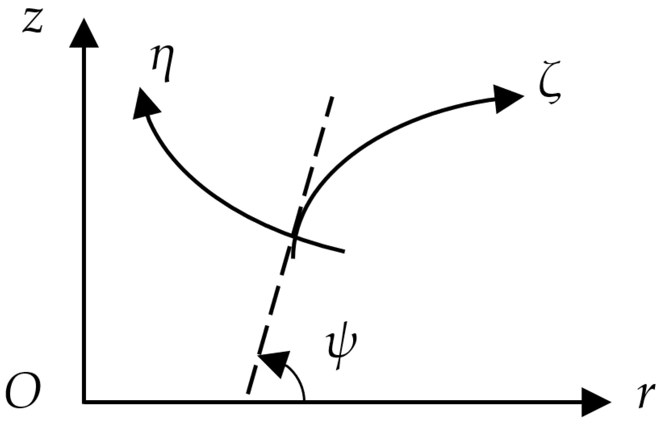
3.2. Geometric Properties of the Principal Lines Coordinate System

A cylindrical coordinate system ( r , θ , z ) whose z -axis coincides with the axis of symmetry is introduced. Under axial symmetry, it is always possible to choose an orthogonal coordinate system ( ζ , θ , η ) whose coordinate lines coincide with the trajectories of the principal stresses. This coordinate system is named the principal lines coordinate system. The scale factors of the principal lines coordinate system are h ζ , r, and h η . In what follows, it is assumed that the trajectories of the stress σ 1 are ζ -lines, and the trajectories of the stress σ 2 are η -lines. By definition, the shear stresses vanish in the principal lines coordinate system. Then, the stress equilibrium equations are [34]
( r h η σ 1 ) ζ σ θ h η r ζ r σ 2 h η ζ = 0   and   ( r h ζ σ 2 ) η r σ 1 h ζ η σ θ h ζ r η = 0 .
Consider the regime of flow corresponding to point A (Figure 3). This edge is the intersection of faces AC and AB. The first two equations in (72) result in
σ 1 = σ θ .
Then, the first equation in (72) transforms to
σ 2 = σ 1 + σ 20 .
Substituting (80) and (81) into (79) yields
σ 1 ζ = σ 20 h η h η ζ   and   r h ζ σ 1 η = σ 20 ( r h ζ ) η .
Each of these equations can be immediately integrated to give
σ 1 = σ 20 ln ( h η H η ( η ) )   and   σ 1 = σ 20 ln ( r h ζ H ζ ( ζ ) ) .
Here, H η ( η ) is an arbitrary function of η , and H ζ ( ζ ) is an arbitrary function of ζ . However, it is evident from (83) that different choices of these functions merely change the scale of the η - and ζ -lines, respectively. Therefore, it is always possible to put H η ( η ) = H ζ ( ζ ) = 1 . Then, Equation (84) becomes
σ 1 = σ 20 ln h η   and   σ 1 = σ 20 ln ( r h ζ ) .
Eliminating σ 1 between the equations in (84) gives
r h ζ h η = 1 .
The flow regime corresponding to point C can be treated similarly.

3.3. Existence of Ideal Flows

Let u ζ and u η be the velocity components referred to the ( ζ , η ) -coordinate system. The strain rate components referred to this coordinate system are [34]
ξ ζ ζ = 1 h ζ u ζ ζ + u η h ζ h η h ζ η , ξ η η = 1 h η u η η + u ζ h ζ h η h η ζ , 2 ξ ζ η = 1 h ζ u η ζ + 1 h η u ζ η u ζ h ζ h η h ζ η u η h ζ h η h η ζ .
The ideal flow condition at point A (Figure 3) is that the η -lines are streamlines. Therefore, u ζ = 0 everywhere and Equation (87) becomes
ξ ζ ζ = u η h ζ h η h ζ η , ξ η η = 1 h η u η η , 2 ξ ζ η = 1 h ζ u η ζ u η h ζ h η h η ζ .
The circumferential strain rate is
ξ θ θ = u r r .
Here, u r is the radial velocity. It follows from (87) and (88) that Equation (76) is equivalent to
u η h ζ h η h ζ η + 1 h η u η η + u r r = 0 .
Let ψ be the inclination of the ζ -lines to the r -axis measured from the axis anticlockwise (Figure 4). Then,
r ζ = h ζ cos ψ , r η = h η sin ψ ,   and   u r = u η sin ψ .
Using (90), one can rewrite Equation (89) as
u η h ζ h ζ η + u η η + u η r r η = 0 .
This equation can be immediately integrated to give
u η = U r h ζ .
Using (85), one can transform this equation to
u η = U h η .
Substituting (93) into the third equation in (87) shows that ξ ζ η = 0 if U is constant.
The velocity component u η from (93) satisfies the incompressibility equation and the ideal flow conditions. The other equations of the plastic flow rule reduce to checking the inequalities in (75). Therefore, the existence of ideal flow solutions has been proven.
Finding an ideal flow solution is reduced to finding an orthogonal coordinate system in a meridional plane satisfying (85). However, the latter coincides with the corresponding equation for Tresca’s yield criterion [35]. Therefore, the principal line coordinate systems that can be found from the available solutions for Tresca’s yield criterion apply to the material model under consideration.

4. Miscellaneous Topics

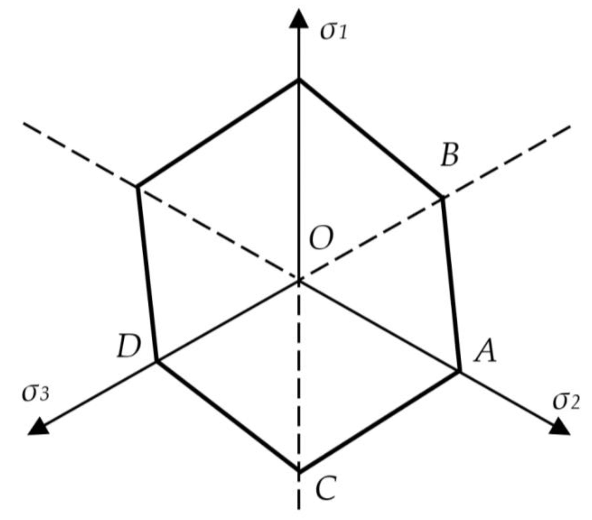
4.1. Yield Criterion

The yield criterion is one of the basic constituents of the classical models in plasticity. The topics reviewed in the two previous sections require special cases of the totality of possible yield criteria. A systematic overview of anisotropic yield criteria has been provided in [33]. It is worthy of note that the assumption of normal anisotropy is often used under plane-stress conditions ([36,37,38,39] among many others). This simplification can considerably affect theoretical stress and strain fields that would result from solutions without it [40].

4.2. Limit Load

The limit load is an important parameter in engineering. For instance, it is an essential input parameter of flaw assessment procedures [41]. The application of the upper-bound theorem does not differ from that for isotropic materials. In particular, any kinematically admissible velocity field for isotropic models is a kinematically admissible velocity field for anisotropic models. However, the limit load is significantly affected by plastic anisotropy ([42,43] among many others). Generalizing isotropic lower bound solutions based on piece-wise constant stress fields on anisotropic models is also straightforward. Examples of such isotropic solutions have been provided, for example, in [44,45].

4.3. Singular Solutions

The plane strain equations of rigid–plastic anisotropic solids are hyperbolic [46,47]. It has been shown in [48] that some components of the strain-rate tensor approach infinity near envelopes of characteristics. The exact asymptotic representation of these components depends on the yield criterion. Knowing such representations is important for developing numerical codes. In particular, traditional finite element methods are not capable of solving the boundary value problems involving the singularity above, even for a simpler model [49].

5. Conclusions

Plastic anisotropy is a common property of most metallic materials. The present paper has presented an overview of two selected issues of the mathematical theory of the plasticity of such materials. This overview does not pretend to be comprehensive. Section 2 and Section 3 discuss the issues not included in available review articles and monographs. The former deals with a general elastic–plastic solution for a particular geometry and particular orientation of the principal axes of anisotropy. The latter extends the ideal flow theory to anisotropic materials under axial symmetry. Section 4 collects three short remarks on anisotropic yield criteria, limit load solutions, and singular solutions.
The applied aspects of two main issues considered are that polar orthotropic disks are widely used in the industry, and the ideal flow theory is a tool for the metal forming design.

Author Contributions

Conceptualization, S.A.; formal analysis, M.R.; writing—review and editing, S.A. All authors have read and agreed to the published version of the manuscript.

Funding

This research received no external funding.

Institutional Review Board Statement

Not applicable.

Informed Consent Statement

Not applicable.

Data Availability Statement

Not applicable.

Acknowledgments

This paper has been supported by the RUDN University Strategic Academic Leadership Program.

Conflicts of Interest

The authors declare no conflict of interest.

References

  1. Varga, O.H. Stress-Strain Behaviour of Elastic Materials; Interscience: New York, NY, USA, 1966. [Google Scholar]
  2. Hill, J.M.; Arrigo, D.J. Transformations and equation reductions in finite elasticity I: Plane strain deformations. Math. Mech. Solids 1996, 1, 155–175. [Google Scholar] [CrossRef]
  3. Hill, J.M.; Arrigo, D.J. Transformations and equation reductions in finite elasticity II: Plane stress and axially symmetric deformations. Math. Mech. Solids 1996, 1, 177–192. [Google Scholar] [CrossRef]
  4. Murphy, J.G. Irrotational deformations in finite compressible elasticity. Math. Mech. Solids 1997, 2, 491–502. [Google Scholar] [CrossRef]
  5. Israilov, M.S. Reduction of boundary value problems of dynamic elasticity to scalar problems for wave potentials in curvilinear coordinates. Mech. Solids 2011, 46, 104–108. [Google Scholar] [CrossRef]
  6. Ostrosablin, N.I. The general solution and reduction to diagonal form of a system of equations of linear isotropic elasticity. J. Appl. Ind. Math. 2010, 4, 354–358. [Google Scholar] [CrossRef]
  7. Simmonds, J.G. Reduction of the linear Sanders-Koiter shell equations for nondevelopable midsurfaces to two coupled equations. ASME J. Appl. Mech. 1975, 42, 511–513. [Google Scholar] [CrossRef]
  8. Reissner, E. On reductions of the differential equations for circular cylindrical shells. Ingenieur-Archiv 1972, 41, 291–296. [Google Scholar] [CrossRef]
  9. Zhou, Y.; Huang, K. An effective general solution to the inhomogeneous spatial axisymmetric problem and its applications in functionally graded materials. Acta Mech. 2021, 232, 4199–4215. [Google Scholar] [CrossRef]
  10. Tokovyy, Y.V. Reduction of a three-dimensional elasticity problem for a finite-length solid cylinder to the solution of systems of linear algebraic equations. J. Math. Sci. 2013, 190, 683–696. [Google Scholar] [CrossRef]
  11. Durban, D. An approximate method in plane-stress small strain plasticity. ASME J. Appl. Mech. 1987, 54, 968–970. [Google Scholar] [CrossRef]
  12. Alexandrova, N.; Alexandrov, S. Elastic-plastic stress distribution in a plastically anisotropic rotating disk. Trans. ASME J. Appl. Mech. 2004, 71, 427–429. [Google Scholar] [CrossRef]
  13. Alexandrova, N.; Real, P.M.M.V. Elastic-plastic stress distribution in a plastically anisotropic rotating disk. Thin-Walled Struct. 2006, 44, 897–903. [Google Scholar] [CrossRef]
  14. Peng, X.-L.; Li, X.-F. Elastic analysis of rotating functionally graded polar orthotropic disks. Int. J. Mech. Sci. 2012, 60, 84–91. [Google Scholar] [CrossRef]
  15. Essa, S.; Argeso, H. Elastic analysis of variable profile and polar orthotropic FGM rotating disks for a variation function with three parameters. Acta Mech. 2017, 228, 3877–3899. [Google Scholar] [CrossRef]
  16. Jeong, W.; Alexandrov, S.; Lang, L. Effect of plastic anisotropy on the distribution of residual stresses and strains in rotating annular disks. Symmetry 2018, 10, 420. [Google Scholar] [CrossRef] [Green Version]
  17. Yildirim, V. Numerical/analytical solutions to the elastic response of arbitrarily functionally graded polar orthotropic rotating discs. J. Brazilian Soc. Mech. Sci. Eng. 2018, 40, 320. [Google Scholar] [CrossRef]
  18. Leu, S.-Y.; Hsu, H.-C. Exact solutions for plastic responses of orthotropic strain-hardening rotating hollow cylinders. Int. J. Mech. Sci. 2010, 52, 1579–1587. [Google Scholar] [CrossRef]
  19. Abd-Alla, A.M.; Mahmoud, S.R.; AL-Shehri, N.A. Effect of the rotation on a non-homogeneous infinite cylinder of orthotropic material. Appl. Math. Comp. 2011, 217, 8914–8922. [Google Scholar] [CrossRef]
  20. Lubarda, V.A. On pressurized curvilinearly orthotropic circular disk, cylinder and sphere made of radially nonuniform material. J. Elast. 2012, 109, 103–133. [Google Scholar] [CrossRef]
  21. Croccolo, D.; De Agostinis, M. Analytical solution of stress and strain distributions in press fitted orthotropic cylinders. Int. J. Mech. Sci. 2013, 71, 21–29. [Google Scholar] [CrossRef]
  22. Shahani, A.R.; Torki, H.S. Determination of the thermal stress wave propagation in orthotropic hollow cylinder based on classical theory of thermoelasticity. Cont. Mech. Thermodyn. 2018, 30, 509–527. [Google Scholar] [CrossRef]
  23. Rynkovskaya, M.; Alexandrov, S.; Lang, L. A theory of autofrettage for open-ended, polar orthotropic cylinders. Symmetry 2019, 11, 280. [Google Scholar] [CrossRef] [Green Version]
  24. Lyamina, E. Effect of plastic anisotropy on the collapse of a hollow disk under thermal and mechanical loading. Symmetry 2021, 13, 909. [Google Scholar] [CrossRef]
  25. Chung, K.; Alexandrov, S. Ideal flow in plasticity. Appl. Mech. Rev. 2007, 60, 316–335. [Google Scholar] [CrossRef]
  26. Richmond, O.; Devenpeck, M.L. A die profile for maximum efficiency in strip drawing. In Proceedings of the 4th US National Congress of Applied Mechanics, Berkeley, CA, USA, 18–21 June 1962; Rosenberg, R.M., Ed.; ASME: New York, NY, USA, 1962; Volume 2, pp. 1053–1057. [Google Scholar]
  27. Richmond, O.; Morrison, H.L. Streamlined wire drawing dies of minimum length. J. Mech. Phys. Solids 1967, 15, 195–203. [Google Scholar] [CrossRef]
  28. Hill, R. Ideal forming operations for perfectly plastic solids. J. Mech. Phys. Solids 1967, 15, 223–227. [Google Scholar] [CrossRef]
  29. Richmond, O.; Alexandrov, S. The theory of general and ideal plastic deformations of Tresca solids. Acta Mech. 2002, 158, 33–42. [Google Scholar] [CrossRef]
  30. Alexandrov, S.; Mustafa, Y.; Lyamina, E. Steady planar ideal flow of anisotropic materials. Meccanica 2016, 51, 2235–2241. [Google Scholar] [CrossRef]
  31. Collins, I.F.; Meguid, S.A. On the influence of hardening and anisotropy on the plane-strain compression of thin metal strip. ASME J. Appl. Mech. 1977, 44, 271–278. [Google Scholar] [CrossRef]
  32. Hu, L.W. Modified Tresca’s yield condition and associated flow rules for anisotropic materials and applications. J. Franklin. Inst. 1958, 265, 187–204. [Google Scholar] [CrossRef]
  33. Barlat, F.; Kuwabara, T.; Korkolis, Y.P. Anisotropic plasticity and application to plane stress. In Encyclopedia of Continuum Mechanic; Altenbach, H., Öchsner, A., Eds.; Springer: Berlin/Heidelberg, Germany, 2018. [Google Scholar]
  34. Malvern, L.E. Introduction to the Mechanics of a Continuous Medium; Prentice-Hall: Englewood Cliffs, NJ, USA, 1969. [Google Scholar]
  35. Alexandrov, S.; Lyamina, E.A.; Nguyen-Thoi, T. Geometry of principal stress trajectories for a Tresca material under axial symmetry. J. Phys. Conf. Ser. 2018, 1053, 012048. [Google Scholar] [CrossRef] [Green Version]
  36. Verma, R.K.; Haldar, A. Effect of normal anisotropy on springback. J. Mater. Process. Technol. 2007, 190, 300–304. [Google Scholar] [CrossRef]
  37. Li, D.; Luo, Y.; Peng, Y.; Hu, P. The numerical and analytical study on stretch flanging of V-shaped sheet metal. J. Mater. Process. Technol. 2007, 189, 262–267. [Google Scholar] [CrossRef]
  38. Paul, S.K. Non-linear correlation between uniaxial tensile properties and shear-edge hole expansion ratio. J. Mater. Eng. Perform. 2014, 23, 3610–3619. [Google Scholar] [CrossRef]
  39. Kim, J.H.; Kwon, Y.J.; Lee, T.; Lee, K.-A.; Kim, H.S.; Lee, C.S. Prediction of hole expansion ratio for various steel sheets based on uniaxial tensile properties. Met. Mater. Int. 2018, 24, 187–194. [Google Scholar] [CrossRef]
  40. Erisov, Y.; Surudin, S.; Alexandrov, S.; Lang, L. Influence of the replacement of the actual plastic orthotropy with various approximations of normal anisotropy on residual stresses and strains in a thin disk subjected to external pressure. Symmetry 2020, 12, 1834. [Google Scholar] [CrossRef]
  41. Zerbst, U.; Madia, M. Analytical flaw assessment. Eng. Fract. Mech. 2018, 187, 316–367. [Google Scholar] [CrossRef]
  42. Alexandrov, S.; Tzou, G.-Y.; Hsia, S.-Y. Effect of plastic anisotropy on the limit load of highly undermatched welded specimens in bending. Eng. Fract. Mech. 2008, 75, 3131–3140. [Google Scholar] [CrossRef]
  43. Alexandrov, S.; Lyamina, E.; Pirumov, A.; Nguyen, D.K. A limit load solution for anisotropic welded cracked plates in pure bending. Symmetry 2020, 12, 1764. [Google Scholar] [CrossRef]
  44. Picon, R.; Canas, J. On strength criteria of fillet welds. Int. J. Mech. Sci. 2009, 51, 609–618. [Google Scholar] [CrossRef]
  45. Hasegawa, K.; Dvorak, D.; Mares, V.; Strnadel, B.; Li, Y. Fully plastic failure stresses and allowable crack sizes for circumferentially surface-cracked pipes subjected to tensile loading. ASME J. Press. Ves. Technol. 2022, 144, 011303. [Google Scholar] [CrossRef]
  46. Rice, J.R. Plane strain slip line theory for anisotropic rigid/plastic materials. J. Mech. Phys. Solids 1973, 21, 63–74. [Google Scholar] [CrossRef]
  47. Hill, R. Basic stress analysis of hyperbolic regimes in plastic media. Math. Proceed. Camb. Philos. Soc. 1980, 88, 359–369. [Google Scholar] [CrossRef]
  48. Alexandrov, S.; Jeng, Y.R. Singular rigid/plastic solutions in anisotropic plasticity under plane strain conditions. Continuum. Mech. Thermodyn. 2013, 25, 685–689. [Google Scholar] [CrossRef]
  49. Facchinetti, M.; Miszuris, W. Analysis of the maximum friction condition for green body forming in an ANSYS environment. J. Europ. Ceramic Soc. 2016, 36, 2295–2302. [Google Scholar] [CrossRef]
Figure 1. Illustration of the boundary value problem.
Symmetry 14 02172 g001
Figure 2. Illustration of the ideal flow condition.
Symmetry 14 02172 g002
Figure 3. Yield locus corresponding to the criterion proposed in [32].
Symmetry 14 02172 g003
Figure 4. Cylindrical and principal lines coordinate systems.
Symmetry 14 02172 g004
Publisher’s Note: MDPI stays neutral with regard to jurisdictional claims in published maps and institutional affiliations.

