Article

Modeling of Cross Work Hardening and Apparent Normality Loss after Biaxial–Shear Loading Path Change

1
Arts et Metiers Institute of Technology, Université de Lorraine, LCFC, HESAM Université, F-57070 Metz, France
2
State Key Lab of Solidification Processing, School of Materials Science and Engineering, Northwestern Polytechnical University, Xi’an 710072, China
*
Author to whom correspondence should be addressed.
Symmetry 2022, 14(1), 142; https://doi.org/10.3390/sym14010142
Submission received: 6 December 2021 / Revised: 26 December 2021 / Accepted: 8 January 2022 / Published: 12 January 2022

Abstract

:
The specific loading-path change during sheet metal forming may lead to some abnormal deformation phenomena. Two-stage orthogonal loading paths without elastic unloading have revealed a phenomenon of apparent loss of normality, further modeled in the literature by non-normality theories. In this paper, a particular orthogonal strain-path change is investigated using the Teodosiu–Hu hardening rule within an associated plasticity framework. The results indicate that cross work-hardening has a significant contribution to the apparent loss of normality and subsequent asymmetric yield surface evolution. Detailed contributions of the model’s ingredients and features are clarified. The developed material model is intended for sheet metal forming simulation applications.

1. Introduction

With an increasing demand for more complicated structure components and more complex shapes of sheet metal parts, the multi-stage forming method needs to be applied. During the multi-stage forming processes, the metal sheet usually undergoes multi-step deformation histories, which raises challenges in describing the material behavior. Indeed, the effect of strain path changes, which occurs during forming processes, is needed to be considered in the constitutive modeling.
During the past decades, many studies have been devoted to revealing the material behavior under complex loading path changes. The different loading path changes during metal deformation usually affect the evolution of plastic anisotropy and work hardening, which should be considered in constitutive modeling. Li et al. [1] explored strain-path change effect on the variation in plastic anisotropy of IF steel via a biaxial–uniaxial tension test, which states the role of crystallographic texture and microstructure evolution during material deformation. Furthermore, they used a meso-scaled constitutive model to predict earing behavior, which emphasizes the importance of the consideration of plastic anisotropy causing the loading path change. Hu [2] also studied work hardening-induced anisotropy of rolled sheet metals, not only using anisotropic coefficients, but also taking into account stress-components and strain-ratios. Mánik et al. [3] applied a successive uniaxial tension tests in rolling followed by transverse direction to investigate the evolutions of transient stress, work-hardening, and Lankford values of aluminum under a cross-loading path change. Based on the experimental findings, they proposed a continuum plasticity model that used a “delayed pointer” tensor to represent the microstructural anisotropy evolution under a cross-loading path change. In addition, the material model could be further enriched to describe mechanical property changes caused by complex material processing methods such as aging and heat treatment, etc., as discussed in [4].
Concerning the effect of strain-path change on work hardening, many studies have been reported as well. Haddadi et al. [5] developed a microstructural-based hardening model, which was applied to describe the anisotropic hardening under tension and shear loading paths change. The early re-yielding behavior, transient hardening, and cross hardening were found in Bauschinger shear and orthogonal tension-shear loading paths, which were correctly described by the models [6]. Wang et al. [7] also simulated a tension–shear test using proposed constitutive model that considers anisotropic hardening effects under an orthogonal strain-path change. Thuillier and Manach [8] compared the strain hardening behaviors of steel sheets by using tensile and shear–strain paths to clarify the effect of loading path. Vincze et al. [9] performed material tests under two-step uniaxial tension along rolling and transverse directions successively. They found that the influences of the pre-strain amounts, severity of loading path change, and subsequent work-hardening can be captured by the model proposed in [10]. Recently, a new constitutive model for describing transient hardening phenomenon is proposed in [11], where the orthogonal strain-path changes and Bauschinger effects are modeled by yield surface distortion and kinematic hardening, respectively.
Because anisotropic plasticity and strain hardening behavior of materials are dependent on loading histories, the evolution of yield surface needs to be accurately described under different strain path changes. Kuroda and Tvergaard [12] used three different methods: uniaxial/biaxial loading, biaxial loading–unloading–reloading, and biaxial–shear loading path changes without unloading, to determine the yield surface evolution of aluminum and steel. Compared with the yield surface determined by using the uniaxial/biaxial loading and biaxial loading–unloading–reloading methods, they found that a vertex appears at the biaxial loading, followed by shear loading path change point, as well as non-normality flow behavior in the second loading path. Khan et al. [13] systemically studied the yield surface evolution under different loading–unloading paths at finite plastic strain6061 aluminum alloy. They found that the J2 yield criterion can well describe the translated and distorted of yield surface evolution. Furthermore, the non-symmetric nose-like shape of yield loci was observed in orthogonal tension–torsion loading path. The similar experimental results were observed for 1100 aluminum alloy in [14]. However, compared with the cross-softening effect on the yield surface evolution for Al6061, the Al1100 had a cross hardening at finite deformation under the tension–torsion loading path [15]. Recently, Iftikhar and Khan [16] investigated the subsequent yield surface evolution subjected proportional/non-proportional loading paths with finite plastic deformation. The results show that the asymmetric yield surface evolution under proportional loading–unloading paths. In addition, Hu et al. [17] first performed three pre-strain loadings under tension, torsion, and combined tension–torsion for steel, and the von Mises type initial yield surface is determined. Later, they found that the size of yield surface was shrinking due to the cross softening. Furthermore, the shape of the yield surface no longer obeyed the symmetry of von Mises’ circle. Lu et al. [18] found that the pre-cyclic loading direction and pre-strain levels have a strong effect on the evolution of yield surface. Furthermore, the obvious asymmetric corner effects lead the subsequent yield surface changes from the von Mises symmetry circle to a distorted asymmetry ellipse. The above discussed experimental investigations indicate that the specific yield surface evolution is strongly dependent on the material load history.
A lot of contributions have been made by researchers to predict the vertex effect and non-normality on the yield surface evolution. Gotoh [19] formulated a classical and the simplest constitutive model to describe the vertex effect concerning rigid-/elastic-plastic materials [20]. Hughes and Shakib [21] proposed a simplified von Mises plasticity, which could represent the corner plastic flow theory. Simo [22] also used a modified J2 theory to interpret the non-normality flow effect caused by a sharp corner at the loading point changes on the yield loci. Kuroda and Tvergaard [23] used a crystal plasticity model to represent non-associated observations. Furthermore, they developed a plasticity model that incorporated the effect of the plastic spin via a vertex flow rule on flat yield loci in [24]. Based on their previous studies, Kuroda [25] proposed a size-independent corner-like plasticity model, which considers the plastic strain gradients effect on the loss of normality. Stoughton [26] applied a non-normality rule with two independent functions of plastic potential and stress yield to describe the flow behavior of steel and aluminum. Cvitanić et al. [27] implemented non- normality constitutive framework into finite element codes. Safaei et al. [28] systemically numerical integration methods for classical constitutive models based on non-normality rule. Based on their work, more advanced hardening models have been investigated as well [29,30,31]. Recently, Chen et al. [11] accurately predicted the earring for the 6014 aluminum deep-drawn part by using constitutive models consisting of different anisotropic yield criteria and non-normality flow rule.
Based on the experimental investigation in [32], the vertex at loading path-change point, and apparent loss of normality and symmetry in the second loading path, are explored. An advanced constitutive model was employed to predict such plastic behaviors after strain-path changes. The effects of rate sensitivity, isotropic/kinematic hardening, and degradation of elastic modulus have been taken into account to explain experimental observations in previous work [33] with a Chaboche-like model. However, in this type of strain-path change biaxial-to-shear, the first loading path, and subsequent loading path, are orthogonal. As a results, this typical loading path introduces cross hardening, which plays a role in subsequent yield locus evolution and normality loss. Recently, the role of the cross-hardening effect has been discussed within the framework of crystal plasticity [34,35]. However, the ingredient of cross hardening that has a significant contribution to the apparent violation of the normality condition and subsequent yield surface evolution need to be investigated at the classical plasticity.
In this paper, the orthogonal biaxial followed by shear loading path change is studied using a modified microstructural-based Teodosiu–Hu hardening model within a framework of associated plasticity. Detailed contributions of the model’s ingredients and features were clarified.

2. Constitutive Modeling

2.1. Elasto-Visco-Plastic Constitutive Framework

In this section, an elasto-visco-plastic (EVP) model is formulated within a convenient rotation frame where the rate form of deformation and internal state variables are used. This approach has an advantage in formulating the applied material models with an identical form as in small strains, which can be accurately adopted in the finite element implementation. When an ideal tension–compression symmetric material deforms into plastic regime, its work hardening behavior usually evolves in a complex way that may break the original symmetry of the yield locus. Generally, the shape and the center of the yield locus can change and translate according to an arbitrary hardening model. Due to this work concentrates on cross hardening modeling, the von Mises yield locus is chosen in the paper.
According to basic theory of metal forming, the total strain rate ε ˙ is made up of the elastic strain rate ε ˙ e and the visco-plastic strain rate ε ˙ v p . The hypo-elastic law can be given by
σ ˙ = C : ε ˙ e = C : ε ˙ ε ˙ v p ,
where σ ˙ is the stress rate and C = 2 G I 4 s + K I I is the fourth-order tensor in the case of isotropic linear elasticity. The scalars G and K can be computed with using Young’s modulus E and Poisson’s ratio v . The ingredients of second order unit tensor I are the Kronecker deltas in which I k l = δ k l . While I 4 s is the fourth-order symmetric deviatoric unit tensor and its components are I 4 i j k l s = 1 / 2 δ i k δ j l + δ i l δ j k 1 / 3 δ i j δ k l . The visco-plastic strain rate tensor ε ˙ v p is formed
ε ˙ v p = ε ¯ ˙ v p · σ ¯ σ = ε ¯ ˙ v p · V ,
where V is the plastic flow direction governed by the associated flow rule, σ ¯ σ X is the von Mises stress and σ indicates the deviatoric part of the stress tensor. The second order tensor X represents the kinematic hardening. The equivalent visco-plastic strain rate ε ¯ ˙ v p is assumed to obey the equation
ε ¯ ˙ v p = ε ˙ # · sinh σ # / k # ,
where k # and ε ˙ # are model parameters, which respond to the visco-plastic effect of material. The “overstress” σ # represents the increase in the stress intensity due to the visco effect-plastic behavior, which is expressed as:
σ ¯ σ X Y σ # 0 ,
where Y describes the size of the yield locus. The equality sign corresponds to elasto-viscoplastic loading, while the inequality sign denotes elastic loading.

2.2. Modified Teodosiu–Hu Hardening Model

With the consideration of the texture evolution under two-step loading at small deformation, a Teodosiu–Hu hardening (THH) model was proposed by Teodosiu and Hu [36]. The focused THH model also has an ability to describe not only the Bauschinger effect but also path dependent hardening behavior after strain-path change.
In THH model, the planar persistent dislocation structures (PPDS) describe the microstructure evolution that contributes to the strain hardening of the material. This model includes four internal state variables:   R , X , S ,   P . The variable R is a scalar, while X and P are second-order tensors and S is fourth order tensor.
The size of yield locus Y is calculated by a function of R and S in Equation (5):
Y = Y 0 + R + f S ,
where Y 0 is the initial yield stress. R represents the contribution of the isotropic hardening, which uses Swift type
R ˙ = H R · ε ¯ ˙ v p = n · K 1 / n K ε 0 n + R n 1 / n · ε ¯ ˙ v p ,
where K , ε 0 , and n are the parameters of Swift law. In Equation (5), f S captures the effect of PPDS on loading path-dependent hardening where f is a material parameter and S is in charge of describing the directional strength of the PPDS.
In this work, a Ziegler type kinematic hardening rule is formulated by the backstress variable X in the following Equation
X ˙ = H X · ε ¯ ˙ v p = C X · X s a t · n X · ε ¯ ˙ v p ,
where n = ( σ X ) / σ ¯ indicates the offset deviatoric stress direction in Equation (7). In TH model, X s a t is no more a constant, but a function of the variable S . The calculation of X s a t on the S variable is governed by
X s a t = X 0 + 1 f S r + 1 r β S 2 ,
where X 0 is the initial value of X s a t and r is a material constant. The ratio β S = S D / S characterizes the change in the direction of the current ε ˙ with respect to the PPDS, which evolves during the interval (0, 1). In this work, its value equals to zero when biaxial–shear strain path change happens.
The PPDS is related to the current loading direction of the deformation rate, which evolves completely differently from the rest of the PPDS during loading path changes. Therefore, the variable S can be divided into two parts: a scalar, S D , describes the strength regarding to the currently active slip systems, while S L represents the latent part of the PPDS. Therefore, the S is governed by the following form:
S D = N : S : N ,   S L = S S D N N ,
where N = D p / D p characterizes the direction of D p . The evolution rules of S D and S L are followed by
S ˙ D = H S D · ε ¯ ˙ v p = C S D g S s a t S D h S D · ε ¯ ˙ v p ,
where S s a t and C S D are the saturation value and evolution rate of S D , and
  S ˙ L = H S L · ε ¯ ˙ v p = C S L S L / S s a t n L · S L · ε ¯ ˙ v p ,  
where C S L and n L characterize the saturation rate of S L . Two functions g and h in Equation (10) have been brought to depict the transient hardening when strain-path change occurs. Their math equations are
g = 1 C P C S D + C P ,   if   P : N 0 1 + P : N n p 1 C P C S D + C P · S D S s a t ,   otherwise  
and
h = 1 2 1 X : N X s a t n : N .
In Equation (12), n p is a material constant, and P describes the polarity of the PPDS. It evolves into the form
P ˙ = H P · ε ¯ ˙ v p = C P · N P · ε ¯ ˙ v p ,
where C P represents the polarization rate of the PPDS.
Furthermore, according to Equations (9)–(11), the time derivative of the norm of the S can be deduced as
S ˙ = H S · ε ¯ ˙ v p = 1 S H S D S D C S L S L S s a t n L S L 2 · ε ¯ ˙ v p ,
where S = S L 2 + S D 2 . Thus, the total hardening function H Y is given for this model as
H Y = H R + f H S .
Detailed descriptions of the THH model and its finite element implementation can be found in [5,37], respectively.
When only isotropic hardening is considering in metal deformation under uniaxial tensile loading mode, the evolution of the tensile stress component σ T can be calculated by the variable Y as
  Y σ T ,
This is directly measured and applied for the parameters’ identification of the isotropic hardening model. However, when kinematic hardening is considered, the Equation (17) does not hold anymore instead of using σ T = Y + X * , where X * represents the tensile component of X under monotonic tensile loading [33,38]. The drawback of this model is that any alteration to the kinematic component will influence the monotonic tensile stress predictions, even though the isotropic hardening ingredient does not change. In order to overcome this drawback that exists in explicitly modelling σ T , the size of the new calculating yield locus is
Y = σ T X * .
The explicit calculation of X * is needed, which self-compensates kinematic hardening’s contribution in uniaxial tension. In previous publications [33,38], the authors have derived an explicit form for Armstrong–Frederick type kinematic hardening:
X * = X s a t · 1 e x p C X · ε ¯ ˙ v p .
Similarly, a modified Teodosiu–Hu hardening (MTHH) model is applied here. σ T is expressed by
  σ T = H σ T · ε ¯ ˙ v p ,   H σ T = H R .
Thus, the size of the yield locus Y is governed by
Y = σ T σ * ,  
where σ * is a scalar, which can be directly derived from Equation (5):
σ * = X * + f S D * ,  
X ˙ * = H X * · ε ¯ ˙ v p ,     H X * = C X X s a t X * ,
and S D * is a scalar as well and it can be calculated by
S ˙ D * = H S D * · ε ¯ ˙ v p = C S D g * S s a t S D * h * S D * · ε ¯ ˙ v p .
Moreover, two scalars h * and g * can be written as:
h * = 0.5 · 1 X * / X s a t ,
g * = 1 C P C S D + C P S D * S s a t P * ,
and P * is a scalar, which follows the Equation (27)
P ˙ * = H P * · λ ˙ ,     H P * = C P 1 P * .
Finally, the rate form of Equation (21) can be derived as
H Y = H σ T H σ * ,   H σ * = H X * + f H S D * .
It should be noted, the core of the MTHH model, which has been governed via Equations (5)–(15), remains unchanged.

3. Investigation of Cross Hardening and Apparent Normality Loss after Biaxial–Shear Loading Path Change

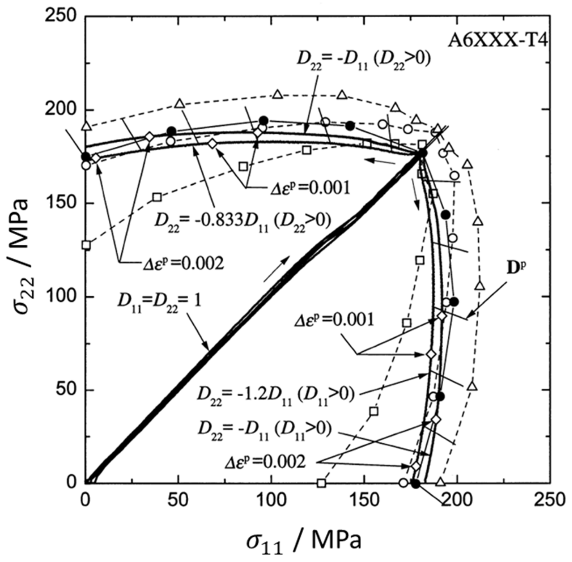
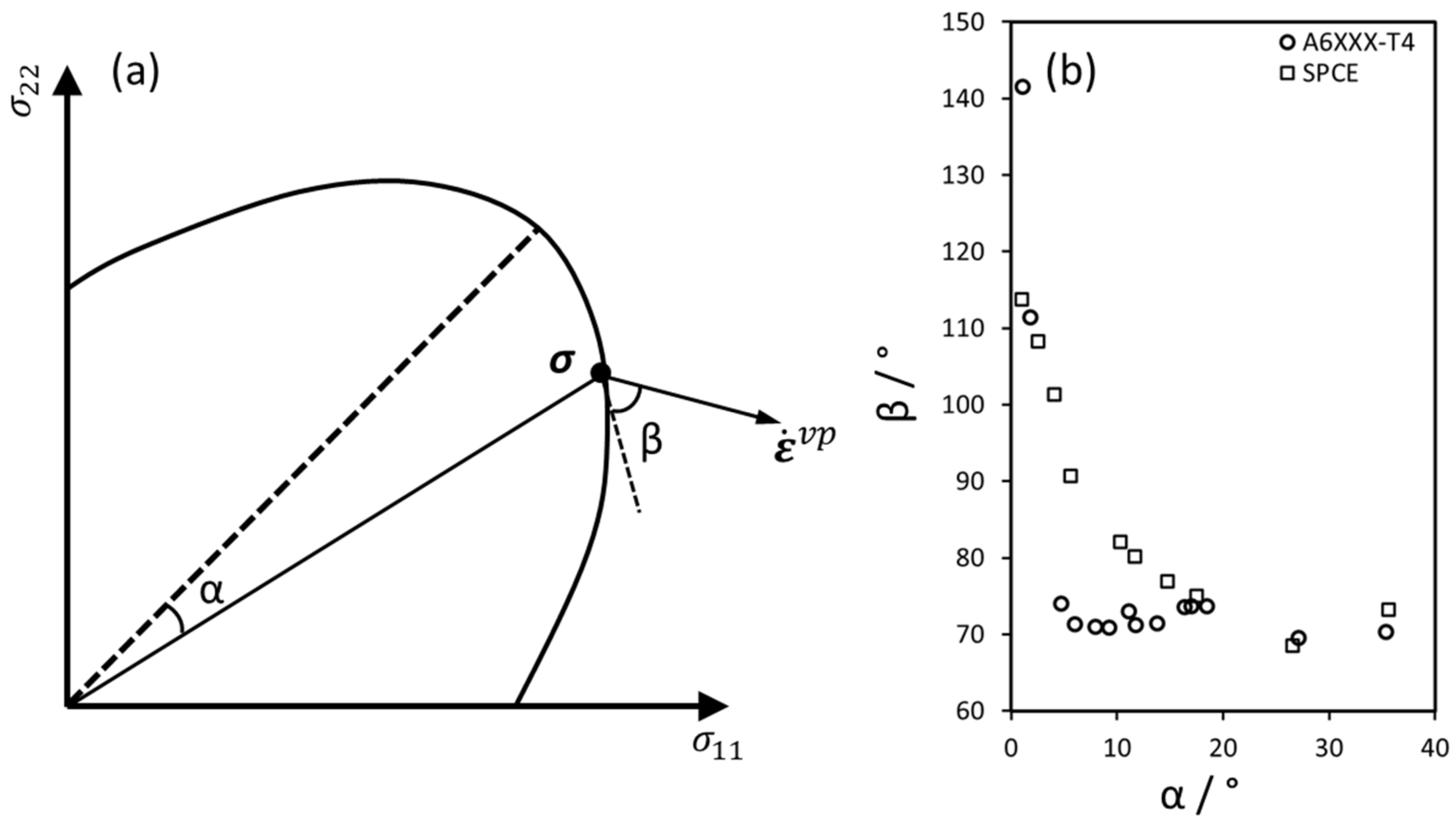
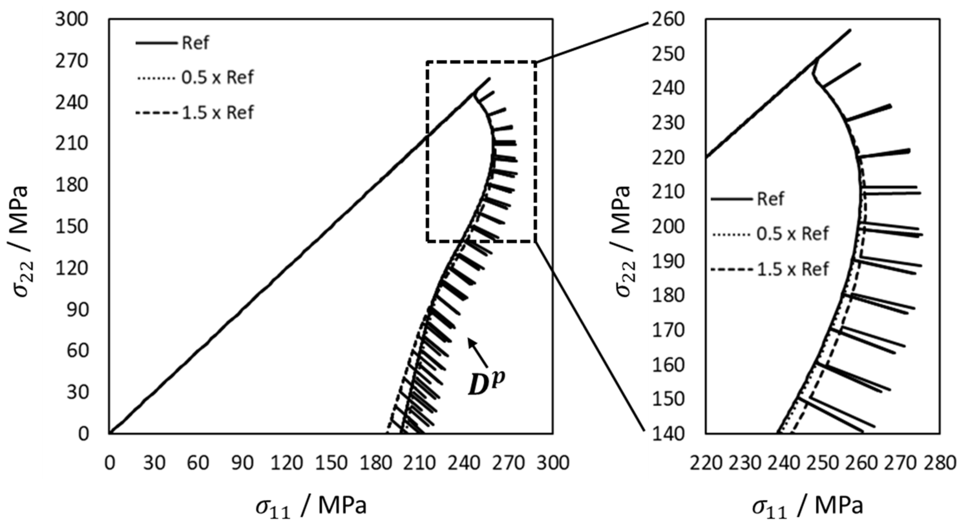
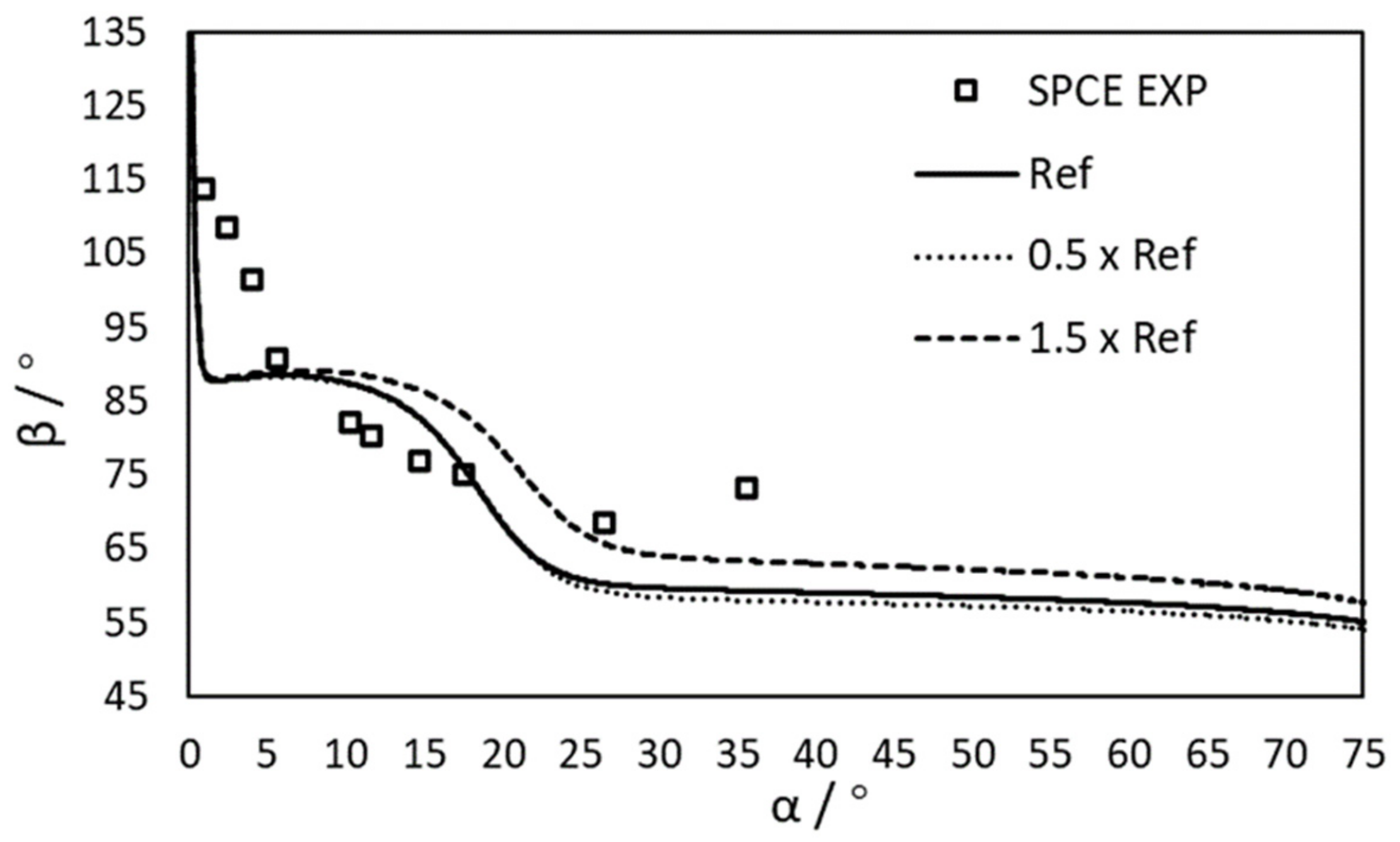
3.1. Simulations of Biaxial-to-Shear Experiments

In this section, a series of simulations of biaxial-to-shear tests have been performed using a self-developed program. The materials A6XXX-T4 aluminum and SPCE mild steel were described in detail in [32]. The biaxial-to-shear test consists of two-step loading processes as experimentally applied in [32]. The first loading step performed in the numerical investigations was an equi-biaxial loading formulated by ε ˙ 11 = ε ˙ 22   > 0. Once the biaxial strains reached the values ε 11 = ε 22 = 0.01 when the first loading was ended, the applied total strain rate was abruptly switched into ε ˙ 11 = ε ˙ 22 > 0 with ε ˙ 11 > 0 in the second loading path. Figure 1 illustrates the experimental investigations in [32], which determine the evolution of the yield locus by using biaxial-to-shear loading (solid lines). The dashed lines and symbols show the determined yield loci via loading–unloading–reloading method in [32]. The short black lines located on the subsequent yield surface, which determined via biaxial-to-shear the abrupt loading path change method, indicate the direction of plastic strain in the second loading path. Consequently, the evolution of stress trajectory is traced and the angle β , which describes the situation of normality after strain-path change is presented as a function of angle α , as illustrated in Figure 2.

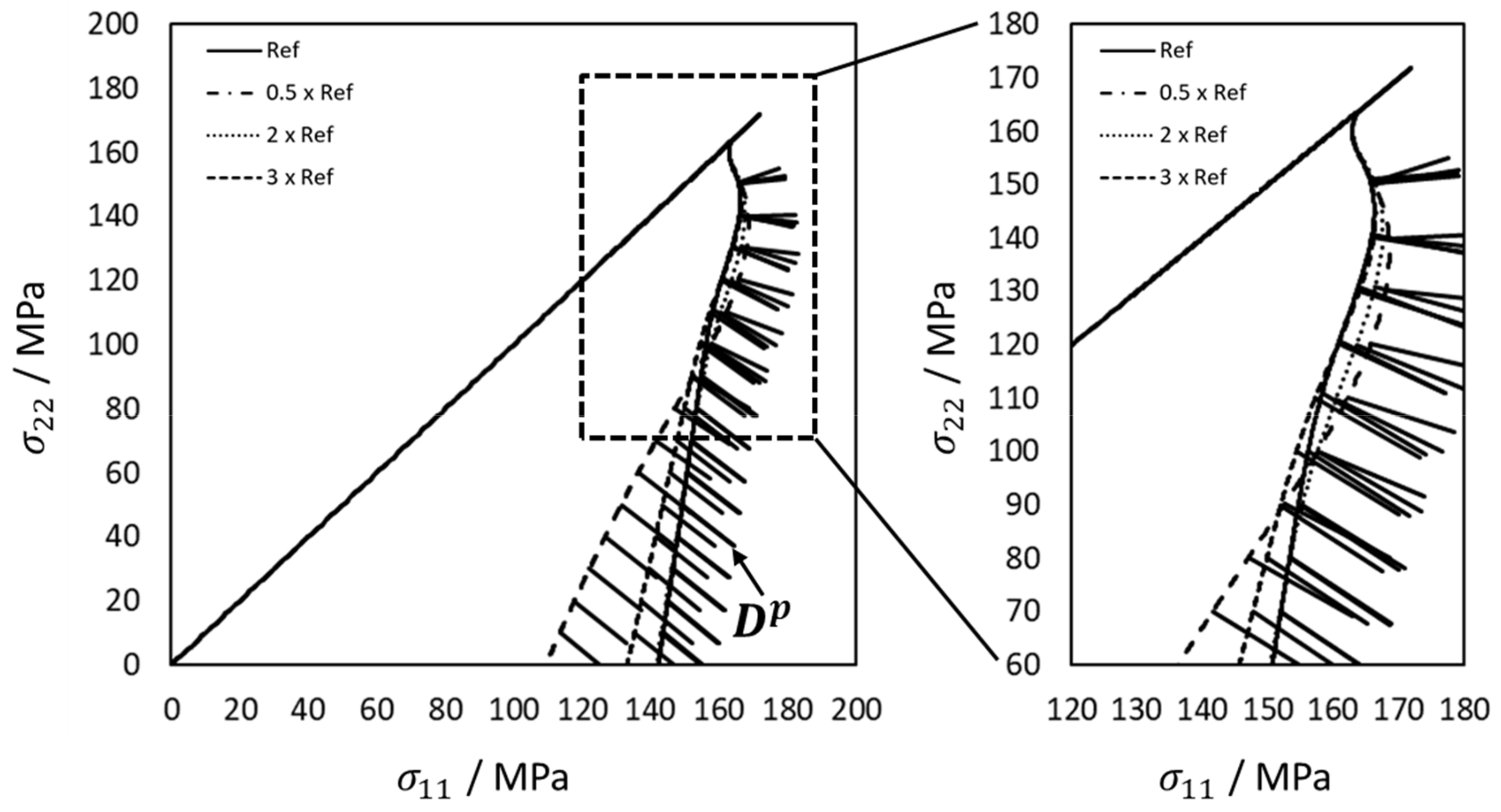
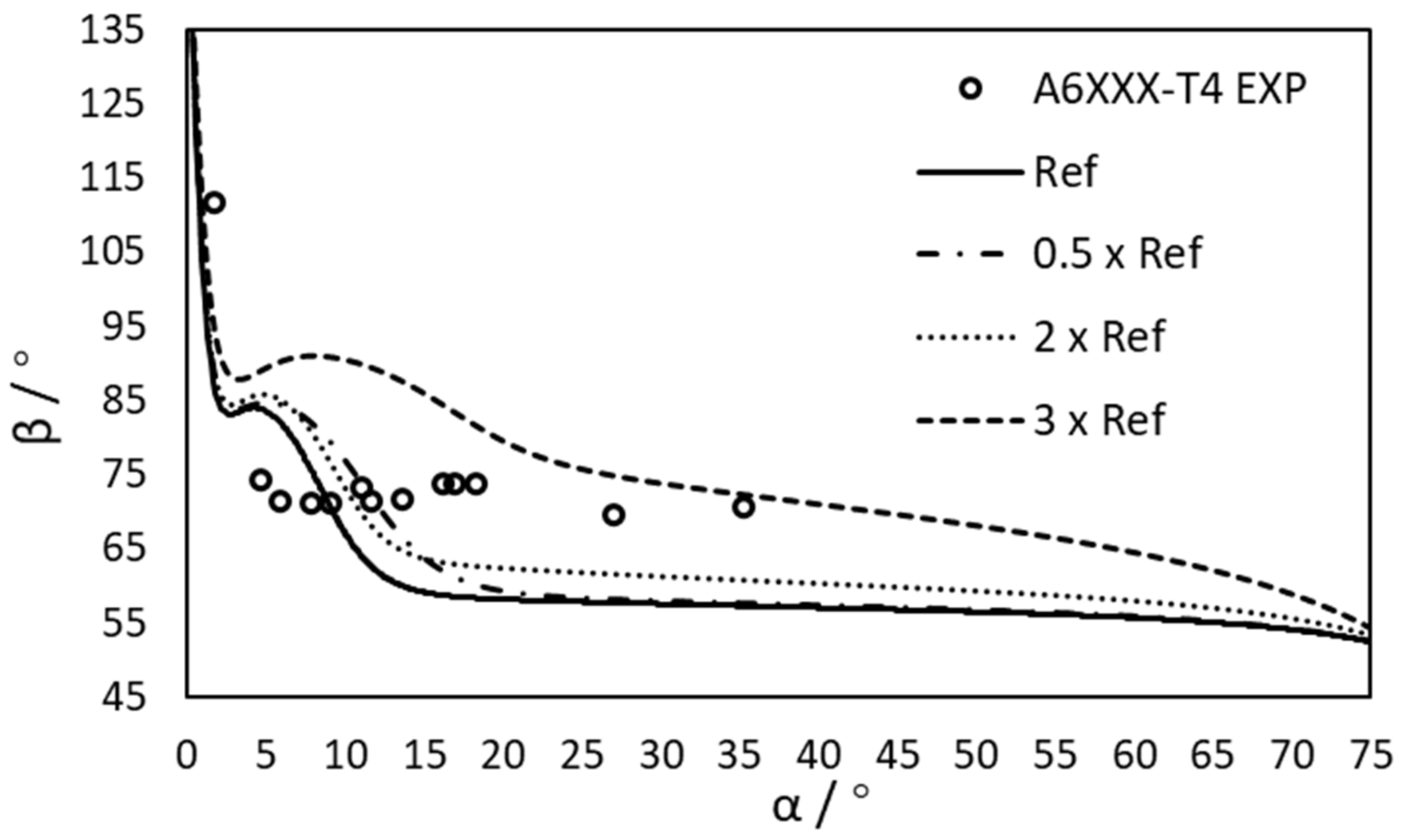
3.2. Effect of Cross Hardening

The material parameters of A6XXX-T4 aluminum and SPCE mild steel used in elasto-visco-plastic model for biaxial-to-shear simulation is given in Table 1, based on references [32,39]. The role of the cross-hardening effect on the yield locus evolution and normality loss was shown in Section 3.1. In Equation (6), the size of yield surface Y = Y 0 + R + f S where the contribution of the cross hardening is f S . To explore the effect of cross hardening on the apparent yield surface evolution and loss of normality after biaxial-to-shear loading path change, several simulations were performed for aluminum A6XXX-T4 and SPCE steel, respectively, by altering the parameters of the reference parameter set (Ref) by a selected factor (0.5 × Ref, 1.5 × Ref, 2 × Ref…). The reference material parameters of MTHH model that have been identified in [5], are given in Table 2 and Table 3 for the two investigated materials in this work.
The apparent yield locus evolution and normality loss after biaxial-to-shear loading path changes using different cross-hardening parameters for aluminum A6XXX-T4 are shown in Figure 3. The equi-biaxial tension stress reaches 163.3 MPa when the biaxial-to-shear loading path change occurs. It is worth noting that the biaxial stress states before the loading path change in the four simulations are rigorously identical, which is independent on the choice of different cross-hardening related parameters. Overall, the apparent shape of the four yield loci in the second loading path shows several differences as the accumulated plastic strain increases. For the largest cross-hardening case 3 × Ref, the apparent yield surface firstly deviates outwards (up to 5 MPa) and then shrinks inwards more rapidly, which induces a difference of around 25 MPa at σ 22 = 0 compared with the yield surface prediction using Ref values. However, for the cross-hardening case 2 × Ref, the predicted yield surface is almost the same as the referenced simulation result until the stress state in second loading path becomes ( σ 11   = 160 MPa, σ 22     = 120 MPa). Subsequently, the predicted yield surface using 2 × Ref cross-hardening gradually shrinks inwards, which deviates nearly 18 MPa when σ 22 =0. On the contrary, for the smaller cross-hardening case 0.5 × Ref, the predicted yield surface deviates slightly outwards (maximum 3MPa) compared with the Ref yield surface. Then, the 0.5 × Ref yield locus returns back to the Ref yield surface until the stress state in second loading path evolved at ( σ 11   = 170 MPa, σ 22   = 80 MPa), which causes the evolutions of two compared yield surfaces (0.5 × Ref, Ref) are almost identical despite the accumulated plastic strain level will be continuously increased. It is noteworthy that the trace of the stress history represented in Figure 3, only coincides with the yield surface in the particular case of isotropic hardening [12]. When more advanced models are used, this trace in stress space combines the effect of the yield surface shape and its evolution, even though the plastic stain cumulated during this transition stage is negligible [33]. These results were obtained with a simple symmetric von Moses yield surface, which highlight the necessity to consider not only the yield surface but also the hardening model when interpreting the apparent normality loss after biaxial-to-shear loading-path change.
The short black lines located on the yield surface after the biaxial-to-shear loading path change represent the direction of plastic strain. Figure 4 describes the evolution of β angle, which demonstrates that the apparent deviation from normality was affected by the different cross-hardening parameters. The angle β after the biaxial-to-shar strain-path change was 150.9° for all simulated cases, which was solely due to the viscous effect. In all simulations, angle β tended to converge to a value around 55° but the decrease in angle β was neither linear nor monotonic. The moment and rate of convergence of β angle strongly relied on the cross-hardening parameter. The α β curve using Ref value shows the largest rate of loss of normality. However, for the other three α β curves determined by (0.5 × Ref, 2 × Ref, 3 × Ref), the rate of loss of normality was decreased with the increasing of cross-hardening parameters. Compared with the experimental observed non-normality result β = 70° for aluminum A6XXX-T4, 3 × Ref predicted α β result underestimated the loss of normality when α was smaller than 35°. In turn, α β relationships given by (0.5 × Ref, Ref and 2 × Ref) overestimated the biaxial-to-shear strain-path change and induced non-normality. Clearly, the evolution of angle β for small α values (<15°…20°) needs deeper investigation. However, it appears that its subsequent evolution is strongly related to the cross-hardening behavior.
Similarly, the apparent yield locus evolution and normality loss situation after the biaxial-to-shear loading path changes, using the three groups’ cross-hardening parameters (0.5 × Ref, Ref, 1.5 × Ref) for mild steel SPCE, are given in Figure 5. The equi-biaxial tension stress is ( σ 11   = 248.8 MPa, σ 22   = 248.8 MPa) at the end of the first biaxial pre-loading point in all cases. Overall, the determined shape of the three apparent yield surfaces in the second loading path does not show significant differences as the accumulated plastic strain increasing. For the larger cross-hardening 1.5 × Ref, the determined yield surface slightly deviates outward (maximum 2 MPa), and then more severely evolves inward approximately 18 MPa, when σ 22   = 0 compared with the predicted yield surface via Ref value. The influence trend of smaller cross-hardening 0.5 × Ref on the yield surface evolution is different compared with that for the larger 1.5 × Ref. The predicted yield surface using 0.5 × Ref is nearly identical to the referenced simulation result until the stress state in second loading path becomes ( σ 11   = 220 MPa, σ 22   = 100 MPa). Soon after, the evolution of yield surface deviates slightly outwards maximum 3 MPa to the Ref yield surface at the moment σ 22   = 0.
Subsequently, the confrontations of normality loss between experimental and simulation results when using different cross-hardening parameters for steel SPCE is shown in Figure 6. The value of angle β after the biaxial-to-shear loading path change was 151.4° for all simulated cases. Overall, the decreasing tendency of angle β was neither linear nor monotonic, compared with the results for aluminum in Figure 4. In all simulations, angle β tended to converge to a value near 55° for 0.5 × Ref and 1.5 × Ref cases, and 58° for the 1.5 × Ref case. The α β curves using 0.5 × Ref and Ref values does not present obvious difference for the loss of normality, which means that the loss of normality is not sensitive to the smaller cross hardening values. The larger cross-hardening 1.5 × Ref determined α β curve indicates that the rate of loss of normality was decreased as the increasing of cross hardening values. Furthermore, the predicted α β results from 0.5 × Ref and Ref are comparative closer to experimental results among the three predicted curves. In addition, all of these three cross-hardening cases overestimated the biaxial-to-shear strain-path change induced loss of normality.

4. Conclusions

In this paper, the influence of cross hardening on the apparent yield locus evolution and normality loss after biaxial-to-shear loading path change was discussed. An elasto-visco-plastic constitutive model framework using a modified Teodosiu–Hu hardening model was employed. The apparent non-normality observed in two-step loading investigations was shown to depend on the cross-hardening responses of two materials within a classical plasticity modeling context. The cross hardening had a significant influence on the evolution of the β angle and led to results showing some agreements with the experiments in the literature, in particular for α angles larger than 20°. It can be concluded that cross hardening has an important effect on the apparent yield locus evolution and normality loss. The FE implementation of the proposed generic model is expected to improve forming process predictions such as springback and forming limits, etc.

Author Contributions

Conceptualization, T.B. and Y.Y.; methodology, T.B.; software, Y.Y.; validation, T.B., Y.Y., C.B.; investigation, Y.Y.; resources, C.B.; data curation, Y.Y.; writing—original draft preparation, Y.Y.; writing—review and editing, T.B, Y.Y.; visualization, Y.Y.; supervision, T.B.; project administration, C.B.; funding acquisition, C.B. All authors have read and agreed to the published version of the manuscript.

Funding

The PhD grand of YY during this work was funded by the China Scholarship Council (CSC N° 201606020110).

Conflicts of Interest

The authors declare no conflict of interest.

References

  1. Li, S.; Hoferlin, E.; Van Bael, A.; Van Houtte, P.; Teodosiu, C. Finite element modeling of plastic anisotropy induced by texture and strain-path change. Int. J. Plast. 2003, 19, 647–674. [Google Scholar] [CrossRef]
  2. Hu, W. Constitutive modeling of orthotropic sheet metals by presenting hardening-induced anisotropy. Int. J. Plast. 2007, 23, 620–639. [Google Scholar] [CrossRef]
  3. Mánik, T.; Holmedal, B.; Hopperstad, O.S. Strain-path change induced transients in flow stress, work hardening and r-values in aluminum. Int. J. Plast. 2015, 69, 1–20. [Google Scholar] [CrossRef] [Green Version]
  4. González-Arévalo, N.; Velázquez, J.; Díaz-Cruz, M.; Cervantes-Tobón, A.; Terán, G.; Hernández-Sanchez, E.; Capula-Colindres, S. Influence of aging steel on pipeline burst pressure prediction and its impact on failure probability estimation. Eng. Fail. Anal. 2021, 120, 104950. [Google Scholar] [CrossRef]
  5. Haddadi, H.; Bouvier, S.; Banu, M.; Maier, C.; Teodosiu, C. Towards an accurate description of the anisotropic behaviour of sheet metals under large plastic deformations: Modelling, numerical analysis and identification. Int. J. Plast. 2006, 22, 2226–2271. [Google Scholar] [CrossRef]
  6. Bouvier, S.; Alves, J.; Oliveira, M.; Menezes, L. Modelling of anisotropic work-hardening behaviour of metallic materials subjected to strain-path changes. Comput. Mater. Sci. 2005, 32, 301–315. [Google Scholar]
  7. Wang, J.; Levkovitch, V.; Svendsen, B. Modeling and simulation of directional hardening in metals during non-proportional loading. J. Mater. Process. Technol. 2006, 177, 430–432. [Google Scholar] [CrossRef]
  8. Thuillier, S.; Manach, P.-Y. Comparison of the work-hardening of metallic sheets using tensile and shear strain paths. Int. J. Plast. 2009, 25, 733–751. [Google Scholar] [CrossRef]
  9. Vincze, G.; Barlat, F.; Rauch, E.F.; Tomé, C.N.; Butuc, M.C.; Grácio, J.J. Experiments and modeling of low carbon steel sheet subjected to double strain path changes. Metall. Mater. Trans. A 2013, 44, 4475–4479. [Google Scholar] [CrossRef] [Green Version]
  10. Barlat, F.; Vincze, G.; Grácio, J.; Lee, M.-G.; Rauch, E.; Tomé, C. Enhancements of homogenous anisotropic hardening model and application to mild and dual-phase steels. Int. J. Plast. 2014, 58, 201–218. [Google Scholar] [CrossRef]
  11. Chen, Z.; Zhao, J.; Fang, G. Finite element modeling for deep-drawing of aluminum alloy sheet 6014-T4 using anisotropic yield and non-AFR models. Int. J. Adv. Manuf. Technol. 2019, 104, 535–549. [Google Scholar] [CrossRef]
  12. Kuroda, M.; Tvergaard, V. Use of abrupt strain path change for determining subsequent yield surface: Illustrations of basic idea. Acta Mater. 1999, 47, 3879–3890. [Google Scholar] [CrossRef]
  13. Khan, A.S.; Kazmi, R.; Pandey, A.; Stoughton, T. Evolution of subsequent yield surfaces and elastic constants with finite plastic deformation. Part-I: A very low work hardening aluminum alloy (Al6061-T6511). Int. J. Plast. 2009, 25, 1611–1625. [Google Scholar] [CrossRef]
  14. Khan, A.S.; Pandey, A.; Stoughton, T. Evolution of subsequent yield surfaces and elastic constants with finite plastic deformation. Part II: A very high work hardening aluminum alloy (annealed 1100 Al). Int. J. Plast. 2010, 26, 1421–1431. [Google Scholar] [CrossRef]
  15. Khan, A.S.; Pandey, A.; Stoughton, T. Evolution of subsequent yield surfaces and elastic constants with finite plastic deformation. Part III: Yield surface in tension–tension stress space (Al 6061–T 6511 and annealed 1100 Al). Int. J. Plast. 2010, 26, 1432–1441. [Google Scholar] [CrossRef]
  16. Iftikhar, A.; Khan, A.S. The Evolution of Yield Loci with Finite Plastic Deformation along Proportional & Non-proportional Loading Paths in an Annealed Extruded AZ31 Magnesium Alloy. Int. J. Plast. 2021, 143, 103007. [Google Scholar]
  17. Hu, G.; Zhang, K.; Huang, S.; Ju, J.-W.W. Yield surfaces and plastic flow of 45 steel under tension-torsion loading paths. Acta Mech. Solida Sin. 2012, 25, 348–360. [Google Scholar] [CrossRef]
  18. Lu, D.; Zhang, K.; Hu, G.; Lan, Y.; Chang, Y. Investigation of Yield Surfaces Evolution for Polycrystalline Aluminum after Pre-Cyclic Loading by Experiment and Crystal Plasticity Simulation. Materials 2020, 13, 3069. [Google Scholar] [CrossRef]
  19. Gotoh, M. A class of plastic constitutive equations with vertex effect—I. General theory. Int. J. Solids Struct. 1985, 21, 1101–1116. [Google Scholar] [CrossRef]
  20. Gotoh, M. A class of plastic constitutive equations with vertex effect—II. Discussions on the simplest form. Int. J. Solids Struct. 1985, 21, 1117–1129. [Google Scholar] [CrossRef]
  21. Hughes, T.J.; Shakib, F. Pseudo-corner theory: A simple enhancement of J2-flow theory for applications involving non-proportional loading. Eng. Comput. 1986, 3, 116–120. [Google Scholar] [CrossRef]
  22. Simo, J. A J2-flow theory exhibiting a corner-like effect and suitable for large-scale computation. Comput. Methods Appl. Mech. Eng. 1987, 62, 169–194. [Google Scholar] [CrossRef]
  23. Kuroda, M.; Tvergaard, V. Plastic spin associated with a non-normality theory of plasticity. Eur. J. Mech.-ASolids 2001, 20, 893–905. [Google Scholar] [CrossRef]
  24. Kuroda, M.; Tvergaard, V. A phenomenological plasticity model with non-normality effects representing observations in crystal plasticity. J. Mech. Phys. Solids 2001, 49, 1239–1263. [Google Scholar] [CrossRef]
  25. Kuroda, M. A higher-order strain gradient plasticity theory with a corner-like effect. Int. J. Solids Struct. 2015, 58, 62–72. [Google Scholar] [CrossRef]
  26. Stoughton, T.B. A non-associated flow rule for sheet metal forming. Int. J. Plast. 2002, 18, 687–714. [Google Scholar] [CrossRef]
  27. Cvitanić, V.; Vlak, F.; Lozina, Ž. A finite element formulation based on non-associated plasticity for sheet metal forming. Int. J. Plast. 2008, 24, 646–687. [Google Scholar] [CrossRef]
  28. Safaei, M.; Lee, M.-G.; De Waele, W. Evaluation of stress integration algorithms for elastic–plastic constitutive models based on associated and non-associated flow rules. Comput. Methods Appl. Mech. Eng. 2015, 295, 414–445. [Google Scholar] [CrossRef]
  29. Taherizadeh, A.; Green, D.E.; Yoon, J.W. Evaluation of advanced anisotropic models with mixed hardening for general associated and non-associated flow metal plasticity. Int. J. Plast. 2011, 27, 1781–1802. [Google Scholar] [CrossRef]
  30. Lee, E.-H.; Stoughton, T.B.; Yoon, J.W. A yield criterion through coupling of quadratic and non-quadratic functions for anisotropic hardening with non-associated flow rule. Int. J. Plast. 2017, 99, 120–143. [Google Scholar] [CrossRef]
  31. Park, N.; Stoughton, T.B.; Yoon, J.W. A criterion for general description of anisotropic hardening considering strength differential effect with non-associated flow rule. Int. J. Plast. 2019, 121, 76–100. [Google Scholar] [CrossRef]
  32. Kuwabara, T.; Kuroda, M.; Tvergaard, V.; Nomura, K. Use of abrupt strain path change for determining subsequent yield surface: Experimental study with metal sheets. Acta Mater. 2000, 48, 2071–2079. [Google Scholar] [CrossRef]
  33. Yang, Y.; Balan, T. Prediction of the yield surface evolution and some apparent non-normality effects after abrupt strain-path change using classical plasticity. Int. J. Plast. 2019, 119, 331–343. [Google Scholar] [CrossRef]
  34. Yoshida, K.; Okada, N. Plastic flow behavior of fcc polycrystal subjected to nonlinear loadings over large strain range. Int. J. Plast. 2020, 127, 102639. [Google Scholar] [CrossRef]
  35. Hama, T.; Yagi, S.; Tatsukawa, K.; Maeda, Y.; Maeda, Y.; Takuda, H. Evolution of plastic deformation behavior upon strain-path changes in an A6022-T4 Al alloy sheet. Int. J. Plast. 2021, 137, 102913. [Google Scholar] [CrossRef]
  36. Teodosiu, C.; Hu, Z. Evolution of the intragranular microstructure at moderate and large strains: Modelling and computational significance. Simul. Mater. Process Theory Methods Appl. 1995, 173–182. [Google Scholar]
  37. Haddag, B.; Balan, T.; Abed-Meraim, F. Investigation of advanced strain-path dependent material models for sheet metal forming simulations. Int. J. Plast. 2007, 23, 951–979. [Google Scholar] [CrossRef] [Green Version]
  38. Yang, Y.; Vincze, G.; Baudouin, C.; Chalal, H.; Balan, T. Strain-path dependent hardening models with rigorously identical predictions under monotonic loading. Mech. Res. Commun. 2021, 114, 103615. [Google Scholar] [CrossRef]
  39. Pipard, J.-M.; Balan, T.; Abed-Meraim, F.; Lemoine, X. Elasto-visco-plastic modeling of mild steels for sheet forming applications over a large range of strain rates. Int. J. Solids Struct. 2013, 50, 2691–2700. [Google Scholar] [CrossRef]
Figure 1. Experimental results determining the evolution of the yield locus by using biaxial-to-shear loading (solid lines). Dashed lines/symbols present the yield loci vis loading–unloading–reloading method in [32] for aluminum alloy A6XXX-T4.
Symmetry 14 00142 g001
Figure 2. Schematic illustration of (a) apparent normality loss after biaxial-to-shear loading path change and definition of angles α and β; (b) experimental observation of normality loss for aluminum A6XXX-T4 and mild steel SPCE in [32].
Symmetry 14 00142 g002
Figure 3. Prediction of yield surface evolution and apparent loss of normality situation after biaxial-to-shear loading path changes with using different cross hardening parameters for aluminum A6XXX-T4.
Symmetry 14 00142 g003
Figure 4. Normality loss confrontations of experimental and simulation results after biaxial-to-shear loading path changes with using different cross hardening parameters for aluminum A6XXX-T4.
Symmetry 14 00142 g004
Figure 5. Prediction of apparent yield locus evolution and normality loss situation after biaxial-to-shear loading path changes with using different cross hardening parameters for steel SPCE.
Symmetry 14 00142 g005
Figure 6. Normality loss confrontations of experimental and simulation results after biaxial-to-shear loading path changes with using different cross hardening parameters for steel SPCE.
Symmetry 14 00142 g006
Table 1. Mechanical parameters of SPCE and A6XXX-T4 used in elasto-visco-plastic model for biaxial-to-shear simulation [32,39].
Materials E (GPa) Y 0   ( MPa ) ε ˙ # k #
A6XXX-T4701250.120
SPCE2101800.236
Table 2. Cross-hardening parameters used in the investigations of the apparent yield locus evolution and normality loss for aluminum A6XXX-T4.
Parameters K . (MPa) ε 0 n C x X 0   ( MPa ) f C S D C S L n L S s a t   ( MPa ) C P n p r
Ref6000.020.41001500.43.91.102472.2281.9
0.5 × Ref0.21.950.550123.51.1140.95
2 × Ref0.87.82.204944.4563.8
3 × Ref1.211.73.307416.6845.7
Table 3. Cross-hardening parameters used in the investigations of the apparent yield locus evolution and normality loss for steel SPCE.
Parameters K (MPa) ε 0 n C x X 0   ( MPa ) f C S D C S L n L S s a t   ( MPa ) C P n p r
Ref5200.0040.2902000.82.851.205650.678900.8
0.5 × Ref0.41.430.60282.50.344450.4
1.5 × Ref1.24.282.80847.5113351.2
Publisher’s Note: MDPI stays neutral with regard to jurisdictional claims in published maps and institutional affiliations.

