A Heuristic Integrated Scheduling Algorithm via Processing Characteristics of Various Machines

Abstract

Complex products with a tree-like structure usually have an asymmetric structure. Therefore, in order to avoid the separation of equipment and operation correlation during the scheduling, the structural attributes of products and the use of equipment resources should be fully considered. However, this feature is ignored in the current research works on the scheduling of multi-variety and small batch products. This leads to increased idle time for equipment and an extended makespan for products. To avoid this situation, a heuristic integrated scheduling algorithm via processing characteristics of various machines (HIS-PCVM) is proposed. In the integrated scheduling, the algorithm first divides the equipment into two categories: the special equipment and the general equipment according to the resources of the production scheduling system. Then, different scheduling methods are designed according to the equipment categories. The makespan of the product is further optimized through various combination methods. Moreover, the constraint audit strategy to guarantee the constraint relationship between the operations is optimized. The earliest scheduling time strategy is proposed to improve the parallelism and serial tightness of the operations. These strategies reduce the idle time of equipment effectively. Experimental results show that the proposed algorithm has a better application effect in reducing the makespan of complex products, both with asymmetric structures and symmetric structures. This also shows that the algorithm is effective in improving the utilization rate of equipment.

1. Introduction

As a key link of the manufacturing system, the scheduling problem has always attracted widespread attention from the academic circles. An efficient scheduling system can not only reduce the makespan of product manufacturing but also improve the economic and social benefits of the enterprises. With the development of intelligent technology and the change of social demand (see Refs. [1,2,3,4,5]), the structure of scheduling products is also diversified (see Refs. [6,7,8,9,10]). In 2020, some authors [11,12] carried out in-depth research on symmetric scheduling. Other authors (see Refs. [13,14,15,16,17]) carried out in-depth research on asymmetric scheduling.

However, with the diversification of product manufacturing and personalized demand, the product scheduling problem of small batch products with a complex processing structure is becoming more and more prominent. Different from the flow-shop scheduling problem and the job-shop scheduling problem in the traditional industry, Xie put forward a third type of scheduling mode, that is, integrated scheduling. This is a scheduling mode for the production of multi-variety and small batch products. Under this mode, the processing stage and the assembly stage of complex products with symmetric or asymmetric tree structures are scheduled synchronously [18]. Scholars have conducted a thorough study on this scheduling mode and obtained abundant results. Nowadays, integrated scheduling is widely used in many fields (see Refs. [19,20,21,22,23,24,25,26,27,28,29,30,31,32,33,34]). For example, for the flexible integrated scheduling problem, Yang D. et al. [19] proposed an improved artificial bee colony algorithm considering MSE with two new strategies. Similarly, based on the intelligent algorithms, Gao Y. et al. [20] proposed an algorithm based on the priority constraint table to solve the problem of the task scheduling result being affected by a state change of the computing system. For the scheduling mathematical models, Defersha F. et al. [21] proposed a mathematical model for a new setup operator constrained flexible job-shop scheduling problem. Based on the time-selected scheduling idea, Zhang X. et al. [27] proposed an algorithm to consider the precision of serial operations. Zhou W. et al. [28] proposed an algorithm that considers the hierarchical scheduling order for the integrated scheduling problem with a large number of operations in the same layer. For the scheduling solution approaches, Papatya S. et al. [29] proposed a new formulation for this problem and compared it with a recent formulation. Based on the key machine’s compact procedures, Xie and Zheng [32] proposed a dynamical integrated scheduling algorithm. Based on Job-Shop Scheduling Problem, Xie and Yang et al. [33] proposed an algorithm constructed a manufacturing tree based on JSSP. However, in the study of operation optimization, if the advantage of the leaf node operations on the short path is to start processing earlier, then the first fit scheduling strategy will be invalid, regardless of whether it is a long path strategy or a strategy based on the successor operations. In the study of machine optimization, if there are competitive operations for a machine with different processing characteristics, the short time strategy will fail, and the performance of the longitudinal optimization scheduling will be poor. Thus, many idle time periods will appear on the special equipment.

Based on the above analysis, a heuristic integrated scheduling algorithm via processing characteristics of various machines (HIS-PCVM) is proposed to minimize the makespan. The proposed algorithm divides the equipment into special equipment and general equipment according to the processing characteristics. Three types of scheduling strategies are designed for the resources of different types of equipment. In terms of vertical optimization, the operation serial tightness is further improved. In terms of horizontal optimization, the machine idle time is effectively reduced. In conclusion, it achieves the optimization effect of reducing the overall makespan of complex products and improves the machine utilization rate.

The rest of the paper is arranged as follows. In the next section, a detailed description of the integrated scheduling problem of complex products is given. Then, Section 3 describes the design process of the proposed algorithm in detail. The superiority of the proposed algorithm is verified by comparative experiments of symmetric and asymmetric complex product scheduling in Section 4. Finally, in Section 5, we draw some conclusions and prospects for future research work.

2. Problem Analysis and Description

The integrated scheduling problem can be described as a single complex tree-structured product consisting of n operations needs to be processed on m machines. The specific requirements are as follows:

(1)

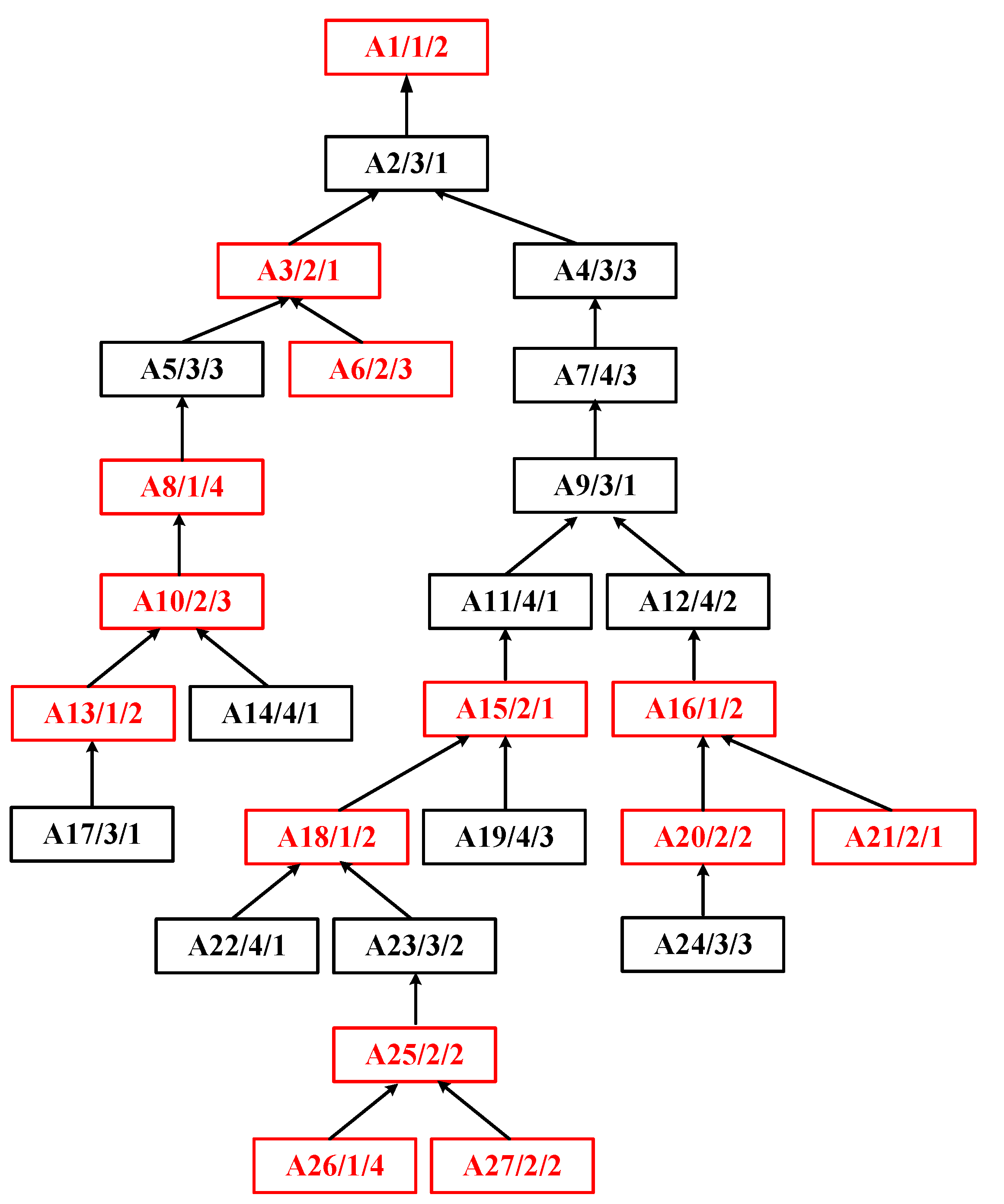
Each operation has three elements: the operation number, the machine number, and the processing time;

(2)

Each occupied machine has two properties: the time certainty and the processing continuity;

(3)

Except for leaf node operations, the sufficient and necessary condition of each operation is that all of its immediate predecessor operations are completed;

(4)

The end time of the last operation is the total processing time of the product.

To shorten the makespan of production, it is necessary to determine the reasonable starting time of each operation. In integrated scheduling, the leaf node operations and root node operation only have the immediate successor operations or the immediate predecessor operations. The other node operations have both the constraints with their immediate successor operations and their immediate predecessor operations. Moreover, each operation can be started only when its immediate predecessor operations (group) are finished.

The scheduling goal of the problem is to make the product’s makespan as short as possible. The mathematical model of this problem can be described as follows.

The optimization objective is

$$\underset{i\in O}{\max }\{C_i=P_i+S_i\}$$

(1)

The constraint is

$$S_i+P_i\le S_j,\forall (i,j)\in R$$

(2)

$$S_i+P_i-(1-y_{ij})L\le S_j,\forall i,j\in O,i\ne j$$

(3)

$$y_i{}_j=\{\begin{array}{cc}1& \mathrm{if} i \mathrm{processes} \mathrm{earlier} \mathrm{than} j \mathrm{on} \mathrm{the} \mathrm{same} \mathrm{machine} \\ 0& \mathrm{otherwise}\end{array}$$

(4)

$$S_i\ge 0,P_i\ge 0$$

(5)

This MIP model uses a binary variable y_ij to indicate whether operation i is allocated earlier to the same machine as operation j. For example, y_ij = 1 and y_ji = 0 mean that operation i processes before j on the same machine. For each operation, if its starting time is S_i, then after processing time P_i on its corresponding machine, its completion time is C_i. The scheduling goal is to shorten the completion time of the final operation, as shown in Formula (1). Constraint (2) says that each operation j must be stated after its immediate predecessor operation i finishes, and the relation set R = {(i, j) |if i is the immediate predecessor of j} is used to store the constraint relationships. It represents the precedence constraints. Constraint (3) guarantees that operations on the same machine cannot be processed at the same time, and L is a large positive constant. Formulas (3) and (4) give the boundary of y_ij, S_i, and P_i to make them significant in practice.

In this paper, as we divide the machines into three different types, all the operations are scheduled according to the types of their machines. We use three operation sequences to restore the operations with an initial order, which can be obtained by the corresponding strategies. The mathematical expressions of the three operation sequences are as follows.

The multi-operation machine scheduling sequence

$$Q_{MOM}=\{i_1,i_2,i_3,\dots ,i_s|\forall i_l\in MOM,l=1,2,\dots ,s,s\le n\}$$

(6)

$$i_1\succ i_2,\mathrm{if} L_{i_1}\vee L_{i_2}=L_{i_1},L_{i_1}\ne L_{i_2}\mathrm{or} {\alpha }_{i_1}\vee {\alpha }_{i_2}={\alpha }_{i_1},L_{i_1}=L_{i_2}$$

(7)

The more-time machine scheduling sequence

$$Q_{MTM}=\{i_1,i_2,i_3,\dots ,i_t|\forall i_l\in MTM,l=1,2,\dots ,t,t\le n\}$$

(8)

$$i_1\succ i_2,\mathrm{if} L_{i_1}\vee L_{i_2}=L_{i_1},L_{i_1}\ne L_{i_2}\mathrm{or} D_{i_1}\vee D_{i_2}=D_{i_1},L_{i_1}=L_{i_2}$$

(9)

The general machine scheduling sequence

$$Q_{GM}=\{i_1,i_2,i_3,\dots ,i_g|\forall i_l\in GM,l=1,2,\dots ,g,g\le n\}$$

(10)

$$i_1\succ i_2,\mathrm{if} P{V}_{i_1}\vee P{V}_{i_2}=P{V}_{i_1},P{V}_{i_1}\ne P{V}_{i_2}\mathrm{or} L_{i_1}\vee L_{i_2}=L_{i_1},P{V}_{i_1}=P{V}_{i_2}\mathrm{or} D_{i_1}\vee D_{i_2}=D_{i_1},L_{i_1}=L_{i_2}$$

(11)

$$s+t+g=n$$

(12)

MOM indicates the operation set of multi-operation machines. It contains s operations. Formula (6) represents the scheduling sequence Q_MOM of all the operations in MOM, and the subscript means the schedule number of each operation in the sequence. For example, i₁₁ is the 11th operation, which will be scheduled on multi-operation machines. Formula (7) says the reason for operation i₁ is scheduled earlier than i₂. As the operations in MOM are scheduled by the strategy of layer priority and the strategy of leaf node first, if operation i₁ is scheduled earlier than i₂, the layer priority $L_{i_1}$ must be larger than $L_{i_2}$. If the layer priorities are the same, the binary leaf node judge parameter ${\alpha }_{i_1}$ should be the larger one. If ${\alpha }_{i_1}=1$, operation i₁ is a leaf node. Formula (8) represents the scheduling sequence Q_MTM of all the t operations in MTM. Additionally, the operations in MTM are scheduled by the strategy of layer priority and the strategy of the highest constraint degree first. Formula (9) explains why operation i₁ is scheduled earlier than i₂. Similar to Formula (7), when the layer priorities are the same, the constraint degree $D_{i_1}$ must be larger than $D_{i_2}$. Formula (10) represents the scheduling sequence Q_GM of all the g operations in GM. Additionally, the operations in GM are scheduled by the strategy of large path value, the strategy of layer priority, and the strategy of the highest constraint degree first. Additionally, Formula (11) explains why operation i₁ is scheduled earlier than i₂. If operation i₁ has a larger path value $P_{i_1}$, higher layer priority $L_{i_1}$, or larger constraint degree $D_{i_1}$, then operation i₁ is more preferred. Formula (12) says that the total number of these three operation sets must be equal to the total number of the operations of the product.

3. Algorithm Design Ideas

3.1. Relevant Definitions

Definition 1 ([33]).

The operation priority. The scheduling order of an operation is defined as the operation priority of it. It depends on the layer at which the operation is located. For example, assuming that a process tree has n layers, and the priority of the root node operation is defined as one, then, the priorities of all the successor node operations of the root node operation are defined as two, and the operations at the same layer are regarded as the brother nodes. The priorities of all nodes at the nth layer are defined as n. The priority of the root node is basically defined as the lowest, and the highest priority is the operation at the nth layer.

Definition 2.

The multi-operation machine. The machine with the largest number of operations to be processed is defined as the multi-operation machine. It belongs to the special equipment.

Definition 3.

The more-time machine. In integrated scheduling, Ref. [28] first defined the machine with the longest scheduling time to process the operations as the key machine. However, in this paper, such machine is defined as the more-time machine. It belongs to the special equipment.

Definition 4.

The general machine. In integrated scheduling, these are machines other than multi-operation machines and more-time machines. They belong to the general equipment.

Definition 5.

The earliest scheduling time. For each operation, the end time of its immediate predecessor operation (group) is defined as the earliest scheduling time for it.

Definition 6.

The path value. The processing time of each operation in a process tree is defined as the path value between it and its immediate successor operations.

Definition 7.

The constraint degree. For an operation, the number of its immediate predecessors and immediate successors is defined as the constraint degree of it.

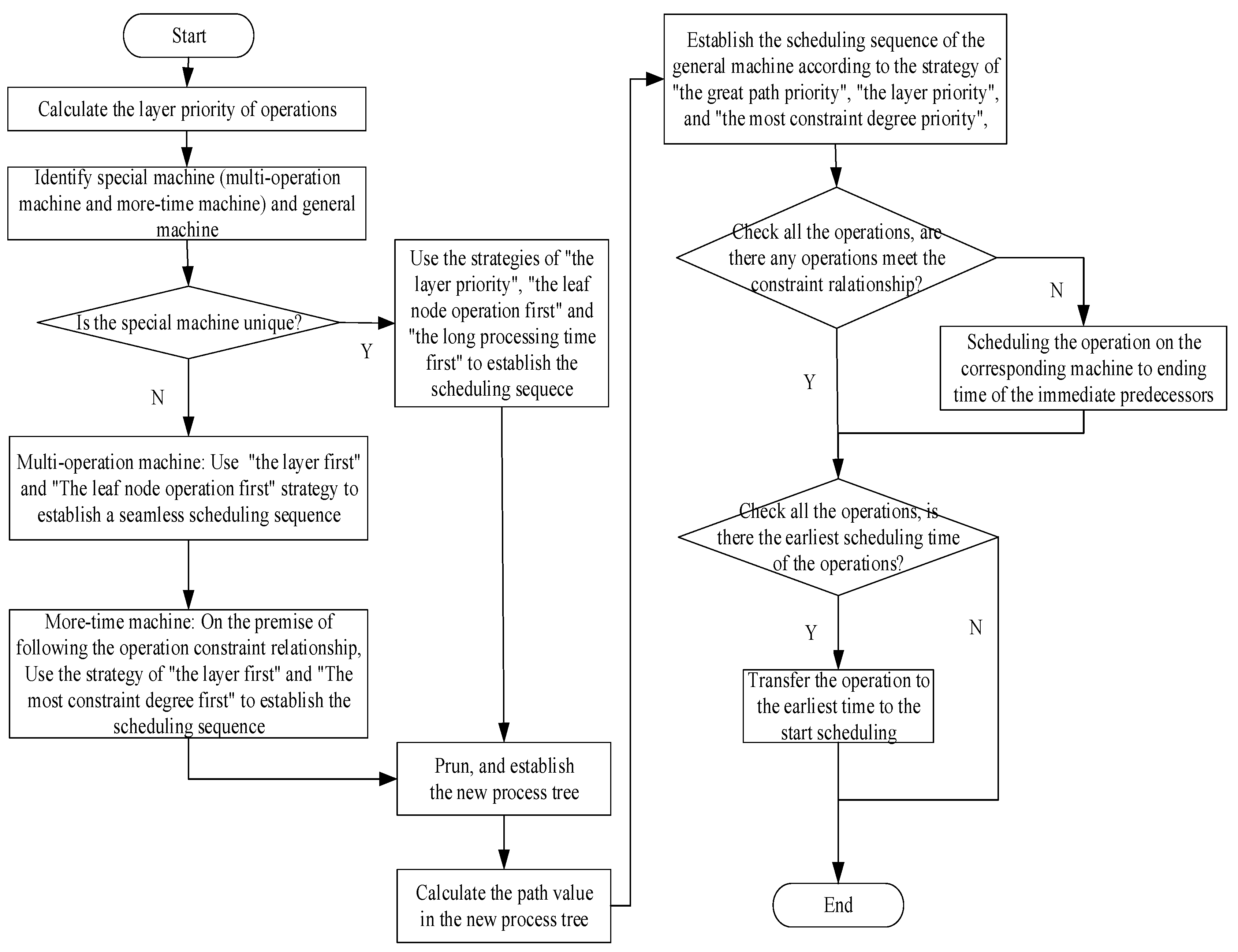
3.2. Description of the Algorithm

Since the scheduling effect of the operations on special equipment plays an important role in the overall optimization of integrated scheduling, in this paper, we proposed a combined scheduling mechanism for the multi-operation machine, the more-time machine, and the general machine. To begin with, according to the machine characteristics of the production scheduling system, the equipment is divided into special equipment (the multi-operation machine, the more-time machine) and general equipment (the general machine). In addition, when the special equipment is not unique, the layer priority strategy and the leaf node first strategy are adopted for the multi-operation machine to schedule each operation seamlessly. Meanwhile, the strategies of “the layer priority” and “the highest constraint degree first” are used to schedule each operation on the more-time machines. When the special equipment is unique, the strategies of “the layer priority”, “the leaf nodes first”, and “the long self-processing time first” are adopted to establish the scheduling sequence of the special machine. Moreover, on the general equipment, each operation is scheduled by using the methods of “the great path value first”, “the layer priority”, and “the great constraint degree first” in turn. Finally, each scheduled operation is adjusted by using the constraint audit strategy and the earliest scheduling time strategy to complete the production of the complex product.

The specific implementation steps are as follows:

Step1: According to the structure characteristics of the process tree of the complex product, confirm the layer number of the process tree and calculate the layer priority of each operation;

Step2: Confirm the special equipment and the general equipment according to the machine resources;

Step3: Confirm whether the special equipment is unique. If it is unique, go to Step4. Otherwise, go to Step7;

Step4: On the special machine, use the strategies of “the layer priority”, “the leaf node operation first”, and “the long processing time first” to establish the scheduling sequence;

Step5: On the basis of the process tree, cut off the scheduled operations and establish a new process tree;

Step6: Calculate the path value from each operation to the root node operation in the new process tree in turn and establish the scheduling sequence of the general machine according to the strategy of “the highest path value priority”, “the layer priority”, and “the highest constraint degree priority”. Turn to Step9;

Step7: For the multi-operation machine, use the strategies of “the layer priority” and “the leaf node operation first” to establish a seamless scheduling operation sequence;

Step8: For the more-time machine, on the premise of following the operation constraint relationship, use the strategy of “the layer priority” and the strategy of “the great constraint degree priority” to establish the scheduling sequence. Then, turn to Step5;

Step9: According to the rigorous constraint relationship between operations, check all the operations to make sure the constraint relationship is satisfied. If it is satisfied, go to Step10. Otherwise, schedule the operation on the corresponding machine to the end times of the immediate predecessors (group);

Step10: Check all the operations to confirm the earliest scheduling time. If the earliest scheduling time is set, transfer the operation to the earliest time to start scheduling. Otherwise, end the procedure and exit.

Therefore, all the operations are scheduled, and the algorithm framework flow chart is shown in Figure 1.

3.3. Algorithm Complexity Analysis

Assuming the number of operations, the number of machines, and the processing time of each operation are all the given conditions, which are set as n, m, and di, respectively, the complexity of the algorithm is analyzed as follows.

According to the constraints between operations, the time complexity of the layer priority of all nodes is O(n). Under the premise of the given operation set and the given machine set, the time complexity of calculating the constraint degree and the path value of each operation is O(n). The time complexity of calculating the total time and the number of the operations for each machine is O(n²). To find the best time in the idle time period, the operation needs to be compared with the end time of its immediate predecessors (sum), and the worst situation is that it not only needs to be compared with all the operations on the same layer with it but also with all the operations on the same machine, so the time complexity is O(n²).

As established by the above analysis, the time complexity of the proposed algorithm is max{O(n), O(n²)} = O(n²).

4. Example Analysis

Because complex products with more complex structures can be built by connecting the root nodes of several complex products with virtual root nodes, we therefore analyze and elaborate the superiority of the proposed algorithm in two cases. One is a complex product with a symmetrical structure; the other is a complex product with an asymmetrical structure.

4.1. Complex Product Scheduling Demonstration

The process tree of complex product A is shown in Figure 2, which is asymmetric and has 27 operations to be processed on four machines. In the process tree, each node represents an operation. Additionally, it contains three kinds of information: the operation number, the machine number, and the processing time. The arrow connects each operation and its immediate successor operation. This represents the precedence constraint between the operations, and each arrow points to the operation with a lower precedence. For example, the node with A3/2/1 means that operation A3 must be processed on machine 2 for one working hour. Its immediate predecessors are A5 and A6. Its immediate successor is A2. Therefore, A3 can only be processed after the completion of A5 and A6.

Step 1: There are 11 layers in the process tree of complex product A. The statistics include the layer priority, the leaf nodes, and the constraint degree of each operation. The statistics are shown in

Table 1. Statistics of complex product A: the layer priorities, the leaf nodes, and the constraint degree.

Operation	Layer Priority	Constraint Degree	Leaf Node
A1	1	1	No
A2	2	3	No
A3	3	3	No
A4	3	2	No
A5	4	2	No
A6	4	1	Yes
A7	4	2	No
A8	5	2	No
A9	5	3	No
A10	6	3	No
A11	6	2	No
A12	6	2	No
A13	7	2	No
A14	7	1	Yes
A15	7	3	No
A16	7	3	No
A17	8	1	Yes
A18	8	3	No
A19	8	1	Yes
A20	8	2	No
A21	8	1	Yes
A22	9	1	Yes
A23	9	2	No
A24	9	1	Yes
A25	10	3	No
A26	11	1	Yes
A27	11	1	Yes

.

Step 2: According to the machine resources of the integrated scheduling system, determine all kinds of equipment: M₂ is the multi-operation machine, M₁ is the more-time machine, M₃ and M₄ are general machines.

Step 3: On the multi-operation machine M₂, the seamless scheduling operations are {A27, A25, A21, A20, A15, A10, A6, A3}, as shown in Figure 3.

Step 4: Schedule {A26, A18, A16, A13, A8, A1} on M₁ in turn on the basis of the constraints between operations, as shown in Figure 4.

Step 5: Based on the original process tree, cut off the scheduled operations, and the new process tree is shown in Figure 5. Calculate the path value of each operation to the root node operation in the new process tree and establish the scheduling sequence {A24, A19, A23, A22, A12, A11, A9, A7, A17, A14, A5, A4, A2} of the general machine, as shown in Figure 6.

Step 6: According to the rigorous constraint relationship between operations, check whether the operation meets the constraint relationship from A27. As A25, A18, A15, A10, A11, A12, A8, A9, A7, A3, A1 do not meet the constraint relationship, move them back to the end time of their immediate predecessors (group) on the corresponding machines, as shown in Figure 7.

Step7: Starting from A27, check whether the earliest scheduling time of the operations exists. A21, A20, A16, A13, A10, A12, A8, A9, A6, A5, A7, A4, A3, A2, and A1 have the earliest scheduling time, and the scheduling detail according to Figure 7 is as follows:

A21, A20, A16, A13, A10, A12, A8, A9, A6, A5, A7, A4, A3, A2, and A1 are adjusted to be processed at t = 3, t = 3, t = 6, t = 10, t = 12, t = 7, t = 15, t = 12, t = 7, t = 19, t = 13, t = 16, t = 22, t = 23, and t = 24, respectively.

Step8: All the operations are processed as shown in Figure 8. The total processing time of complex product A is 26 working hours.

4.2. Comparison and Analysis of Asymmetric Complex Product Scheduling

To illustrate the superiority of HIS-PCVM, asymmetric complex product A shown in Figure 2 is still taken as an example; the ANCOG [26], TSACCSP [27], and ACHSO [28] in the integrated scheduling field are, respectively, selected for comparative analysis.

The scheduling sequence obtained by ANCOG is {A24, A21, A26, A27, A25, A23, A22, A19, A18, A15, A11, A20, A16, A12, A8, A17, A14, A13, A10, A8, A5, A6, A3, A7, A4, A2, A1} with 28 working hours, as shown in Figure 9.

The initial scheduling scheme obtained by TSACCSP is {A1, A2, A4, A7, A9, A11, A15, A18, A23, A25, A26}, and the operations are scheduled by sequence {A3, A5, A8, A10, A13, A17, A12, A16, A20, A24, A6, A19, A27, A21, A14, A22, A26} on the basis of it. The reverse sequence is shown in Figure 10 with 31 working hours.

The scheduling sequence obtained by ACHSO is {A26, A27, A25, A22, A24, A23, A17, A21, A19, A18, A20, A17, A21, A19, A18, A20, A14, A15, A13, A16, A11, A12, A10, A9, A8, A6, A5, A7, A3, A4, A2, A1} with 28 working hours, as shown in Figure 11.

For asymmetric complex product A, the total processing times of the HIS-PCVM, ANCOG, TSACCSP, and ACHSO are 26 working hours, 28 working hours, 31 working hours, and 28 working hours, respectively. The comparative analysis of machine utilization of four algorithms is shown as

Table 2. Comparison and analysis of machine utilization of four algorithms of asymmetric complex product A.

	Multi-Operation Machine Utilization Ratio	More-Time Machine Utilization Ratio	Overall Utilization Rate of Machine	Relative Improvement Ratio of Overall Machine Utilization
ANCOG	60%	57.1%	57.7%	5.2%
TSACCSP	53.6%	51.6%	48.2%	14.7%
ACHSO	65.2%	57.1%	56.7%	6.2%
HIS-PCVM	65.2%	61.5%	62.9%	------

.

The reason why HIS-PCVM is better is mainly because:

(1)

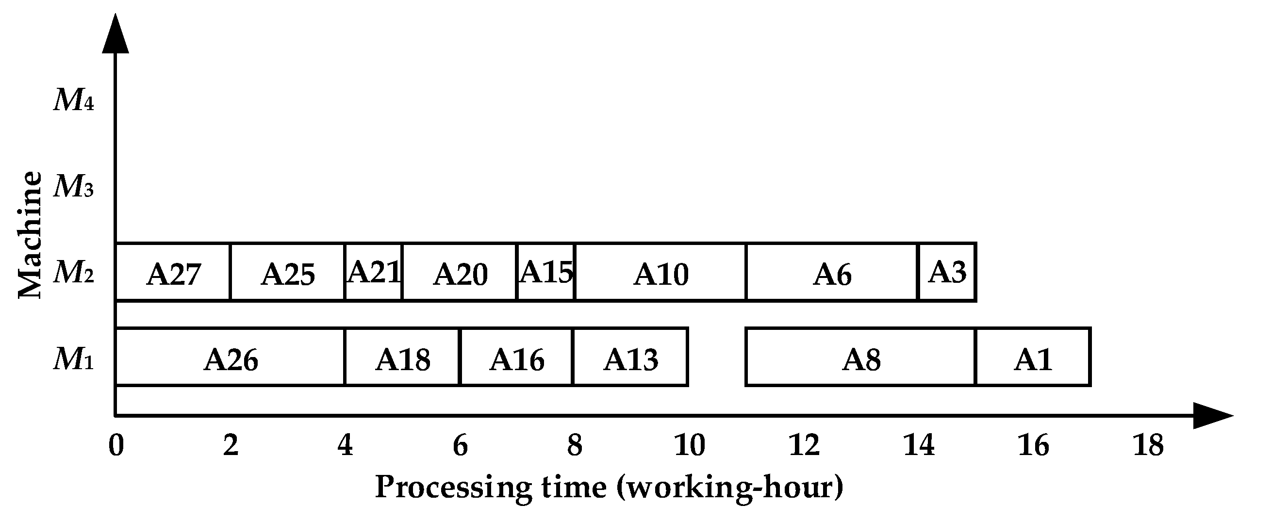
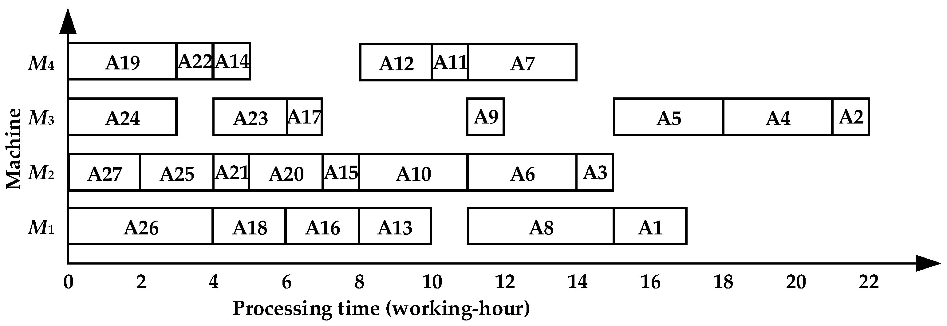
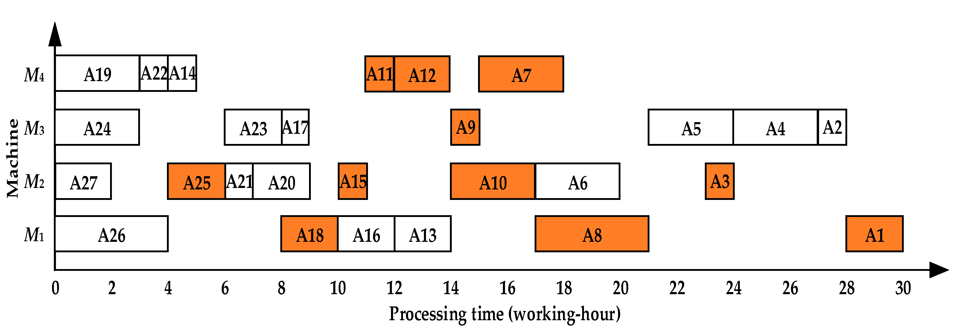
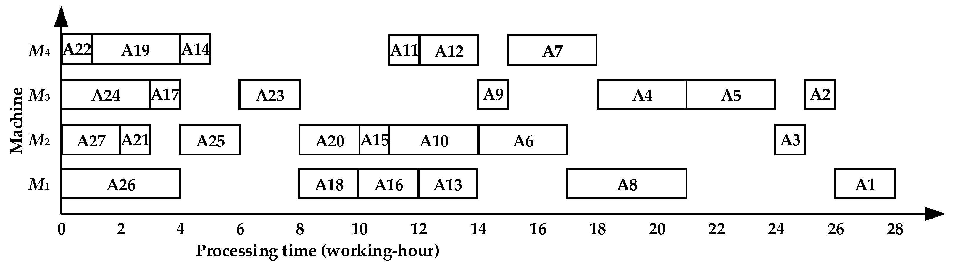
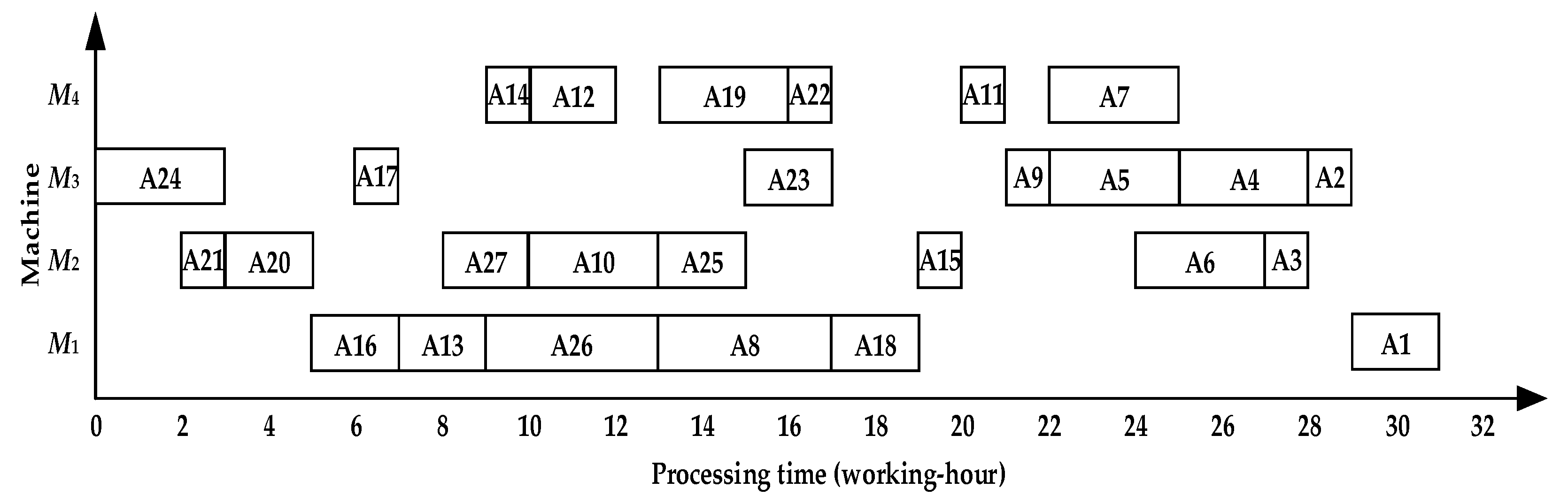
ANCOG is adopted to prioritize operation scheduling in the closely connecting operation groups, which ignores the influence of the relative position of operations with a low constraint degree on the scheduling results and leads to the idle time periods in the operations during the serial scheduling process. A comparative analysis of Figure 8 and Figure 9 shows that the multi-operation machine M₂ in Figure 9 has a long idle time from t = 17 to t = 24 with a total of 10 working hours. Due to the priority scheduling of A20 of the special machine M₂, in Figure 8, A16, A12, A9, A7, and A4, are 5, 4, 2, 2, and 4 working hours ahead of those in Figure 9.

(2)

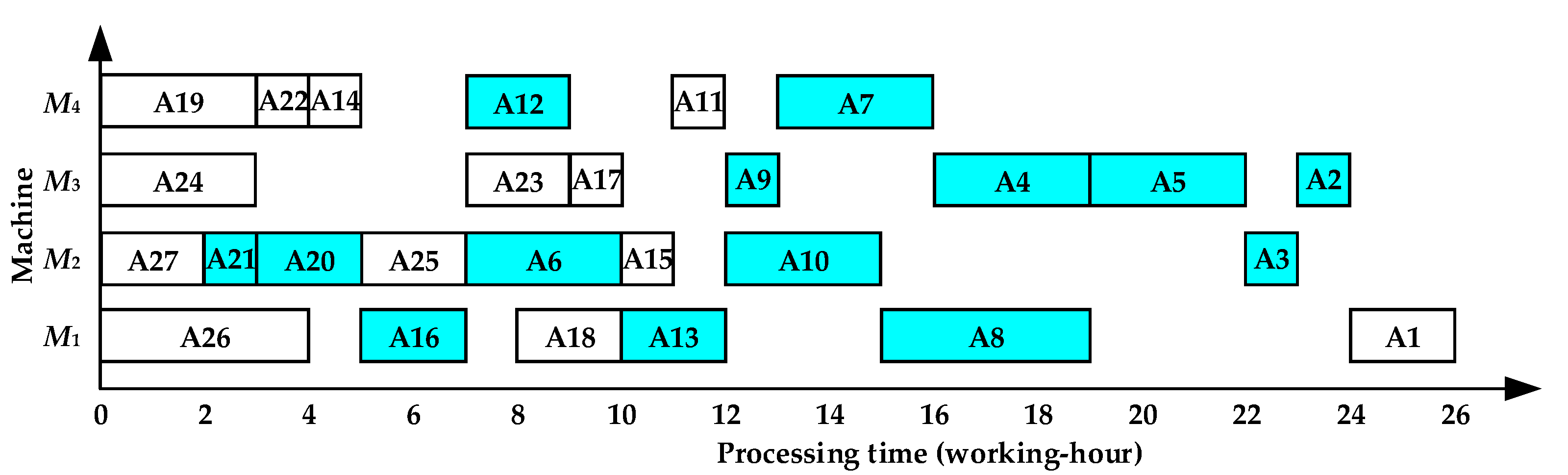
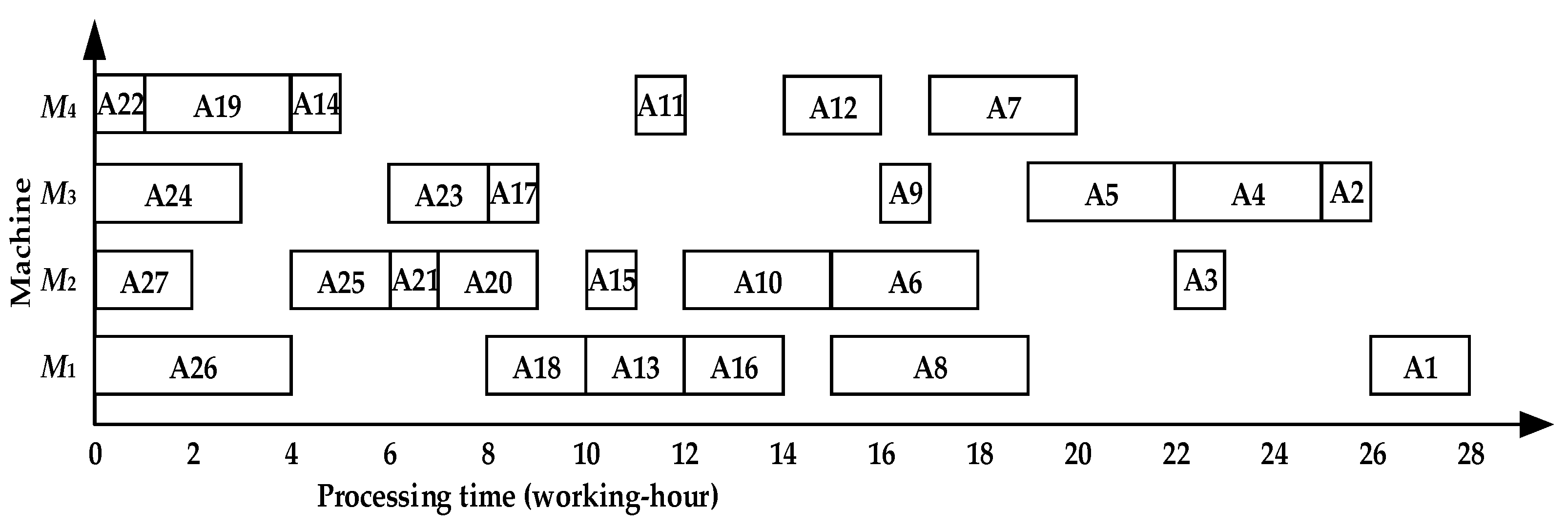
TSACCSP does not consider the processing and utilization of multi-operation machines during the determination of the starting time of operations, which affects the overall scheduling effect. A comparative analysis of Figure 8 and Figure 10 shows that the more-time machine M₂ is idle from t = 0 to t = 2, t = 5 to t = 7, t = 14 to t = 18, and t = 19 to t = 24 in Figure 10. In Figure 8, the starting times of A27, A25, A15, A6, and A3 are 7, 8, 17, and 5 working hours, earlier than those in Figure 10, respectively. This only increases the tightness of continuous processing on M₂, but it also increases the more-time machine utilization rate by 9.9%.

(3)

In ACHSO, the focus of optimization is operations at the same layer. The strategies of “Layer first” and “Leaf node process of the same layer first” are both horizontal optimization in nature, and the problem of “emphasizing the horizontal while neglecting the vertical” appears. A comparative analysis of Figure 8 and Figure 11 shows that, due to the priority scheduling of process A21 in Figure 8, its subsequent operations {A16, A12, A9, A7, A4} are 7, 7, 4, 4, and 6 working hours earlier than those shown in Figure 11. This realizes the close processing of the operations.

(4)

In HIS-PCVM, the multi-operation machines and the more-time machines are added to the integrated scheduling mechanism as special factors. First, the layer priority strategy and leaf node operation priority strategy ensure the parallel processing effect of the special machine. Then, for the general machine, according to the scheduling principles of the path value and the constraint degree from large to small, the subsequent operations of the operations on special equipment can be processed as soon as possible, vertically.

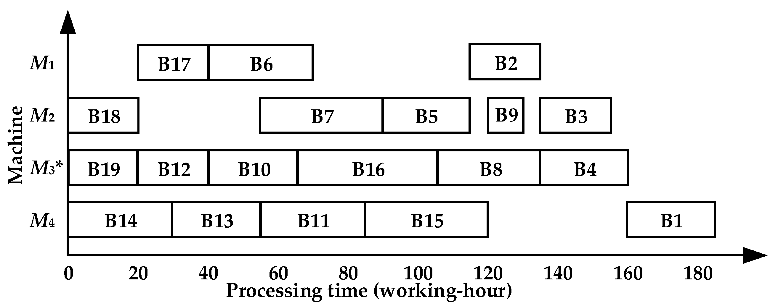
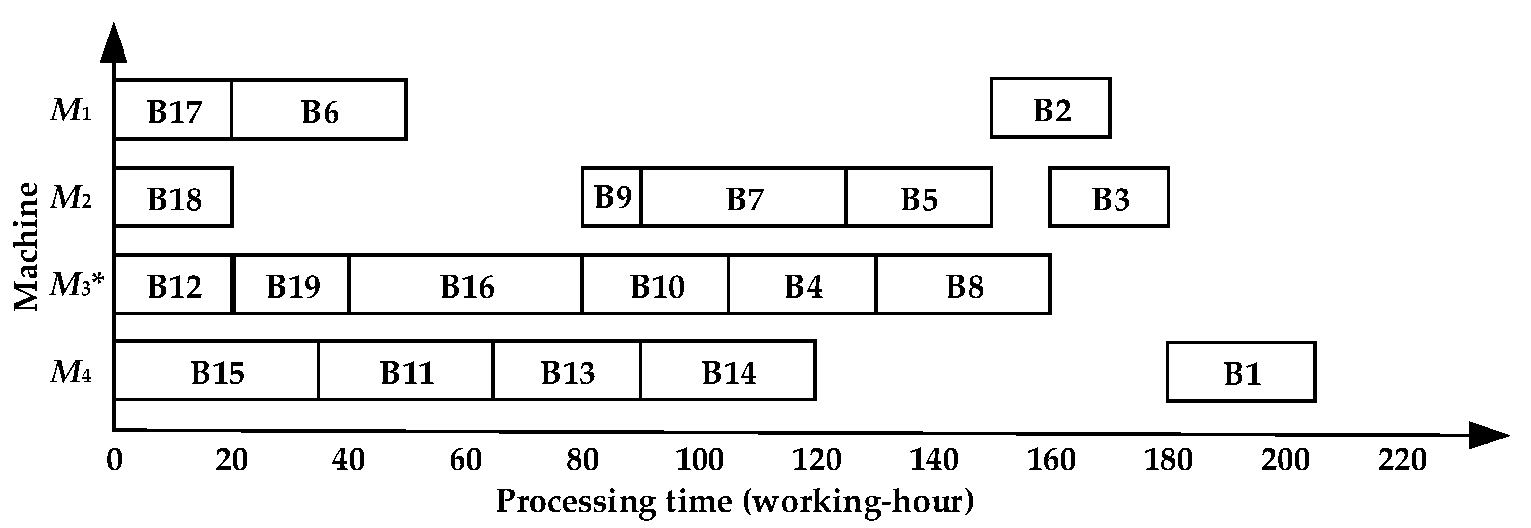
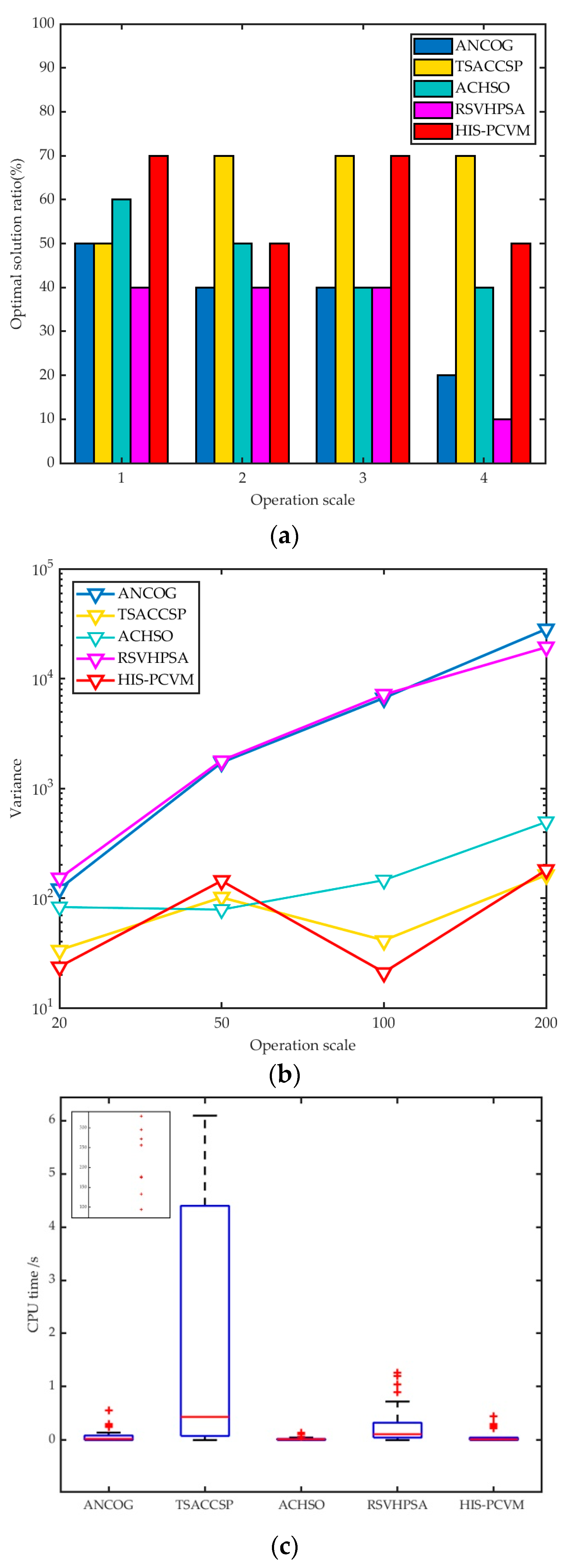
4.3. Comparison and Analysis of Symmetric Complex Product Scheduling

Assume symmetric complex product B, as shown in Figure 12, has 19 operations to be processed on four machines. For symmetric complex product B, the special equipment is unique, that is, M₃. It is not only a multi-operation machine but also a more-time machine. The general machines are M₁, M₂, and M₄.

The scheduling sequence by HIS-PCVM on M₃ is {B19, B13, B11, B6, B9, B4}, and on the general machine, it is {B18, B15, B14, B12, B17, B8, B7, B16, B5, B3, B2, B10, B1}, as shown in Figure 13. The makespan is 185 working hours.

Refs. [34,35,36,37,38,39,40] are all studies on the integrated scheduling problem with machine as the research object. As the latest algorithm, the algorithm (RSVHPSA) in Ref. [37] is selected to be compared and analyzed with the proposed algorithm. The experimental results also show the superiority of HIS-PCVM.

For the process tree of symmetric complex product B, the Gantt chart obtained by RSVHPSA is shown in Figure 14, and the total processing time is 205 working hours.

According to the symmetric complex product B, the makespan of the product by HIS-PCVM is 185 working hours, and by RSVHPSA, it is 205 working hours. The comparison and analysis of the two algorithms’ scheduling results are shown in

Table 3. Comparison and analysis of scheduling results of two algorithms of symmetric complex product B.

	HIS-PCVM	RSVHPSA
Algorithm idea	1. On the special machine: using the strategies of “the layer priority”, “the leaf node operation first”, and “the long processing time first” to establish the scheduling sequence; 2. On the general machine: using the strategies of “the highest path value priority”, “the layer priority”, and “the highest constraint degree priority” to establish the scheduling sequence.	1. Split symmetric process tree into several sub-trees; 2. Establish the pre-scheduling sequence according to the descending order of processing time of sub-trees; 3. On the same machine: establish the scheduling sequence by the machine process pre-start time.
Schedule sequence	{B19, B16, B10, B12, B8, B4, B18, B13, B11, B17, B6, B5, B15, B14, B3, B2, B9, B1}	M1: {B17, B6, B2}; M2: {B18, B7, B5, B9, B3}; M3: {B12, B19, B16, B10, B4, B8}; M4: {B15, B11, B13, B14}.
Total processing time	185	205
Overall utilization rate of machine	75.4%	67.8%

.

HIS-PCVM and RSVHPSA have the same characteristics, that is, they focus on the “machine” as the optimization object. However, HIS-PCVM is better than RSVHPSA. The reason is as follows.

RSVHPSA only considers the operations and ignores the variety of the machines. It leads to insufficient consideration of the competitive resources of the relatively tight machine on the scheduling effect. Comparing Figure 13 and Figure 14, on special equipment in Figure 13, B19 starts to be scheduled at time t = 0. This is 20 working hours earlier than the scheduling time in Figure 14. This greatly shortens the makespan of product B. As shown in Table 3, the relative improvement ratio of machine overall utilization obtained by HIS-PCVM is 7.6% higher than that obtained by RSVHPSA.

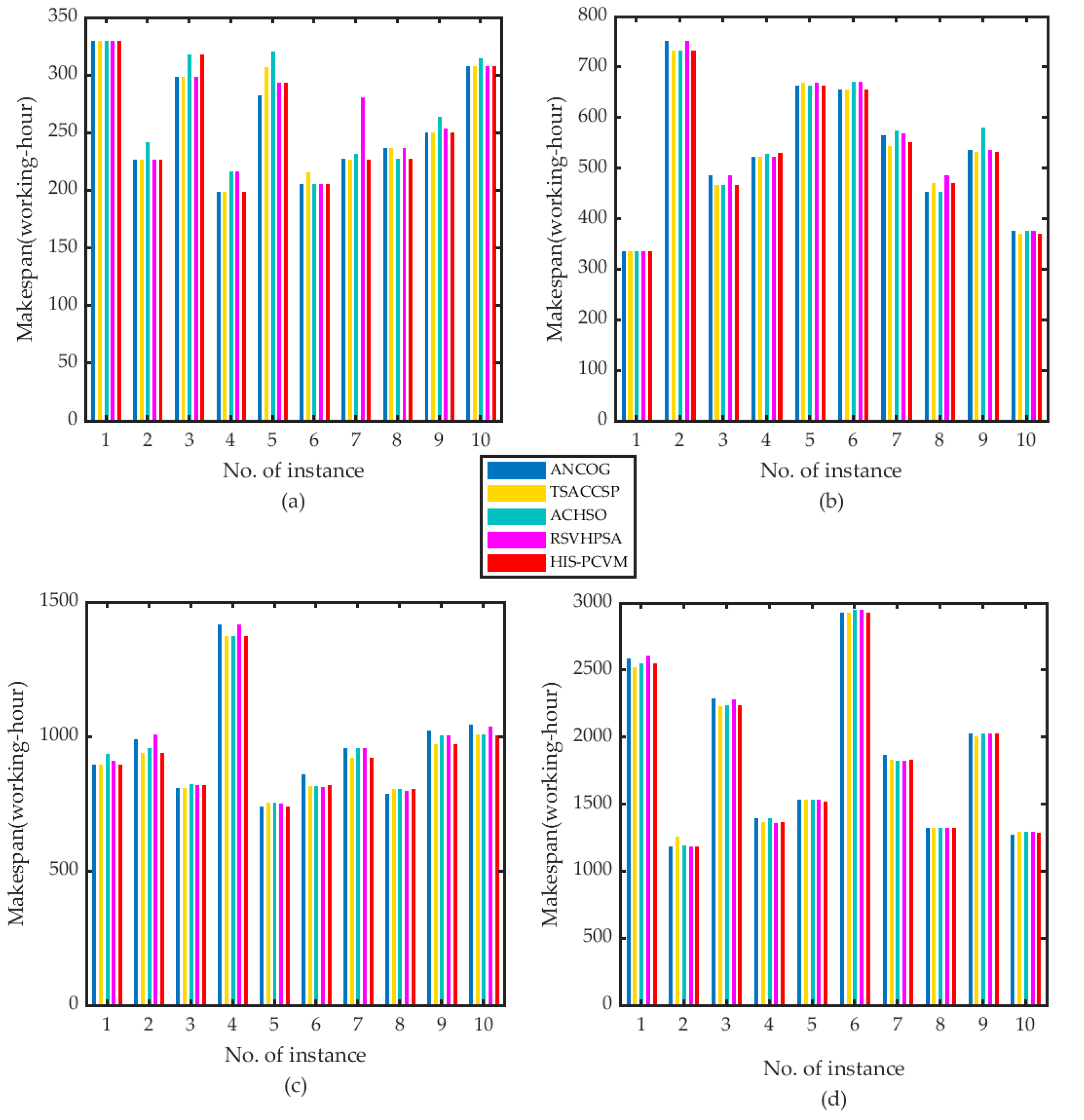
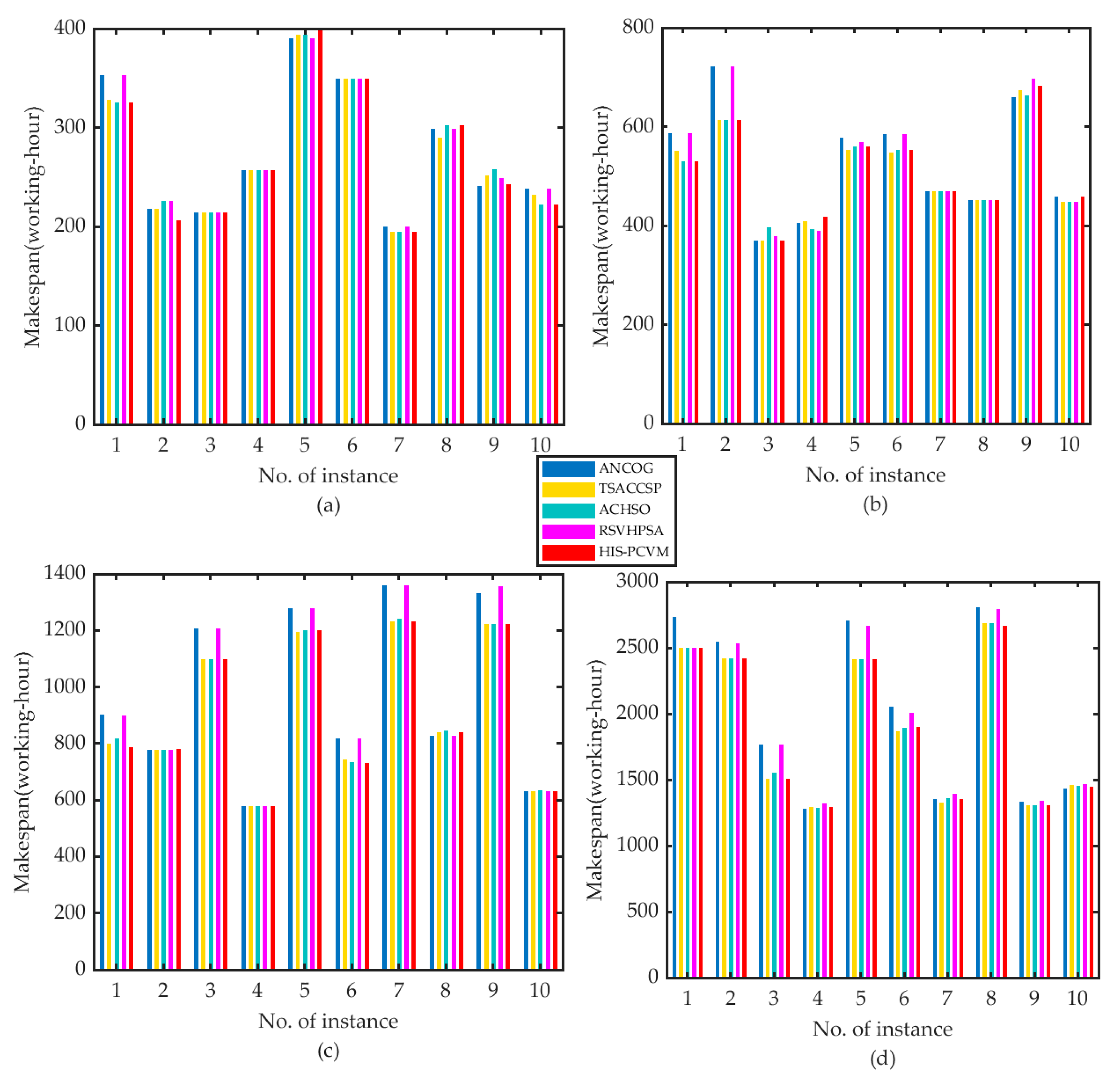
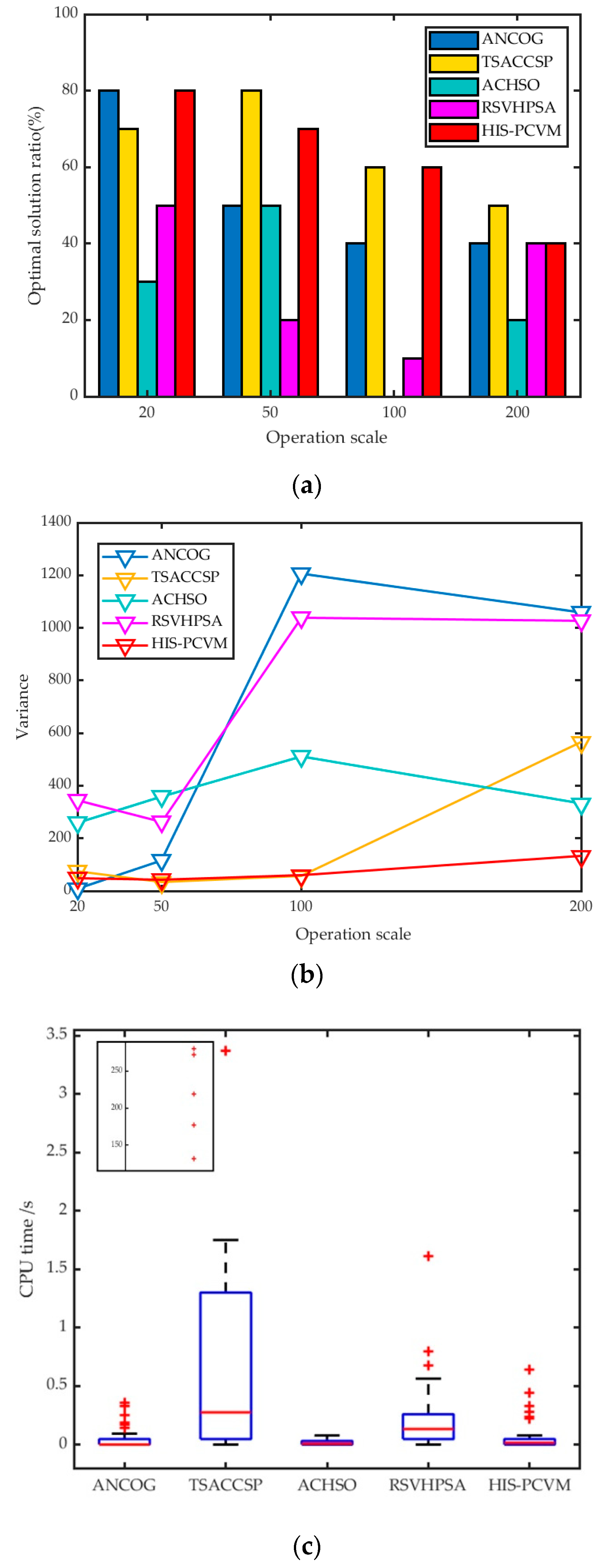
4.4. Comparison and Analysis of Five Scheduling Algorithms

In order to verify the effectiveness of HIS-PCVM and its adaptability to complex products with symmetric or asymmetric structures, this paper randomly selects 80 instances with four operation scales on five machines. The instances can be divided into two groups according to their structures, that is, the symmetric and the asymmetric structure. Each group has four operation scales, that is, [20, 50, 100, 200]. Each scale has ten different instances. As the number of machines is five, the average operations on each machine are [4, 10, 20, 40], which is in an ascending order. All the product instances are scheduled by the ANCOG, TSACCSP, ACHSO, RSVHPSA, and HIS-PCVM, respectively. They are all implemented on Matlab 2019 on the same PC. The makespans of the 80 instances by five algorithms are given in Figure 15 and Figure 16. To be more intuitive in comparing the five algorithms, the optimal solution ratio, the variance curves, and CPU time are all given in Figure 17 and Figure 18.

For products with asymmetric structures, in Figure 17a, we can see that the optimal solution ratios of all the algorithms are descending when the operation scale increases. The results of TSACCSP seem to be the best, which always keeps a high rate in each operation scale. The results of HIS-PCVM are better than the other three algorithms, and the effectiveness of it wanes when the scale is too large. However, when we see it in conjunction with Figure 17b,c, the performance of HIS-PCVM is the best. The variance curve of HIS-PCVM is always at a low level, and it is more stable than the other four algorithms. This means that although the optimal solution ratio of HIS-PCVM is not high, the obtained solutions can be closer to the best one. The CPU time of HIS-PCVM is better than TSACCSP. TSACCSP needs to compare all the available time points of all the operations, so it will spend more time when the scale is large. The CPU time of ACHSO is the best, but the performance is also the worst.

Figure 18 shows the results of products with symmetric structures. In Figure 18a, the optimal solution ratios of TSACCSP always keep a relatively high rate in large operation scales. Although the optimal solution ratio of HIS-PCVM is slightly less than TSACCSP, it also has a good performance. However, when we see it in conjunction with Figure 18b,c, it is better to choose HIS-PCVM rather than TSACCSP. This is because the variance curve of HIS-PCVM is at a lower level than TSACCSP, and the CPU time of HIS-PCVM is better than TSACCSP. Just like the results of asymmetric structures, TSACCSP needs to spend more time when the operation scale is large. Additionally, the performances of the other three algorithms are poor, although the CPU time of ACHSO is the best.

Therefore, the scheduling effect of HIS-PCVM is better, and it is a wise choice to adopt this algorithm for both products with symmetric and asymmetric structures. The main advantages are as follows:

(1)

HIS-PCVM adopts the optimization strategy of “special equipment”. It takes the particularity of machine resources as the research perspective. Additionally, it internalizes the overall optimization effect of integrated scheduling into the optimization of special equipment, so as to drive further optimization of the other machines.

(2)

The strategies of “the layer priority” and “the path value” fully compensate for the disadvantages of “attaching importance to horizontal optimization and discarding vertical optimization“ and “attaching importance to vertical optimization and discarding horizontal optimization“ in integrated scheduling. HIS-PCVM not only considers the leaf node operations with low layer priority but also considers the scheduling problem on the long path.

(3)

HIS-PCVM adopts the strategy of “the earliest scheduling time”, which effectively uses the scheduling gap between the serial operations caused by inserting the relevant operations into the idle time of the machine.

(4)

HIS-PCVM adopts the strategy of “the constraint degree”, which is based on the structure properties of the product itself, to comprehensively consider the various constraint relations between the processing operations. It solves the problem of processing gaps on machines due to a weak tight cohesion between the operations.

5. Conclusions and Future Research

In this work, an integrated scheduling algorithm considering special equipment processing characteristics is proposed to optimize the scheduling results and shorten the production time of both symmetric and asymmetric complex products. The conclusions are drawn as follows:

(1)

This paper takes “the special equipment processing characteristics” as the important optimization factors. It considers the variety of machine processing characteristics and the influence of complex products on scheduling results. It achieves the effect of optimizing integrated scheduling by scheduling the operations corresponding to the special equipment.

(2)

The proposed algorithm realizes both horizontal optimization and vertical optimization by the layer priority strategy, the earliest scheduling time strategy, and the path value strategy. The layer priority strategy realizes parallel optimization in landscape orientation. The other two strategies realize optimization in the longitudinal direction.

(3)

It reduces the serial gap between operations, improves machine utilization, and shortens the makespan of complex products. Thus, it provides a new method to solve the integrated scheduling problem and expands the ideas on solving the problem. Therefore, the proposed algorithm has a certain theoretical and practical significance.

Next, the following research directions are suggested. Firstly, more optimization algorithms can be introduced to enhance the ability to solve integrated scheduling problems. Secondly, the integrated scheduling problems with special constraints need to be considered, such as a flexible production environment. Furthermore, the multi-objective integrated scheduling problem is also one of the future research directions.

References

1. Xu, G.; Chen, Y. Petri-net-based scheduling of flexible manufacturing systems using an estimate function. Symmetry 2022, 14, 1052. [Google Scholar] [CrossRef]
2. Yang, Y.; Wang, Z.; Hu, Z.; Yang, Y. Research on optimal scheduling strategy for multi-energy interconnection. In China Intelligent Automation Conference; Springer: Singapore, 2021; pp. 185–197. [Google Scholar]
3. Li, M.; Xiong, H.; Lei, D. An artificial bee colony with adaptive competition for the unrelated parallel machine scheduling problem with additional resources and maintenance. Symmetry 2022, 14, 1380. [Google Scholar] [CrossRef]
4. Tang, Y.; Pan, Z.; Pedrycz, W.; Ren, F.; Song, X. Viewpoint-based kernel fuzzy clustering with weight information granules. In Proceedings of the IEEE Transactions on Emerging Topics in Computational Intelligence, Piscataway, NJ, USA, 2 September 2022. [Google Scholar] [CrossRef]
5. Tang, Y.; Ren, F.; Pedrycz, W. Fuzzy c-means clustering through SSIM and patch for image segmentation. Appl. Soft Comput. 2020, 87, 105928. [Google Scholar] [CrossRef]
6. Ibrahim, A.M.; Tawhid, M.A. An improved artificial algae algorithm integrated with differential evolution for job-shop scheduling problem. J. Intell. Manuf. 2022, 1–16. [Google Scholar] [CrossRef]
7. Wu, K.; Dai, A.; Zheng, X.; Xi, W.; Shun, F. Economically optimized scheduling of cogeneration micro-grid considering pollution emission cost. In Proceedings of the China Process Control Conference, Taiyuan, China, 30 July 2021. [Google Scholar] [CrossRef]
8. Xia, Y.; Xie, Z.; Xin, Y.; Zhang, X. A multi-shop integrated scheduling algorithm with fixed output constraint. J. Intell. Fuzzy Syst. 2021, 41, 4609–4617. [Google Scholar] [CrossRef]
9. Samee, N.M.A.; Ahmed, S.; Abul, S. Metaheuristic algorithms for independent task scheduling in symmetric and asymmetric cloud computing environment. J. Comput. Sci. 2019, 15, 594–611. [Google Scholar] [CrossRef] [Green Version]
10. Hidri, L.; Elsherbeeny, A.M. Optimal Solution to the two-stage hybrid flow shop scheduling problem with removal and transportation times. Symmetry 2022, 14, 1424. [Google Scholar] [CrossRef]
11. Mao, L.; Guo, W. Research on collaborative planning and symmetric scheduling for parallel shipbuilding projects in the open distributed manufacturing environment. Symmetry 2020, 12, 161. [Google Scholar] [CrossRef]
12. Vincent, T.; Lei, S.; Federico, D. Exponential time algorithms for just-in-time scheduling problems with common due date and symmetric weights. J. Comb. Optim. 2020, 39, 764–775. [Google Scholar]
13. Zhang, F.; Bai, J.; Yang, D.; Wang, Q. Digital twin data-driven proactive job-shop scheduling strategy towards asymmetric manufacturing execution decision. Sci. Rep. 2022, 12, 1546. [Google Scholar] [CrossRef] [PubMed]
14. Fabry, Q.; Agnetis, A.; Berghman, L.; Briand, C. Complexity of flow time minimization in a crossdock truck scheduling problem with asymmetric handover relations. Oper. Res. Lett. 2022, 50, 50–56. [Google Scholar] [CrossRef]
15. Nanthini, S.; Nithya, K.; Sudhakar, S. Dominating set based virtual backbone cluster scheduling for ensuring energy efficiency in asymmetric radio WSN. J. Ambient. Intell. Humaniz. Comput. 2021, 13, 4569. [Google Scholar]
16. Yonghee, Y.; Eun, J.; Young, H. Adaptive genetic algorithm for energy-efficient task scheduling on asymmetric multiprocessor system-on-chip. Microprocess. Microsyst. 2019, 66, 19–30. [Google Scholar]
17. Wang, Q.; Chen, G. Robust control for asymmetric saturated systems based on gain scheduling. In Proceedings of the 29th China Control and Decision Making Conference, Chongqing, China, 28–30 May 2017. [Google Scholar]
18. Xie, Z. Study on Operation Scheduling of Complex Product with Constraint among Jobs. Ph.D. Thesis, Harbin University of Science and Technology, Harbin, China, 2009. [Google Scholar]
19. Xie, Z.; Yang, D.; Ma, M.; Yu, X. An improved artificial bee colony algorithm for the flexible integrated scheduling problem using networked machines collaboration. Int. J. Coop. Inf. Syst. 2020, 29, 2040003–2040022. [Google Scholar] [CrossRef]
20. Gao, Y.; Xie, Z.; Liu, X.; Zhou, W.; Yu, X. Integrated scheduling algorithm based on the priority constraint table for complex products with tree structure. Adv. Mech. Eng. 2020, 12, 1687814020985206. [Google Scholar] [CrossRef]
21. Defersha, F.; Obimuyiwa, D.; Yimer, A. Mathematical model and simulated annealing algorithm for setup operator constrained flexible job shop scheduling problem. Comput. Ind. Eng. 2022, 171, 108487–108509. [Google Scholar] [CrossRef]
22. Hou, L.; Tian, E.; Zhou, Y.; Lu, P.; Wang, T.; Zhang, Y.; Liu, Z.; Yang, Y.; Li, P. Robust optimization of multiple microgrids scheduling for integrated energy system with uncertain sources and loads. In Proceedings of the 2020 International Conference on Green Energy, Environment and Sustainable Development (GEESD), Wuhan, China, 24–25 April 2020. [Google Scholar]
23. Chen, J.; Du, W.; Wang, H.; Guo, D. Research on integrated scheduling optimization of double-trolley quay crane and AGV in automated terminal. In Proceedings of the 2019 2nd International Conference on Communication, Network and Artificial Intelligence (CNAI), Guangzhou, China, 27–29 December 2019. [Google Scholar]
24. Sun, F.; Cao, J.; Lu, Z. HEFT-dynamic scheduling algorithm in workflow scheduling. In Proceedings of the 34th China Control and Decision Making Conference, Hefei, China, 21–23 May 2022. [Google Scholar]
25. Yu, M.; Wang, Y.; Lv, Y.; Zhou, Y. Research on cooperative scheduling of yard crane and external container truck based on hybrid genetic algorithm and grey wolf optimization. In Proceedings of the 2022 World Transport Conference (WTC), Copenhagen, Denmark, 2–8 September 2022. [Google Scholar]
26. Xie, Z.; Teng, Y.; Yang, J. Integrated scheduling algorithm with no-wait constraint operation group. Acta Autom. Sin. 2011, 122, 371–379. [Google Scholar] [CrossRef]
27. Xie, Z.; Zhang, X.; Gao, Y.; Xin, Y. Time selective integrated scheduling algorithm considering the compactness of serial processes. J. Mech. Eng. 2018, 54, 191–202. [Google Scholar] [CrossRef]
28. Xie, Z.; Zhou, W.; Yang, J. Resource cooperative integrated scheduling algorithm considering hierarchical scheduling order. Comput. Integr. Manuf. Syst. 2022, 1–17. Available online: http://kns.cnki.net/kcms/detail/11.5946.TP.20220104.1623.002.html (accessed on 7 September 2022).
29. Papatya, S.; Tusan, D.; İmdat, K. Solution approaches for the parallel machine order acceptance and scheduling problem with sequence-dependent setup times, release dates and deadlines. Eur. J. Ind. Eng. 2021, 15, 295–318. [Google Scholar]
30. Xie, Z.; Xin, Y.; Yang, J. Machine-driven integrated scheduling algorithm with rollback-preemptive. Autom. Sin. 2011, 37, 1332–1343. [Google Scholar]
31. Xie, Z.; Li, S.; Liu, S. A scheduling algorithm based on key machine compact procedures. J. Harbin Univ. Technol. 2003, 37, 41–45. [Google Scholar]
32. Xie, Z.; Zheng, Q.; Liu, S. A dynamic scheduling algorithm based on key machine’s compact procedures. J. Harbin Univ. Technol. 2003, 50–53. [Google Scholar] [CrossRef]
33. Xie, Z.; Yang, G.; Tan, G. An algorithm of JSSP with dynamic collection of job with priority. Inst. Eng. Technol. Chin. Mech. Eng. Soc. 2006, 11, 398–402. [Google Scholar] [CrossRef]
34. Zhang, H. Hybrid Gs-Ga algorithm for parallel machine scheduling problem with different transport vehicles. In Proceedings of the 2021 International Conference on Applied Mathematics, Modeling and Computer Simulation (AMMCS), Wuhan, China, 13–14 November 2021. [Google Scholar]
35. Luo, C.; Geng, Z. Single machine scheduling problem with controllable setup and job processing times and position-dependent workloads. In Proceedings of the 2019 2nd International Conference on Communication, Network and Artificial Intelligence (CNAI), Guangzhou, China, 27–29 December 2019. [Google Scholar]
36. Zheng, Y.; Xiao, Y. A mathematical formulation for integrated scheduling problem of handling equipment in container terminals. In Proceedings of the 2nd International Conference on Economics and Management, Education, Humanities and Social Sciences (EMEHSS), Wuhan, China, 29–30 March 2018. [Google Scholar]
37. Xie, Z.; Teng, H. Anak Agung Ayu Putri Ardyanti1. An integrated scheduling algorithm for the same equipment process sequencing based on the root-subtree vertical and horizontal pre-scheduling. Comput. Model. Eng. Sci. 2022, 21550–21572. [Google Scholar] [CrossRef]
38. Jin, L.; Yu, X.; Dong, Z. Single-machine scheduling with piece-rate maintenance, interval constrained processing times and rejection penalties. In Proceedings of the 2018 3rd Joint International Information Technology, Mechanical and Electronic Engineering Conference (JIMEC), Chongqing, China, 15–16 December 2018. [Google Scholar]
39. Xu, B.; Zhang, Y.; Sun, K. Maintenance scheduling of power equipment considering opportunistic maintenance strategy. In Proceedings of the 2019 4th Asia Conference on Power and Electrical Engineering (ACPEE), Hangzhou, China, 28–31 March 2019. [Google Scholar]
40. Zhu, C.; Feng, S.; Zhang, C.; Jin, L.; Wang, L. Research on open shop scheduling problem considering equipment preventive maintenance. China Mech. Eng. 2022, 1–12. Available online: http://kns.cnki.net/kcms/detail/42.1294.th.20220810.1600.002.html (accessed on 7 September 2022).
Figure 1. Flow chart of the proposed algorithm framework.
Symmetry 14 02150 g001
Figure 2. Process tree of asymmetric complex product A.
Symmetry 14 02150 g002
Figure 3. Gantt chart of operations on the multi-operation machine.
Symmetry 14 02150 g003
Figure 4. Gantt chart of operations on the multi-operation machine and more-time machine.
Symmetry 14 02150 g004
Figure 5. New process tree of asymmetric complex product A after pruning.
Symmetry 14 02150 g005
Figure 6. Gantt chart of the initial scheduling of asymmetric complex product A.
Symmetry 14 02150 g006
Figure 7. Gantt chart of asymmetric complex product A after checking the constraint relationship.
Symmetry 14 02150 g007
Figure 8. Gantt chart of asymmetric complex product A after the adjustment at the earliest scheduling time of 26 working hours.
Symmetry 14 02150 g008
Figure 9. Gantt chart of asymmetric complex product A by ANCOG with 28 working hours.
Symmetry 14 02150 g009
Figure 10. Gantt chart of asymmetric complex product A in the reverse sequence by TSACCSP with 31 working hours.
Symmetry 14 02150 g010
Figure 11. Gantt chart of asymmetric complex product A by ACHSO with 28 working hours.
Symmetry 14 02150 g011
Figure 12. Process tree of symmetric complex product B.
Symmetry 14 02150 g012
Figure 13. Gantt chart of symmetric complex product B by HIS-PCVM with 185 working hours. (* Indicates the special equipment is unique.)
Symmetry 14 02150 g013
Figure 14. Gantt chart of symmetric complex product B by RSVHPSA with 205 working hours. (* Indicates the special equipment is unique).
Symmetry 14 02150 g014
Figure 15. Results of ANCOG, TSACCSP, ACHSO, RSVHPSA, and HIS-PCVM for integrated scheduling with asymmetric structures: (a) 20 operations, (b) 50 operations, (c) 100 operations, and (d) 200 operations.
Symmetry 14 02150 g015
Figure 16. Results of ANCOG, TSACCSP, ACHSO, RSVHPSA, and HIS-PCVM for integrated scheduling with symmetric structures: (a) 20 operations, (b) 50 operations, (c) 100 operations, and (d) 200 operations.
Symmetry 14 02150 g016
Figure 17. Comparison results of ANCOG, TSACCSP, ACHSO, RSVHPSA, and HIS-PCVM for integrated scheduling with asymmetric structures: (a) optimal solution ratio, (b) variance curves, and (c) CPU time (the points in the small square are the outliers for TSACCSP).
Symmetry 14 02150 g017
Figure 18. Comparison results of ANCOG, TSACCSP, ACHSO, RSVHPSA, and HIS-PCVM for integrated scheduling with symmetric structures: (a) optimal solution ratio, (b) variance curves, and (c) CPU time (the points in the small square are the outliers for TSACCSP).
Symmetry 14 02150 g018