
A Modification of the Imperialist Competitive Algorithm with Hybrid Methods for Multi-Objective Optimization Problems

Abstract
:1. Introduction
1.1. Description of Constrained Optimizaiton
1.2. Related Work
1.2.1. Multi-Objective Swarm and Evolutionary Algorithms
- (1)
- With the increase of the number of objective functions, the proportion of non-dominated solutions in the population also increases, which would lead to the slowing down in the speed of search process;
- (2)
- For high-dimensional target space, the computational complexity to maintain diversity is too high, and it is difficult to find the adjacent elements of the solution;
- (3)
- The indexes for evaluating comprehensive performance of the algorithm are poor. Almost all evaluation indexes can only evaluate one of the convergence and distribution of the population in the algorithm; therefore, it is presently difficult to comprehensively evaluate the population convergence and distribution of the swarm and evolutionary algorithms for solving multi-objective optimization;
- (4)
- For the high-dimensional target space, how to visualize the results is also a difficult problem.
1.2.2. Multi-Objective Imperialist Competitive Algorithms
1.3. The Main Content of This Paper
- (1)
- From the perspective of algorithm theory, this paper proposes a new scheme to solve multi-objective optimization problems based on HMICA. By calculating 12 multi-objective benchmarks and comparing with some high-quality algorithms in recent years, the algorithm proposed in this paper has certain advantages;
- (2)
- From the perspective of algorithm performance evaluation, this paper proposes a comprehensive evaluation method of multi-objective optimization algorithm by using multiple evaluation metrics.
2. The Proposed Algorithm
2.1. The Establishment of the Initial Empires
- (1)
- The feasible solution is better than the infeasible solution. If both solutions are infeasible solutions, compare the value of the violation function. The smaller the value of the violation function is, the better the solution is;
- (2)
- If both solutions are feasible solutions, first judge whether there is a dominant relationship between the two solutions. If one solution dominates the other, the dominant solution is the optimal solution and the dominated solution is the inferior solution;
- (3)
- If the two solutions are mutually non-dominated feasible solutions, arrange the number of dominated solutions of the two solutions in the whole population. The less the number of dominated solutions is, the better the solution is;
- (4)
- If the two solutions are mutually non-dominated feasible solutions, and the number of dominated solutions of the two solutions is the same in the whole population, the crowding distance is compared. The larger the crowding distance is, the better the solution is. The calculation process of the crowding distance can be seen in the literature [5].
2.2. Empire Competition
- (1)
- Comparing the number of infeasible solutions in each empire, where the empire with a smaller number is better;
- (2)
- If the number of infeasible solutions of the two empires is the same, compare the number of dominated solutions. The lower the number of dominated solutions, the better empire is;
- (3)
- If the above two are the same, compare the average crowding distance of each empire, where the larger the crowding distance is, the stronger empire is.
2.3. External Archive Strategy
2.4. Implementation of the Proposed Algorithm
| Algortithm 1: Pseudocode of MOHMICA | |
| Input: Population total number N The number of initial imperialists Nimp and colonies Ncol The number of optimization iterations MaxIt, archive size EA Output: MOHMICA Pareto front | |
| 1 | Initialize the MOHMICA population postions by Halton sequence |
| 2 | for i = 1: N do |
| 3 | Calculate the function values, violation values (if the optimization with constraints) the number of dominated solutions and crowding distance of the initial countries. |
| 4 | Sort initial solutions according to the sorting rules in the Section 2.1. |
| 5 | Create empires: according to the clonies allocating rules in the Section 2.1. |
| 6 | end for |
| 7 | while do |
| 8 | for i = 1:N do |
| 9 | The development of imperialists and the assimilation of colonies: according to literature [42]. |
| 10 | Calculate the function values, violation values (if the optimization with constraints) the number of dominated solutions and crowding distance of the initial countries. |
| 11 | Empire interaction: according to literature [42]. |
| 12 | Calculate the function values, violation values (if the optimization with constraints) the number of dominated solutions and crowding distance of the initial countries. |
| 13 | Empire revolution: according to literature [42]. |
| 14 | Calculate the function values, violation values (if the optimization with constraints) the number of dominated solutions and crowding distance of the initial countries. |
| 15 | Empire interaction: according to literature [42]. |
| 16 | Empire competition: according to the Section 2.2 of this paper. |
| 17 | Update external archive: according to the Section 2.3 of this paper. |
| 18 | end for |
3. Experimental Design
3.1. Benchmark Functions
3.2. Performance Metrics
- (1)
- Convergence metric
- (2)
- Diversity metric
- (3)
- Generational distance
- (4)
- Inverted generational distance
3.3. Comparison Algorithm and Simulation Setting
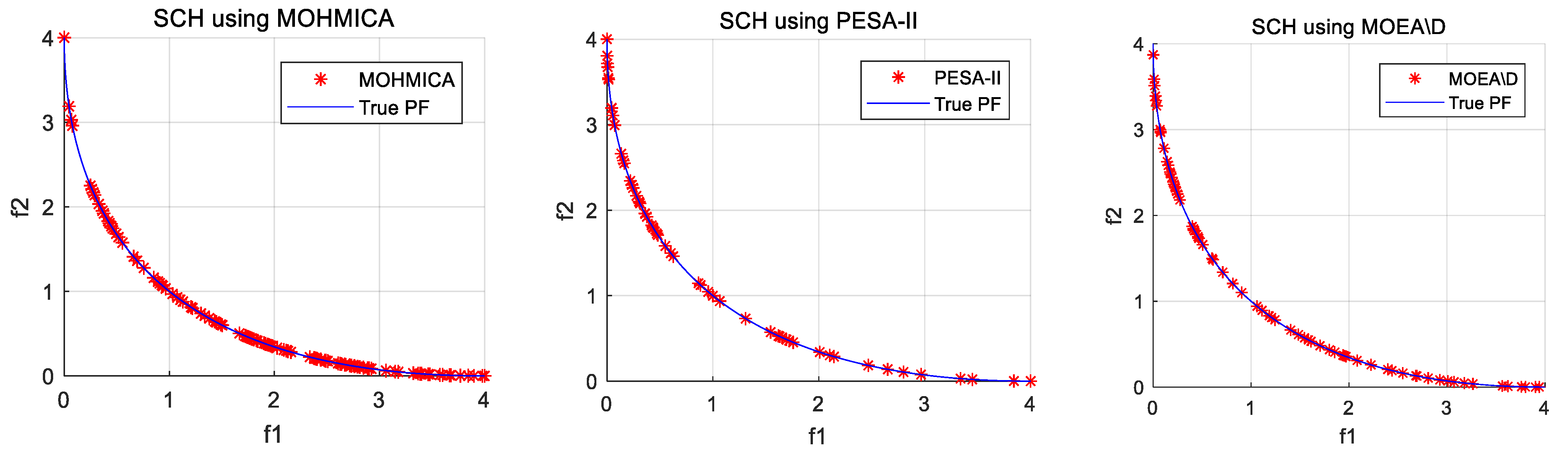
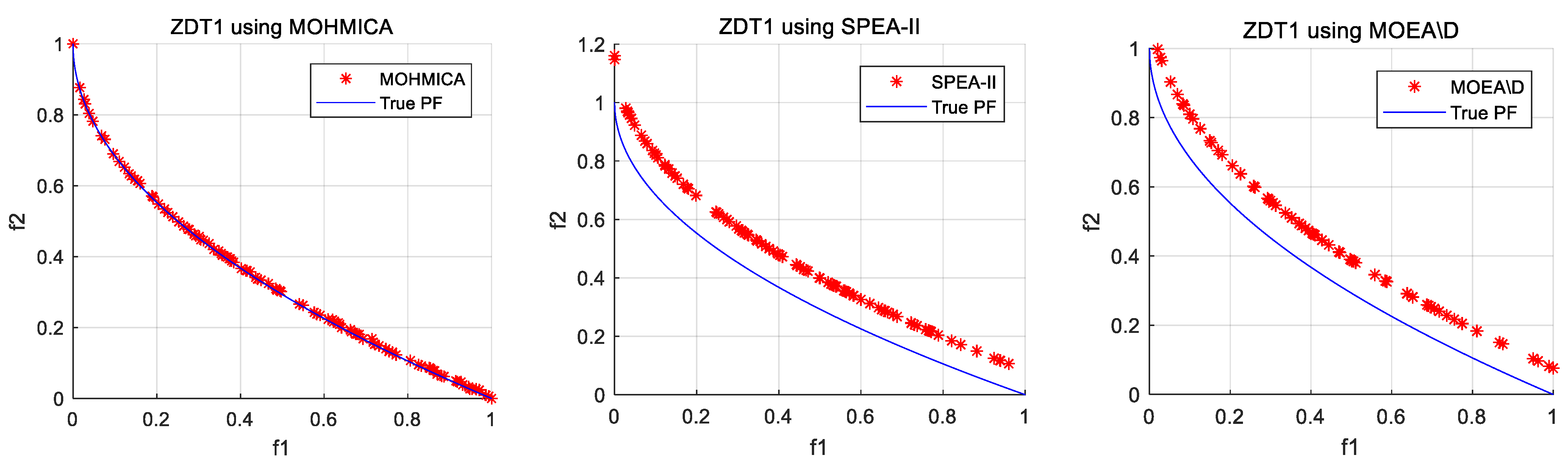
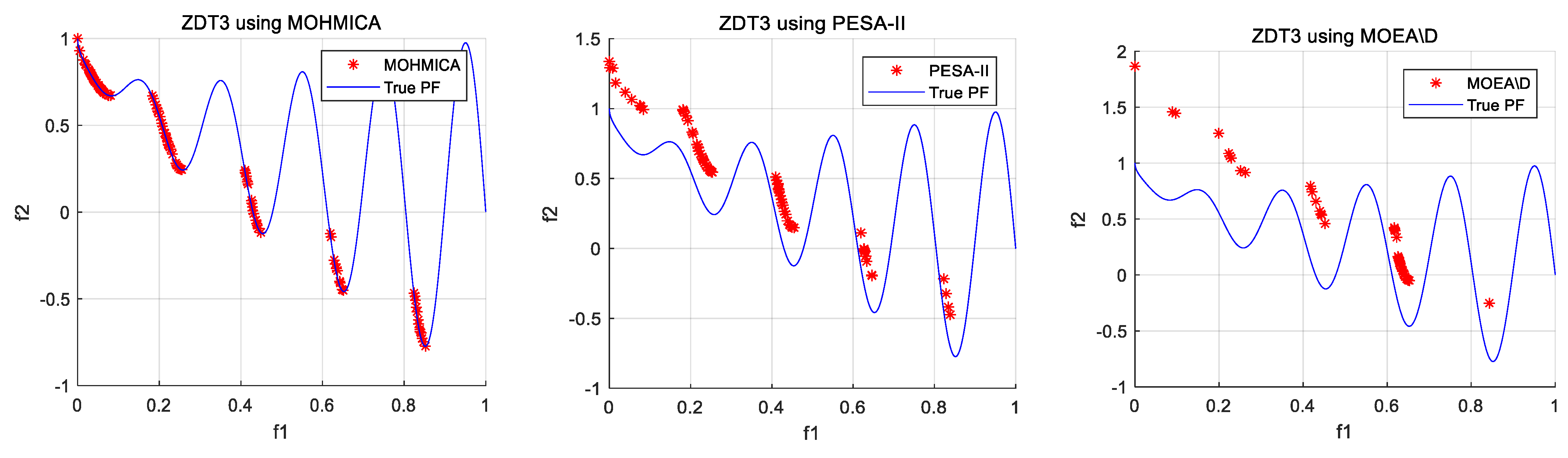
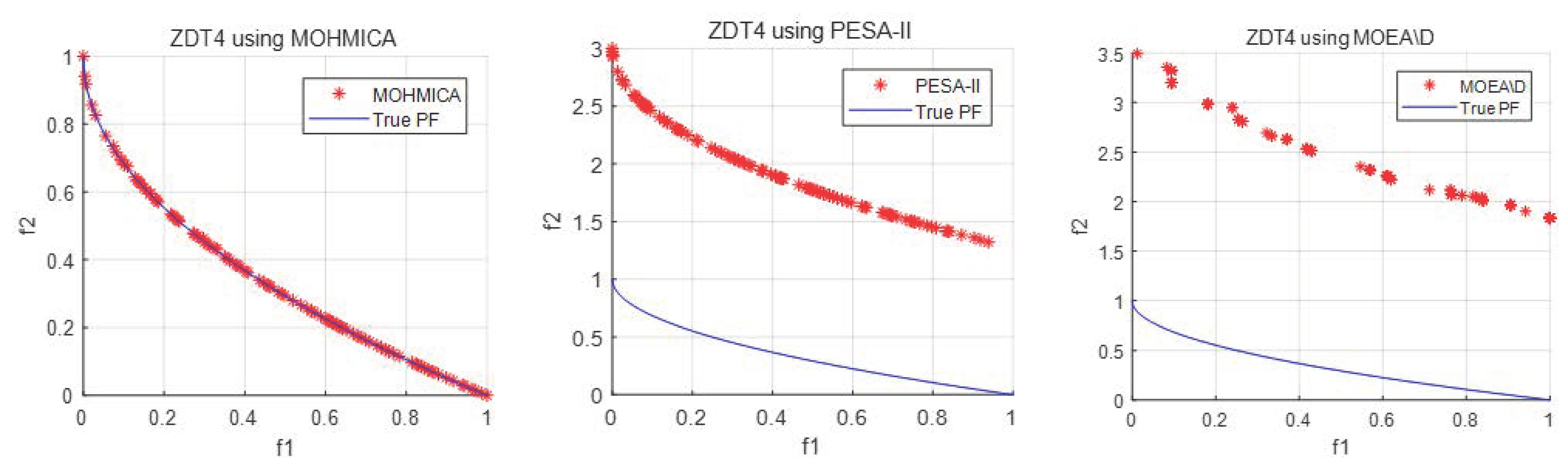
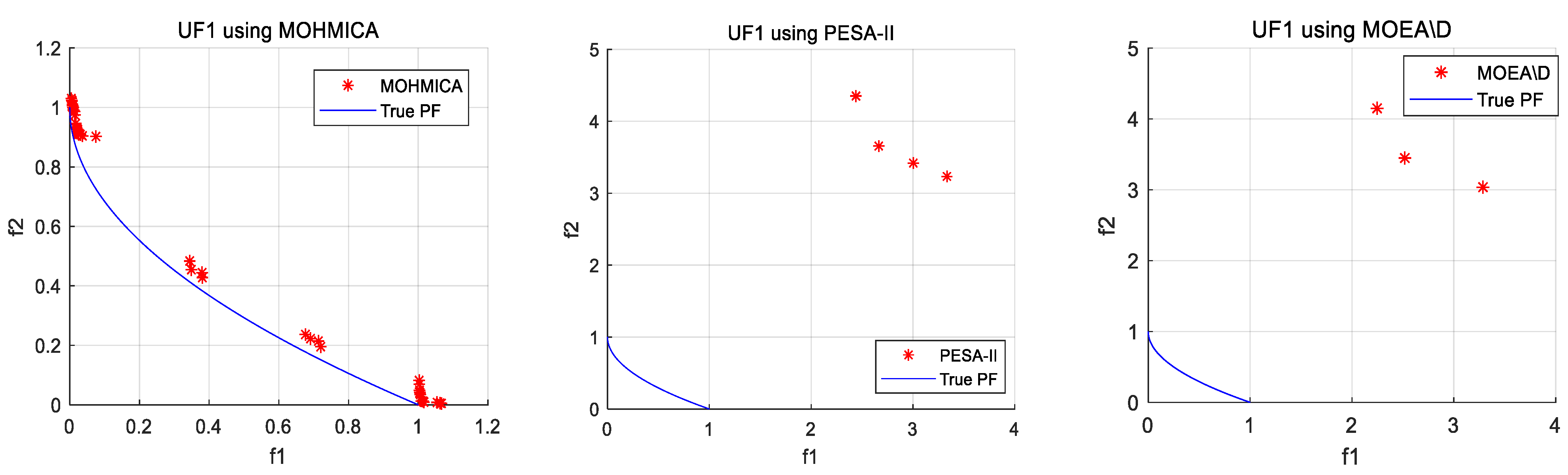
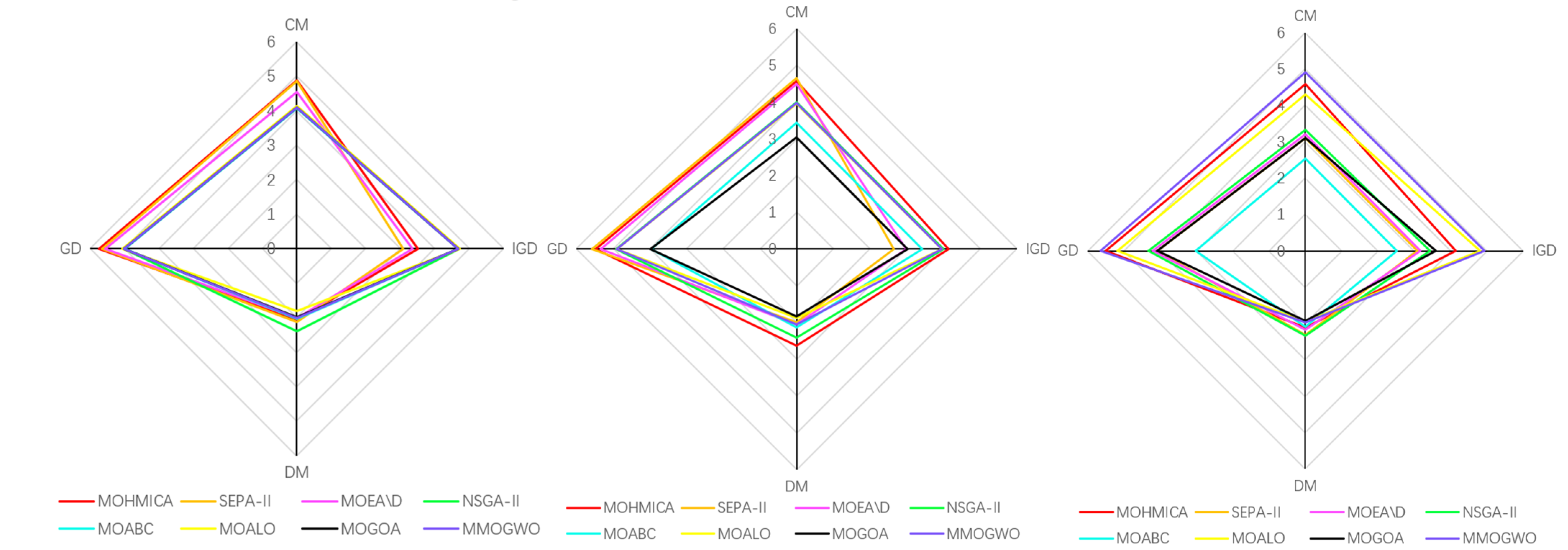
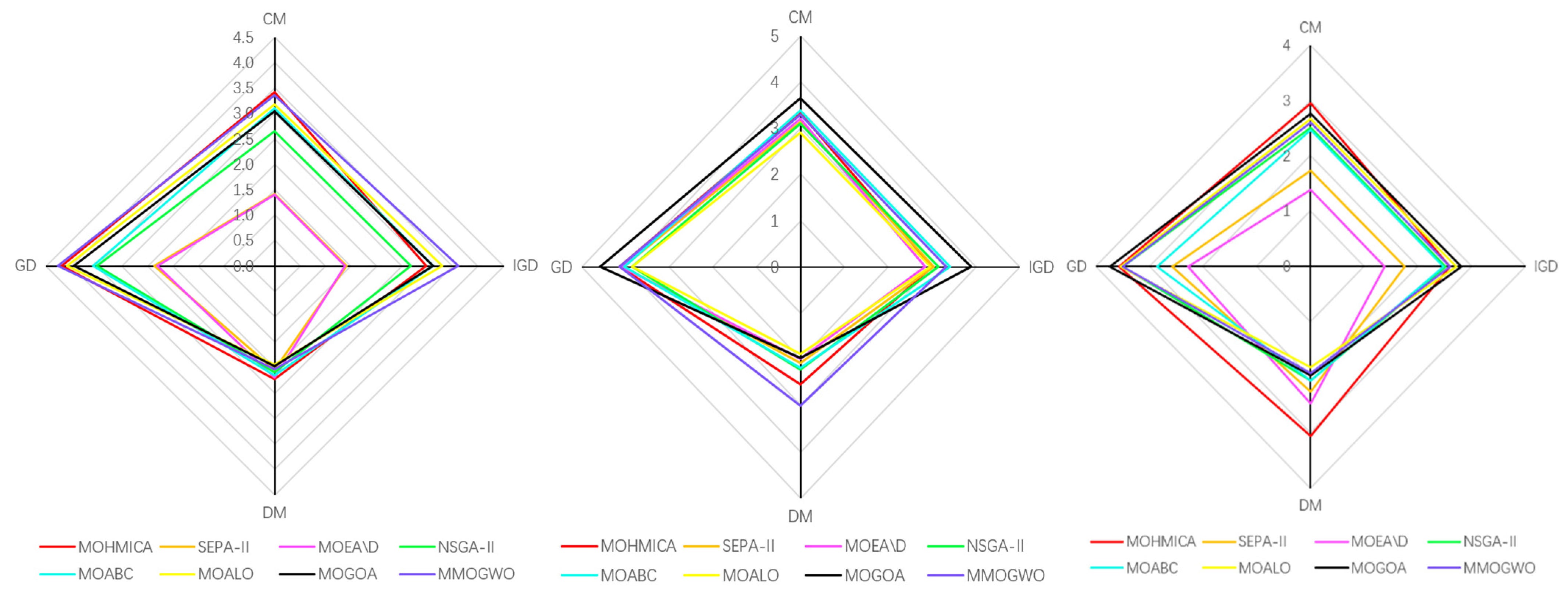
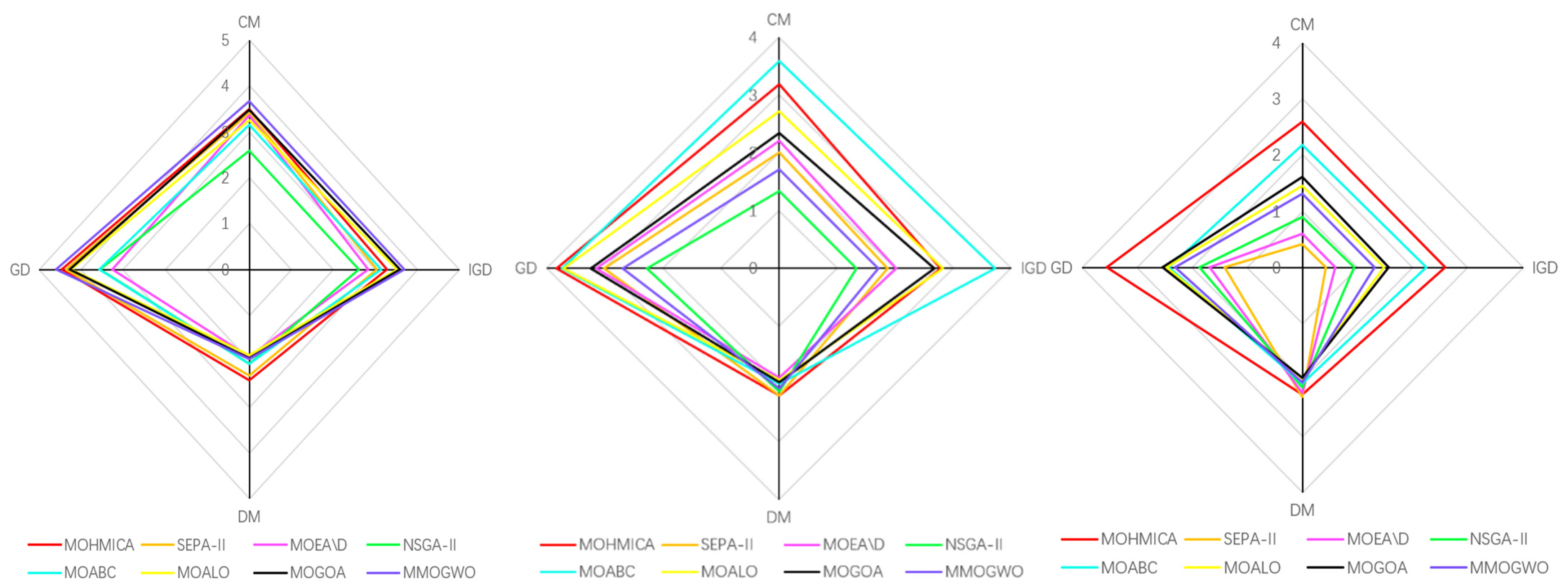
4. Results and Discussion
4.1. Calculation Results and Discussion of Benchmark Functions
- (1)
- H0: The results of the two algorithms are homogenous;
- (2)
- H1: The results of the two algorithms are heterogenous.
- (1)
- From the perspective of R+, MOHMICA has advantages over the other algorithms. Moreover, most of the results can pass the level of significance of ;
- (2)
- For the convergence metric CM, only two comparing algorithms, including MOGOA and MMOGWO, cannot pass the level of significance of , but can pass the level of significance of . For the other convergence metric GD, the performance of MOHMICA is worse than that of CM, with three algorithms including MOALO, MOGOA and MMOGWO falling the level of significance of . Moreover, the latter two cannot pass the level of significance of , although MOHMICA has advantages over them;
- (3)
- For the distribution metric DM, except PESA-II failing to achieve the level of significance of , MOHMICA outperforms other algorithms with a level of significance of ;
- (4)
- For the comprehensive metric IGD, MOHMICA has some advantages over MOALO and MOGOA, but these are not significant. The results of MOHMICA and MMOGWO are equal. It has obvious advantages over other algorithms with a level of significance of .
4.2. A New Method for Evaluating Multi-Objective Optimization Algorithm
5. Conclusions and Future Research
Author Contributions
Funding
Institutional Review Board Statement
Informed Consent Statement
Data Availability Statement
Conflicts of Interest
References
- Schaffer, J.D. Multiple objective optimization with vector evaluated genetic algorithms. In Proceedings of the first international conference on genetic algorithms. In Proceedings of the 1st International Conference on Genetic Algorithms, Pittsburgh, PA, USA, 1 July 1985; Lawrence Erlbaum: Hillsdale, NJ, USA, 1985; pp. 93–100. [Google Scholar]
- Fonseca, C.; Fleming, P. Genetic algorithms for multiobjective optimization: Formulation discussion and generalization. In Proceedings of the Fifth International Conference on Genetic Algorithms, Urbana, IL, USA, 1 June 1993; Morgan Kauffman Publishers: San Francisco, CA, USA, 1993; pp. 34–44. [Google Scholar]
- Corne, D.W.; Jerram, N.R.; Knowles, J. PESA-II: Region-based selection in evolutionary multiobjective optimization. In Proceedings of the Genetic and Evolutionary Computation Conference (GECCO), San Francisco, CA, USA, 7–11 July 2001. [Google Scholar]
- Srinivas, N.; Deb, K. Multiobjective optimization using non-dominated sorting in genetic algorithms. IEEE Trans. Evol. Comput. 1994, 2, 221–248. [Google Scholar]
- Deb, K.; Pratap, A.; Agarwal, S. A fast and elitist multiobjective genetic algorithm: NSGA-II. IEEE Trans. Evol. Comput. 2002, 6, 182–197. [Google Scholar] [CrossRef] [Green Version]
- Coello, C.A.C.; Pulido, G.T.; Lechuga, M.S. Handling multiple objectives with particle swarm optimization. IEEE Trans. Evol. Comput. 2004, 8, 256–279. [Google Scholar] [CrossRef]
- Zhang, Q.; Li, H. MOEA\D: A multiobjective evolutionary algorithm based on decomposition. IEEE Trans. Evol. Comput. 2007, 11, 712–731. [Google Scholar] [CrossRef]
- Akbari, R.; Hedayatzadeh, R. A multi-objective artificial bee colony algorithm. Swarm Evol. Comput. 2012, 2, 39–52. [Google Scholar] [CrossRef]
- Mirjalili, S. Grasshopper optimization algorithm for multi-objective optimization problems. Appl. Intell. 2018, 48, 805–820. [Google Scholar] [CrossRef]
- Mirjalili, S.; Jangir, P. Multi-objective ant lion optimizer: A multi-objective optimization algorithm for solving engineering problems. Appl. Intell. 2017, 46, 79–95. [Google Scholar] [CrossRef]
- Mirjalili, S.; Saremi, S.; Mirjalili, S. Multi-objective grey wolf optimizer: A novel algorithm for multi-criterion optimization. Expert Syst. Appl. 2016, 47, 106–119. [Google Scholar] [CrossRef]
- Zhang, Q.; Zhou, A.; Zhao, S.; Suganthan, P.N.; Liu, W.; Tiwari, S. Multiobjective optimization Test Instances for the CEC 2009 Special Session and Competition. Mech. Eng. 2008, 57, 722–748. [Google Scholar]
- Liu, J.; Yang, Z.; Li, D. A multiple search strategies based grey wolf optimizer for solving multi-objective optimization problems. Expert Syst. Appl. 2020, 145, 113134. [Google Scholar] [CrossRef]
- Khalilpourazari, S.; Naderi, B.; Khalilpourazary, S. Multi-Objective Stochastic Fractal Search: A powerful algorithm for solving complex multi-objective optimization problems. Soft. Comput. 2020, 24, 3037–3066. [Google Scholar] [CrossRef]
- Got, A.; Moussaoui, A.; Zouache, D. A guided population archive whale optimization algorithm for solving multiobjective optimization problems. Expert Syst. Appl. 2020, 141, 112972. [Google Scholar] [CrossRef]
- Abualigah, L.; Yousri, D.; Elaziz, M.A.; Ewees, A.A.; Al-Qaness, M.A.; Gandomi, A.H. Aquila Optimizer: A novel meta-heuristic optimization Algorithm. Comput. Ind. Eng. 2021, 157, 107250. [Google Scholar] [CrossRef]
- Abualigah, L.; Elaziz, M.A.; Sumari, P.; Geem, Z.W.; Gandomi, A.H. Reptile Search Algorithm (RSA): A nature-inspired meta-heuristic optimizer. Expert Syst. Appl. 2022, 191, 116158. [Google Scholar] [CrossRef]
- Abualigah, L.; Diabat, A.; Mirjalili, S.; Elaziz, M.A.; Gandomi, A.H. The arithmetic optimization algorithm. Comput. Methods Appl. Mech. Eng. 2021, 376, 113609. [Google Scholar] [CrossRef]
- Atashpaz-Gargari, E.; Lucas, C. Imperialist competitive algorithm: An algorithm for optimization inspired by imperialistic competition. In Proceedings of the 2007 IEEE Congress on Evolutionary Computation, Singapore, 25–28 September 2007; pp. 4661–4667. [Google Scholar] [CrossRef]
- Aliniya, Z.; Keyvanpour, M.R. CB-ICA: A crossover-based imperialist competitive algorithm for large-scale problems and engineering design optimization. Neural Comput. Appl. 2019, 31, 7549–7570. [Google Scholar] [CrossRef]
- Iyer, V.H.; Mahesh, S.; Malpani, R.; Sapre, M.; Kulkarni, A. Adaptive Range Genetic Algorithm: A hybrid optimization approach and its application in the design and economic optimization of Shell-and-Tube Heat Exchanger. Eng. Appl. Artif. Intell. 2019, 85, 444–461. [Google Scholar] [CrossRef]
- Elsisi, M. Design of neural network predictive controller based on imperialist competitive algorithm for automatic voltage regulator. Neural Comput. Appl. 2019, 31, 5017–5027. [Google Scholar] [CrossRef]
- Arya, Y. Impact of ultra-capacitor on automatic generation control of electric energy systems using an optimal FFOID controller. Int. J. Energy Res. 2019, 43, 8765–8778. [Google Scholar] [CrossRef]
- Hosseinzadeh, A.Z.; Razzaghi, S.R.S.; Amiri, G.G. An iterated IRS technique for cross-sectional damage modelling and identification in beams using limited sensors measurement. Inverse Probl. Sci. Eng. 2019, 27, 1145–1169. [Google Scholar] [CrossRef]
- Hajiaghaei-Keshteli, M.; Fard, A.M.F. Sustainable closed-loop supply chain network design with discount supposition. Neural Comput. Appl. 2019, 31, 5343–5377. [Google Scholar] [CrossRef]
- Karimi, B.; Hassanlu, M.G.; Niknamfar, A.H. An integrated production-distribution planning with a routing problem and transportation cost discount in a supply chain. Assem. Autom. 2019, 39, 783–802. [Google Scholar] [CrossRef]
- Fakhrzad, M.B.; Goodarzian, F. A Fuzzy Multi-Objective Programming Approach to Develop a Green Closed-Loop Supply Chain Network Design Problem under Uncertainty: Modifications of Imperialist Competitive Algorithm. RAIRO Res. Oper. 2019, 53, 963–990. [Google Scholar] [CrossRef] [Green Version]
- Gharib, M.; Mohammad, S. A dynamic dispatching problem to allocate relief vehicles after a disaster. Eng Optimiz. 2020, 53, 1999–2016. [Google Scholar] [CrossRef]
- Marandi, F.; Fatemi Ghomi, S.M.T. Integrated multi-factory production and distribution scheduling applying vehicle routing approach. Int. J. Prod. Res. 2019, 57, 722–748. [Google Scholar] [CrossRef]
- Wang, S.; Liu, G.; Gao, S. A hybrid discrete imperialist competition algorithm for fuzzy job-shop scheduling problems. IEEE Access 2017, 7, 9320–9331. [Google Scholar] [CrossRef]
- Zhang, H. Balancing Problem of Stochastic Large-Scale U-Type Assembly Lines Using a Modified Evolutionary Algorithm. IEEE Access 2018, 6, 78414–78424. [Google Scholar] [CrossRef]
- Lei, D.; Li, M.; Wang, L. A two-phase meta-heuristic for multi-objective flexible job shop scheduling problem with total energy consumption threshold. IEEE Trans. Cybern. 2018, 49, 1097–1109. [Google Scholar] [CrossRef]
- Enayatifar, R.; Yousefi, M.; Abdullah, A.H. MOICA: A novel multi-objective approach based on imperialist competitive algorithm. Appl. Math. Comput. 2013, 219, 8829–8841. [Google Scholar] [CrossRef]
- Ghasemi, M.; Ghavidel, S.; Ghanbarian, M.M. Multi-objective optimal electric power planning in the power system using Gaussian bare-bones imperialist competitive algorithm. Inform. Sci. 2015, 294, 286–304. [Google Scholar] [CrossRef]
- Mohammad, A.; Hamed, M. Multi-Objective Modified Imperialist Competitive Algorithm for Brushless DC Motor Optimization. IETE J. Res. 2019, 65, 96–103. [Google Scholar] [CrossRef]
- Piroozfard, H.; Wong, K.Y.; Tiwari, M.K. Reduction of carbon emission and total late work criterion in job shop scheduling by applying a multi-objective imperialist competitive algorithm. Int. J. Comput. Int. Syst. 2018, 11, 805. [Google Scholar] [CrossRef] [Green Version]
- Khanali, M.; Akram, A.; Behzadi, J. Multi-objective optimization of energy use and environmental emissions for walnut production using imperialist competitive algorithm. Appl. Energy 2021, 284, 116342. [Google Scholar] [CrossRef]
- Li, M.; Lei, D. An imperialist competitive algorithm with feedback for energy-efficient flexible job shop scheduling with transportation and sequence-dependent setup times. Eng. Appl. Artif. Intell. 2021, 103, 104307. [Google Scholar] [CrossRef]
- Kaveh, A.; Rahmani, P.; Eslamlou, D. An efficient hybrid approach based on Harris Hawks optimization and imperialist competitive algorithm for structural optimization. Eng. Comput. 2021, 1–29. [Google Scholar] [CrossRef]
- Li, M.; Su, B.; Lei, D. A novel imperialist competitive algorithm for fuzzy distributed assembly flow shop scheduling. J. Intell. Fuzzy Syst. 2021, 40, 4545–4561. [Google Scholar] [CrossRef]
- Tao, X.-R.; Li, J.-Q.; Huang, T.-H.; Duan, P. Discrete imperialist competitive algorithm for the resource-constrained hybrid flowshop problem with energy consumption. Complex Intell. Syst. 2021, 7, 311–326. [Google Scholar] [CrossRef]
- Luo, J.; Zhou, J.; Jiang, X. A modification of the imperialist competitive algorithm with hybrid methods for constrained optimization problems. IEEE Access 2021, 9, 161745–161760. [Google Scholar] [CrossRef]


| Function Name | Mathematical Expressions | Dimensions | Bounds |
|---|---|---|---|
| SCH | 1 | ||
| FON | 3 | ||
| ZDT1 | 30 | ||
| ZDT2 | 30 | ||
| ZDT3 | 30 | ||
| ZDT4 | 10 | ||
| UF1 | 30 | ||
| UF2 | 30 | ||
| UF3 | 30 | ||
| UF7 | 30 | ||
| UF8 | 30 | ||
| UF10 | 30 |
| Benchmark Functions | MOHMICA | PESA-II | MOEA\D | NSGA-II | MOABC | MOALO | MOGOA | MMOGWO | |
|---|---|---|---|---|---|---|---|---|---|
| SCH | Mean | 1.328 × 10⁻³ | 1.373 × 10⁻³ | 2.870 × 10⁻³ | 8.03 × 10⁻³ | 8.38 × 10⁻³ | 7.40 × 10⁻³ | 8.28 × 10⁻³ | 8.18 × 10⁻³ |
| SD | 1.332 × 10⁻⁴ | 2.441 × 10⁻⁴ | 3.546 × 10⁻³ | 5.41 × 10⁻⁴ | 4.72 × 10⁻⁴ | 1.27 × 10⁻³ | 6.96 × 10⁻⁴ | 6.85 × 10⁻⁴ | |
| Rank | 1 | 2 | 3 | 5 | 8 | 4 | 7 | 6 | |
| FON | Mean | 2.706 × 10⁻³ | 2.249 × 10⁻³ | 3.182 × 10⁻³ | 9.97 × 10⁻³ | 3.65 × 10⁻² | 1.11 × 10⁻² | 9.23 × 10⁻² | 1.06 × 10⁻² |
| SD | 2.154 × 10⁻⁴ | 2.380 × 10⁻⁴ | 2.199 × 10⁻³ | 3.87 × 10⁻⁴ | 8.89 × 10⁻³ | 2.08 × 10⁻³ | 1.12 × 10⁻² | 8.29 × 10⁻⁴ | |
| Rank | 2 | 1 | 3 | 4 | 7 | 6 | 8 | 5 | |
| ZDT1 | Mean | 2.639 × 10⁻³ | 7.745 × 10⁻² | 6.369 × 10⁻² | 4.61 × 10⁻² | 2.94 × 10⁻¹ | 5.04 × 10⁻³ | 7.79 × 10⁻² | 1.23 × 10⁻³ |
| SD | 1.075 × 10⁻³ | 1.731 × 10⁻² | 7.270 × 10⁻² | 4.33 × 10⁻² | 5.59 × 10⁻² | 9.67 × 10⁻³ | 2.33 × 10⁻¹ | 4.01 × 10⁻⁴ | |
| Rank | 2 | 6 | 5 | 4 | 8 | 3 | 7 | 1 | |
| ZDT2 | Mean | 2.341 × 10⁻³ | 1.253 × 10⁻¹ | 8.943 × 10⁻¹ | 7.52 × 10⁻² | 3.05 × 10⁻¹ | 5.40 × 10⁻⁴ | 4.02 × 10⁻³ | 8.52 × 10⁻⁴ |
| SD | 6.979 × 10⁻⁴ | 2.924 × 10⁻² | 4.823 × 10⁻¹ | 4.28 × 10⁻² | 7.19 × 10⁻² | 7.52 × 10⁻⁵ | 6.95 × 10⁻³ | 1.06 × 10⁻⁴ | |
| Rank | 3 | 6 | 8 | 5 | 7 | 1 | 4 | 2 | |
| ZDT3 | Mean | 3.965 × 10⁻³ | 7.376 × 10⁻² | 8.962 × 10⁻¹ | 5.31 × 10⁻² | 1.87 × 10⁻¹ | 7.67 × 10⁻³ | 3.83 × 10⁻² | 4.69 × 10⁻⁴ |
| SD | 3.885 × 10⁻⁴ | 1.550 × 10⁻² | 7.403 × 10⁻¹ | 5.42 × 10⁻² | 5.94 × 10⁻² | 3.27 × 10⁻³ | 6.39 × 10⁻² | 6.19 × 10⁻⁴ | |
| Rank | 2 | 6 | 8 | 5 | 7 | 3 | 4 | 1 | |
| ZDT4 | Mean | 2.003 × 10⁻³ | 2.515 | 1.011 | 7.08 | 2.25 × 10⁻⁵ | 20.1 | 15.3 | 4.25 |
| SD | 2.899 × 10⁻⁴ | 1.613 | 5.481 × 10⁻¹ | 2.85 | 8.90 × 10⁻¹ | 5.24 | 3.37 × 10⁻¹ | 4.15 | |
| Rank | 1 | 4 | 2 | 6 | 3 | 8 | 7 | 5 | |
| UF1 | Mean | 3.810 × 10⁻² | 3.814 | 3.982 | 2.22 × 10⁻¹ | 7.95 × 10⁻² | 6.76 × 10⁻² | 9.04 × 10⁻² | 4.43 × 10⁻² |
| SD | 8.746 × 10⁻³ | 1.990 × 10⁻¹ | 3.816 × 10⁻¹ | 9.24 × 10⁻² | 2.10 × 10⁻² | 5.15 × 10⁻² | 3.65 × 10⁻² | 3.80 × 10⁻² | |
| Rank | 1 | 7 | 8 | 6 | 4 | 3 | 5 | 2 | |
| UF2 | Mean | 4.716 × 10⁻² | 7.390 × 10⁻² | 6.105 × 10⁻² | 7.92 × 10⁻² | 4.12 × 10⁻² | 1.23 × 10⁻¹ | 2.21 × 10⁻² | 5.13 × 10⁻² |
| SD | 9.735 × 10⁻³ | 1.487 × 10⁻² | 2.064 × 10⁻² | 2.51 × 10⁻² | 7.31 × 10⁻³ | 4.25 × 10⁻² | 2.47 × 10⁻² | 1.44 × 10⁻² | |
| Rank | 3 | 6 | 5 | 7 | 2 | 8 | 1 | 4 | |
| UF3 | Mean | 1.112 × 10⁻¹ | 1.879 | 4.122 | 3.11 × 10⁻¹ | 3.39 × 10⁻¹ | 2.15 × 10⁻¹ | 1.72 × 10⁻¹ | 2.54 × 10⁻¹ |
| SD | 1.469 × 10⁻¹ | 1.215 | 9.176 × 10⁻¹ | 8.20 × 10⁻² | 6.92 × 10⁻² | 8.63 × 10⁻² | 4.74 × 10⁻² | 6.05 × 10⁻² | |
| Rank | 1 | 7 | 8 | 5 | 6 | 3 | 2 | 4 | |
| UF7 | Mean | 3.172 × 10⁻² | 3.913 × 10⁻² | 4.450 × 10⁻² | 2.54 × 10⁻¹ | 7.08 × 10⁻² | 5.46 × 10⁻² | 3.33 × 10⁻² | 2.15 × 10⁻² |
| SD | 1.074 × 10⁻² | 1.636 × 10⁻² | 2.496 × 10⁻² | 1.55 × 10⁻¹ | 2.30 × 10⁻² | 4.69 × 10⁻² | 1.91 × 10⁻² | 5.04 × 10⁻³ | |
| Rank | 3 | 5 | 6 | 2 | 8 | 7 | 4 | 1 | |
| UF8 | Mean | 6.497 × 10⁻² | 9.886 × 10⁻¹ | 6.195 × 10⁻¹ | 4.65 | 2.59 × 10⁻² | 1.91 × 10⁻¹ | 4.53 × 10⁻¹ | 1.96 |
| SD | 4.238 × 10⁻² | 7.686 × 10⁻¹ | 4.503 × 10⁻¹ | 9.59 × 10⁻¹ | 1.83 × 10⁻² | 1.42 × 10⁻¹ | 5.97 × 10⁻¹ | 7.10 × 10⁻¹ | |
| Rank | 2 | 6 | 5 | 8 | 1 | 3 | 4 | 7 | |
| UF10 | Mean | 2.562 × 10⁻¹ | 37.75 | 25.44 | 12.7 | 6.68 × 10⁻¹ | 3.46 | 2.48 | 4.79 |
| SD | 5.884 × 10⁻² | 12.31 | 13.11 | 2.62 | 3.40 × 10⁻¹ | 7.75 × 10⁻¹ | 3.40 × 10⁻¹ | 1.86 | |
| Rank | 1 | 8 | 7 | 3 | 2 | 5 | 4 | 6 | |
| Benchmark Functions | MOHMICA | PESA-II | MOEA\D | NSGA-II | MOABC | MOALO | MOGOA | MMOGWO | |
|---|---|---|---|---|---|---|---|---|---|
| SCH | Mean | 8.881 × 10⁻¹ | 7.445 × 10⁻¹ | 1.004 | 4.14 × 10⁻¹ | 9.35 × 10⁻¹ | 1.53 | 1.05 | 9.68 × 10⁻¹ |
| SD | 5.480 × 10⁻² | 8.738 × 10⁻¹ | 8.104 × 10⁻¹ | 4.43 × 10⁻² | 7.03 × 10⁻² | 1.11 × 10⁻¹ | 6.94 × 10⁻² | 1.35 × 10⁻¹ | |
| Rank | 4 | 2 | 6 | 1 | 3 | 8 | 7 | 5 | |
| FON | Mean | 2.300 × 10⁻¹ | 9.964 × 10⁻¹ | 8.855 × 10⁻¹ | 3.92 × 10⁻¹ | 7.19 × 10⁻¹ | 1.36 | 1.44 | 8.97 × 10⁻¹ |
| SD | 1.603 × 10⁻¹ | 1.381 × 10⁻¹ | 3.006 × 10⁻¹ | 4.40 × 10⁻² | 1.14 × 10⁻¹ | 1.16 × 10⁻¹ | 1.37 × 10⁻¹ | 8.04 × 10⁻² | |
| Rank | 1 | 6 | 5 | 2 | 4 | 7 | 8 | 3 | |
| ZDT1 | Mean | 7.849 × 10⁻¹ | 4.924 × 10⁻¹ | 6.744 × 10⁻¹ | 4.56 × 10⁻¹ | 8.08 × 10⁻¹ | 1.11 | 1.20 | 1.09 |
| SD | 1.005 × 10⁻¹ | 3.133 × 10⁻¹ | 4.230 × 10⁻¹ | 5.10 × 10⁻² | 8.04 × 10⁻² | 4.71 × 10⁻² | 7.41 × 10⁻² | 1.24 × 10⁻¹ | |
| Rank | 4 | 2 | 3 | 1 | 5 | 7 | 8 | 6 | |
| ZDT2 | Mean | 2.339 × 10⁻¹ | 5.747 × 10⁻¹ | 1.101 | 5.01 × 10⁻¹ | 8.50 × 10⁻¹ | 1.02 | 1.00 | 9.89 × 10⁻¹ |
| SD | 1.175 × 10⁻¹ | 3.249 × 10⁻¹ | 5.375 × 10⁻¹ | 6.90 × 10⁻² | 9.17 × 10⁻² | 7.40 × 10⁻³ | 2.30 × 10⁻⁴ | 1.44 × 10⁻¹ | |
| Rank | 1 | 3 | 8 | 2 | 4 | 7 | 6 | 5 | |
| ZDT3 | Mean | 6.281 × 10⁻¹ | 5.084 × 10⁻¹ | 8.692 × 10⁻¹ | 5.28 × 10⁻¹ | 8.16 × 10⁻¹ | 1.30 | 1.28 | 9.78 × 10⁻¹ |
| SD | 1.150 × 10⁻¹ | 2.534 × 10⁻¹ | 7.403 × 10⁻¹ | 1.02 × 10⁻¹ | 9.78 × 10⁻² | 1.09 × 10⁻¹ | 1.19 × 10⁻¹ | 1.06 × 10⁻¹ | |
| Rank | 3 | 1 | 5 | 2 | 4 | 8 | 7 | 6 | |
| ZDT4 | Mean | 7.841 × 10⁻¹ | 5.215 × 10⁻¹ | 1.011 | 9.36 × 10⁻¹ | 1.01 | 1.04 | 9.81 × 10⁻¹ | 1.04 |
| SD | 8.153 × 10⁻² | 4.647 × 10⁻¹ | 5.481 × 10⁻¹ | 3.25 × 10⁻² | 1.1 × 10⁻¹ | 4.24 × 10⁻² | 0.00 | 6.61 × 10⁻² | |
| Rank | 2 | 1 | 5 | 3 | 5 | 7 | 4 | 7 | |
| UF1 | Mean | 5.859 × 10⁻¹ | 9.075 × 10⁻¹ | 6.372 × 10⁻¹ | 8.11 × 10⁻¹ | 7.16 × 10⁻¹ | 1.14 | 1.07 | 9.48 × 10⁻¹ |
| SD | 2.984 × 10⁻¹ | 5.877 × 10⁻¹ | 5.285 × 10⁻¹ | 7.58 × 10⁻² | 1.05 × 10⁻¹ | 1.31 × 10⁻¹ | 5.99 × 10⁻² | 9.99 × 10⁻² | |
| Rank | 1 | 5 | 4 | 3 | 2 | 8 | 7 | 6 | |
| UF2 | Mean | 2.886 × 10⁻¹ | 8.539 × 10⁻¹ | 1.044 | 5.92 × 10⁻¹ | 6.49 × 10⁻¹ | 1.34 | 1.05 | 1.00 × 10⁻¹ |
| SD | 2.145 × 10⁻¹ | 5.205 × 10⁻¹ | 7.942 × 10⁻¹ | 6.26 × 10⁻² | 9.13 × 10⁻² | 1.24 × 10⁻¹ | 2.98 × 10⁻² | 9.03 × 10⁻² | |
| Rank | 2 | 5 | 6 | 3 | 4 | 8 | 7 | 1 | |
| UF3 | Mean | 8.723 × 10⁻² | 5.565 × 10⁻¹ | 3.369 × 10⁻¹ | 8.61 × 10⁻¹ | 8.76 × 10⁻¹ | 1.50 | 1.08 | 1.19 |
| SD | 2.201 × 10⁻¹ | 5.321 × 10⁻¹ | 2.178 × 10⁻¹ | 8.62 × 10⁻² | 1.12 × 10⁻¹ | 1.77 × 10⁻¹ | 2.76 × 10⁻² | 2.52 × 10⁻¹ | |
| Rank | 1 | 3 | 2 | 4 | 5 | 8 | 6 | 7 | |
| UF7 | Mean | 3.881 × 10⁻¹ | 4.977 × 10⁻¹ | 1.252 | 8.87 × 10⁻¹ | 8.85 × 10⁻¹ | 1.38 | 1.18 | 1.11 |
| SD | 2.363 × 10⁻¹ | 3.726 × 10⁻¹ | 8.852 × 10⁻¹ | 7.93 × 10⁻² | 1.01 × 10⁻¹ | 1.81 × 10⁻¹ | 8.02 × 10⁻² | 1.68 × 10⁻¹ | |
| Rank | 1 | 2 | 7 | 4 | 3 | 8 | 6 | 5 | |
| UF8 | Mean | 6.238 × 10⁻¹ | 6.185 × 10⁻¹ | 1.276 | 7.36 × 10⁻¹ | 1.01 | 1.15 | 1.07 | 8.40 × 10⁻¹ |
| SD | 2.687 × 10⁻¹ | 3.627 × 10⁻¹ | 6.372 × 10⁻¹ | 3.96 × 10⁻² | 1.18 × 10⁻¹ | 7.79 × 10⁻² | 6.88 × 10⁻² | 4.15 × 10⁻² | |
| Rank | 2 | 1 | 8 | 3 | 5 | 7 | 6 | 4 | |
| UF10 | Mean | 5.439 × 10⁻¹ | 5.024 × 10⁻¹ | 5.950 × 10⁻¹ | 7.39 × 10⁻¹ | 8.60 × 10⁻¹ | 1.06 | 1.09 | 8.99 × 10⁻¹ |
| SD | 2.459 × 10⁻¹ | 3.404 × 10⁻¹ | 6.405 × 10⁻¹ | 4.49 × 10⁻² | 1.20 × 10⁻¹ | 6.67 × 10⁻² | 4.23 × 10⁻² | 3.74 × 10⁻² | |
| Rank | 2 | 1 | 3 | 4 | 5 | 7 | 8 | 6 | |
| Benchmark functions | MOHMICA | PESA-II | MOEA\D | NSGA-II | MOABC | MOALO | MOGOA | MMOGWO | |
|---|---|---|---|---|---|---|---|---|---|
| SCH | Mean | 1.837 × 10⁻⁴ | 2.245 × 10⁻⁴ | 2.752 × 10⁻⁴ | 9.41 × 10⁻⁴ | 9.94 × 10⁻⁴ | 8.78 × 10⁻⁴ | 9.63 × 10⁻⁴ | 9.44 × 10⁻⁴ |
| SD | 1.686 × 10⁻⁵ | 2.865 × 10⁻⁵ | 1.847 × 10⁻⁵ | 5.13 × 10⁻⁵ | 4.73 × 10⁻⁵ | 1.16 × 10⁻⁴ | 6.85 × 10⁻⁵ | 6.86 × 10⁻⁵ | |
| Rank | 1 | 2 | 3 | 5 | 8 | 4 | 7 | 6 | |
| FON | Mean | 3.369 × 10⁻⁴ | 2.648 × 10⁻⁴ | 4.661 × 10⁻⁴ | 1.18 × 10⁻³ | 1.06 × 10⁻² | 1.28 × 10⁻³ | 1.01 × 10⁻² | 1.23 × 10⁻³ |
| SD | 3.695 × 10⁻⁵ | 2.591 × 10⁻⁵ | 4.613 × 10⁻⁴ | 3.75 × 10⁻⁵ | 1.96 × 10⁻³ | 2.10 × 10⁻⁴ | 1.03 × 10⁻³ | 7.99 × 10⁻⁵ | |
| Rank | 2 | 1 | 3 | 4 | 8 | 6 | 7 | 5 | |
| ZDT1 | Mean | 3.192 × 10⁻⁴ | 8.538 × 10⁻³ | 6.435 × 10⁻³ | 4.78 × 10⁻³ | 9.73 × 10⁻² | 6.70 × 10⁻⁴ | 8.55 × 10⁻³ | 2.34 × 10⁻⁴ |
| SD | 1.083 × 10⁻⁴ | 2.564 × 10⁻³ | 7.331 × 10⁻³ | 4.47 × 10⁻³ | 2.37 × 10⁻² | 1.32 × 10⁻³ | 2.65 × 10⁻² | 1.37 × 10⁻⁴ | |
| Rank | 2 | 6 | 5 | 4 | 8 | 3 | 7 | 1 | |
| ZDT2 | Mean | 3.134 × 10⁻⁴ | 1.303 × 10⁻² | 8.962 × 10⁻² | 7.58 × 10⁻³ | 1.21 × 10⁻¹ | 6.12 × 10⁻⁵ | 2.25 × 10⁻³ | 9.79 × 10⁻⁵ |
| SD | 8.934 × 10⁻⁵ | 2.948 × 10⁻³ | 4.810 × 10⁻² | 4.26 × 10⁻³ | 3.52 × 10⁻² | 6.83 × 10⁻⁶ | 5.75 × 10⁻³ | 1.09 × 10⁻⁵ | |
| Rank | 3 | 6 | 7 | 5 | 8 | 1 | 4 | 2 | |
| ZDT3 | Mean | 5.102 × 10⁻⁴ | 1.022 × 10⁻² | 2.626 × 10⁻² | 6.98 × 10⁻³ | 6.56 × 10⁻² | 1.22 × 10⁻³ | 4.70 × 10⁻³ | 6.16 × 10⁻⁴ |
| SD | 5.726 × 10⁻⁵ | 3.748 × 10⁻³ | 7.629 × 10⁻³ | 5.77 × 10⁻³ | 2.21 × 10⁻² | 6.85 × 10⁻⁴ | 6.78 × 10⁻³ | 9.65 × 10⁻⁵ | |
| Rank | 1 | 6 | 7 | 5 | 8 | 3 | 4 | 2 | |
| ZDT4 | Mean | 2.498 × 10⁻⁴ | 2.603 × 10⁻¹ | 2.601 × 10⁻¹ | 7.13 × 10⁻¹ | 11.9 | 2.06 | 14.8 | 6.10 × 10⁻¹ |
| SD | 3.085 × 10⁻⁵ | 1.645 × 10⁻¹ | 1.840 × 10⁻¹ | 2.84 × 10⁻¹ | 5.59 × 10⁻¹ | 6.65 × 10⁻¹ | 2.11 | 6.53 × 10⁻¹ | |
| Rank | 1 | 3 | 2 | 5 | 8 | 6 | 7 | 4 | |
| UF1 | Mean | 6.493 × 10⁻³ | 4.351 × 10⁻¹ | 4.918 × 10⁻¹ | 3.21 × 10⁻² | 2.72 × 10⁻² | 8.32 × 10⁻³ | 1.14 × 10⁻² | 5.42 × 10⁻³ |
| SD | 9.354 × 10⁻⁴ | 8.314 × 10⁻² | 1.727 × 10⁻¹ | 1.46 × 10⁻² | 9.75 × 10⁻³ | 5.29 × 10⁻³ | 6.19 × 10⁻³ | 4.17 × 10⁻³ | |
| Rank | 2 | 7 | 8 | 6 | 5 | 3 | 4 | 1 | |
| UF2 | Mean | 7.537 × 10⁻³ | 9.090 × 10⁻³ | 8.073 × 10⁻³ | 1.42 × 10⁻² | 9.60 × 10⁻³ | 1.43 × 10⁻² | 2.66 × 10⁻³ | 7.37 × 10⁻³ |
| SD | 1.917 × 10⁻³ | 2.782 × 10⁻³ | 2.195 × 10⁻³ | 5.33 × 10⁻³ | 2.80 × 10⁻³ | 4.77 × 10⁻³ | 2.76 × 10⁻³ | 2.35 × 10⁻³ | |
| Rank | 3 | 5 | 4 | 7 | 6 | 8 | 1 | 2 | |
| UF3 | Mean | 2.766 × 10⁻² | 2.635 × 10⁻¹ | 5.185 × 10⁻¹ | 3.20 × 10⁻² | 1.39 × 10⁻¹ | 2.94 × 10⁻² | 1.87 × 10⁻² | 3.24 × 10⁻² |
| SD | 6.751 × 10⁻² | 1.350 × 10⁻¹ | 1.510 × 10⁻¹ | 8.99 × 10⁻³ | 3.07 × 10⁻¹ | 6.64 × 10⁻³ | 4.53 × 10⁻³ | 3.46 × 10⁻³ | |
| Rank | 2 | 7 | 8 | 4 | 6 | 3 | 1 | 5 | |
| UF7 | Mean | 3.498 × 10⁻³ | 4.398 × 10⁻³ | 5.600 × 10⁻² | 2.87 × 10⁻² | 2.75 × 10⁻² | 5.84 × 10⁻³ | 5.37 × 10⁻³ | 2.53 × 10⁻³ |
| SD | 1.584 × 10⁻³ | 1.566 × 10⁻³ | 2.156 × 10⁻¹ | 1.76 × 10⁻² | 1.18 × 10⁻² | 5.01 × 10⁻³ | 1.85 × 10⁻³ | 6.57 × 10⁻⁴ | |
| Rank | 2 | 3 | 8 | 7 | 6 | 5 | 4 | 1 | |
| UF8 | Mean | 1.503 × 10⁻² | 9.907 × 10⁻² | 7.081 × 10⁻² | 5.26 × 10⁻¹ | 1.85 × 10⁻² | 1.99 × 10⁻² | 5.70 × 10⁻² | 2.03 × 10⁻¹ |
| SD | 1.600 × 10⁻² | 7.682 × 10⁻² | 6.364 × 10⁻² | 1.14 × 10⁻¹ | 1.52 × 10⁻² | 1.45 × 10⁻² | 7.03 × 10⁻² | 7.12 × 10⁻² | |
| Rank | 1 | 6 | 5 | 8 | 2 | 3 | 4 | 7 | |
| UF10 | Mean | 2.892 × 10⁻² | 3.883 | 2.070 | 1.34 | 3.85 × 10⁻¹ | 3.49 × 10⁻¹ | 2.88 × 10⁻¹ | 4.93 × 10⁻¹ |
| SD | 7.995 × 10⁻³ | 1.296 | 1.485 | 2.95 × 10⁻¹ | 2.25 × 10⁻¹ | 7.70 × 10⁻² | 4.31 × 10⁻² | 1.89 × 10⁻¹ | |
| Rank | 1 | 8 | 7 | 6 | 4 | 3 | 2 | 5 | |
| Benchmark Functions | MOHMICA | PESA-II | MOEA\D | NSGA-II | MOABC | MOALO | MOGOA | MMOGWO | |
|---|---|---|---|---|---|---|---|---|---|
| SCH | Mean | 3.071 × 10⁻² | 8.118 × 10⁻² | 4.315 × 10⁻² | 2.00 × 10⁻³ | 2.07 × 10⁻³ | 1.83 × 10⁻³ | 2.10 × 10⁻³ | 2.02 × 10⁻³ |
| SD | 1.025 × 10⁻² | 7.402 × 10⁻² | 1.123 × 10⁻² | 1.35 × 10⁻⁴ | 1.18 × 10⁻⁴ | 3.18 × 10⁻⁴ | 1.74 × 10⁻⁴ | 1.71 × 10⁻⁴ | |
| Rank | 6 | 8 | 7 | 2 | 4 | 1 | 5 | 3 | |
| FON | Mean | 7.468 × 10⁻³ | 2.263 × 10⁻¹ | 1.063 × 10⁻¹ | 1.01 × 10⁻² | 3.75 × 10⁻² | 1.11 × 10⁻² | 9.70 × 10⁻² | 1.08 × 10⁻² |
| SD | 8.528 × 10⁻⁴ | 2.592 × 10⁻³ | 6.293 × 10⁻² | 3.96 × 10⁻⁴ | 9.09 × 10⁻³ | 2.13 × 10⁻³ | 1.14 × 10⁻² | 8.48 × 10⁻⁴ | |
| Rank | 1 | 8 | 7 | 2 | 5 | 4 | 6 | 3 | |
| ZDT1 | Mean | 7.408 × 10⁻³ | 8.114 × 10⁻² | 6.826 × 10⁻² | 3.72 × 10⁻² | 3.02 × 10⁻¹ | 1.57 × 10⁻³ | 2.58 × 10⁻² | 1.18 × 10⁻³ |
| SD | 1.136 × 10⁻³ | 2.040 × 10⁻² | 7.086 × 10⁻² | 4.33 × 10⁻² | 5.59 × 10⁻² | 9.67 × 10⁻³ | 2.33 × 10⁻¹ | 4.01 × 10⁻⁴ | |
| Rank | 3 | 7 | 6 | 5 | 8 | 2 | 4 | 1 | |
| ZDT2 | Mean | 6.696 × 10⁻³ | 1.776 × 10⁻¹ | 9.824 × 10⁻¹ | 8.31 × 10⁻² | 3.02 × 10⁻¹ | 5.40 × 10⁻⁴ | 8.79 × 10⁻⁴ | 8.52 × 10⁻⁴ |
| SD | 6.855 × 10⁻⁴ | 1.910 × 10⁻¹ | 5.170 × 10⁻¹ | 4.28 × 10⁻² | 5.17 × 10⁻³ | 7.52 × 10⁻⁵ | 6.95 × 10⁻³ | 1.06 × 10⁻⁴ | |
| Rank | 4 | 6 | 8 | 5 | 7 | 1 | 3 | 2 | |
| ZDT3 | Mean | 5.766 × 10⁻³ | 2.589 × 10⁻² | 8.298 × 10⁻² | 2.91 × 10⁻² | 1.21 × 10⁻¹ | 4.40 × 10⁻³ | 1.46 × 10⁻² | 2.74 × 10⁻³ |
| SD | 8.433 × 10⁻⁴ | 6.404 × 10⁻³ | 1.750 × 10⁻² | 3.86 × 10⁻² | 3.43 × 10⁻² | 2.80 × 10⁻³ | 4.68 × 10⁻² | 3.71 × 10⁻⁴ | |
| Rank | 3 | 5 | 7 | 6 | 8 | 2 | 4 | 1 | |
| ZDT4 | Mean | 6.061 × 10⁻³ | 2.367 | 2.558 | 6.22 | 2.17 | 18.5 | 15.3 | 4.04 |
| SD | 6.388 × 10⁻⁴ | 1.484 | 1.586 | 2.85 | 8.92 × 10⁻¹ | 5.25 | 3.38 × 10⁻¹ | 4.16 | |
| Rank | 1 | 3 | 4 | 6 | 2 | 8 | 7 | 5 | |
| UF1 | Mean | 1.055 × 10⁻¹ | 3.852 | 4.076 | 2.11 × 10⁻¹ | 7.65 × 10⁻² | 5.12 × 10⁻² | 7.82 × 10⁻² | 2.42 × 10⁻² |
| SD | 3.389 × 10⁻³ | 1.779 × 10⁻¹ | 4.040 × 10⁻¹ | 9.24 × 10⁻² | 2.10 × 10⁻² | 5.15 × 10⁻² | 3.65 × 10⁻² | 3.80 × 10⁻² | |
| Rank | 5 | 7 | 8 | 6 | 3 | 2 | 4 | 1 | |
| UF2 | Mean | 1.000 × 10⁻¹ | 9.146 × 10⁻² | 1.419 × 10⁻¹ | 7.14 × 10⁻² | 3.92 × 10⁻² | 1.07 × 10⁻¹ | 1.28 × 10⁻² | 4.70 × 10⁻² |
| SD | 8.393 × 10⁻³ | 2.784 × 10⁻² | 1.840 × 10⁻² | 2.51 × 10⁻² | 7.31 × 10⁻³ | 4.25 × 10⁻² | 2.47 × 10⁻² | 1.44 × 10⁻² | |
| Rank | 6 | 5 | 8 | 4 | 2 | 7 | 1 | 3 | |
| UF3 | Mean | 2.508 × 10⁻¹ | 1.739 | 4.167 | 3.02 × 10⁻¹ | 3.31 × 10⁻¹ | 1.91 × 10⁻¹ | 1.56 × 10⁻¹ | 2.53 × 10⁻¹ |
| SD | 6.304 × 10⁻² | 8.475 × 10⁻¹ | 8.612 × 10⁻¹ | 8.20 × 10⁻² | 6.92 × 10⁻² | 8.63 × 10⁻² | 4.74 × 10⁻² | 6.05 × 10⁻² | |
| Rank | 3 | 7 | 8 | 5 | 6 | 2 | 1 | 4 | |
| UF7 | Mean | 5.428 × 10⁻² | 9.423 × 10⁻² | 1.486 × 10⁻¹ | 2.54 × 10⁻¹ | 7.20 × 10⁻² | 3.03 × 10⁻² | 2.66 × 10⁻² | 2.11 × 10⁻² |
| SD | 1.141 × 10⁻² | 1.164 × 10⁻² | 5.324 × 10⁻² | 1.55 × 10⁻¹ | 2.30 × 10⁻² | 4.69 × 10⁻² | 1.91 × 10⁻² | 5.04 × 10⁻³ | |
| Rank | 4 | 6 | 7 | 8 | 5 | 3 | 2 | 1 | |
| UF8 | Mean | 1.649 × 10⁻¹ | 1.343 | 9.484 × 10⁻¹ | 4.64 | 1.89 × 10⁻² | 1.50 × 10⁻¹ | 2.11 × 10⁻¹ | 1.95 |
| SD | 4.118 × 10⁻² | 6.953 × 10⁻¹ | 4.026 × 10⁻¹ | 9.59 × 10⁻¹ | 1.83 × 10⁻² | 1.42 × 10⁻¹ | 5.97 × 10⁻¹ | 7.10 × 10⁻¹ | |
| Rank | 3 | 6 | 5 | 8 | 1 | 2 | 4 | 7 | |
| UF10 | Mean | 2.562 × 10⁻¹ | 37.96 | 25.61 | 11.7 | 5.63 × 10⁻¹ | 3.28 | 2.71 | 4.93 |
| SD | 5.884 × 10⁻² | 12.28 | 13.10 | 2.62 | 3.40 × 10⁻¹ | 7.75 × 10⁻¹ | 4.30 × 10⁻¹ | 1.86 | |
| Rank | 1 | 8 | 7 | 6 | 3 | 2 | 4 | 5 | |
| Metrics | MOHMICA | PESA-II | MOEA\D | NSGA-II | MOABC | MOALO | MOGOA | MMOGWO |
|---|---|---|---|---|---|---|---|---|
| CM | 1.467 | 4.267 | 4.533 | 4 | 4.2 | 3.6 | 3.8 | 2.933 |
| DM | 1.6 | 2.133 | 4.133 | 2.133 | 3.267 | 6 | 5.333 | 4.067 |
| GD | 1.4 | 4 | 4.667 | 4.4 | 5.133 | 3.2 | 3.467 | 2.733 |
| IGD | 2.667 | 5.133 | 5.467 | 4.2 | 3.533 | 2.533 | 2.933 | 2.333 |
| MOHMICA vs. | CM | DM | ||||||||
|---|---|---|---|---|---|---|---|---|---|---|
| R+ | R− | R+ | R− | |||||||
| PESA-II | 76 | 2 | H1 | H1 | H1 | 53 | 25 | H0 | H0 | H0 |
| MOEA\D | 78 | 0 | H1 | H1 | H1 | 75 | 3 | H1 | H1 | H1 |
| NSGA-II | 78 | 0 | H1 | H1 | H1 | 58 | 20 | H1 | H1 | H1 |
| MOABC | 74 | 4 | H1 | H1 | H1 | 78 | 0 | H1 | H1 | H1 |
| MOALO | 77 | 1 | H1 | H1 | H1 | 78 | 0 | H1 | H1 | H1 |
| MOGOA | 74 | 4 | H1 | H1 | H1 | 78 | 0 | H1 | H1 | H1 |
| MMOGWO | 65 | 13 | H0 | H1 | H1 | 76 | 2 | H1 | H1 | H1 |
| MOHMICA vs. | GD | IGD | ||||||||
| R+ | R− | R+ | R− | |||||||
| PESA-II | 76 | 2 | H1 | H1 | H1 | 77 | 1 | H1 | H1 | H1 |
| MOEA\D | 78 | 0 | H1 | H1 | H1 | 78 | 0 | H1 | H1 | H1 |
| NSGA-II | 78 | 0 | H1 | H1 | H1 | 74 | 4 | H1 | H1 | H1 |
| MOABC | 78 | 0 | H1 | H1 | H1 | 65 | 13 | H0 | H1 | H1 |
| MOALO | 77 | 1 | H0 | H1 | H1 | 43 | 35 | H0 | H0 | H0 |
| MOGOA | 65 | 13 | H0 | H1 | H1 | 44 | 34 | H0 | H0 | H0 |
| MMOGWO | 60 | 18 | H0 | H0 | H0 | 39 | 39 | H0 | H0 | H0 |
| Benchmark Functions | MOHMIICA | PESA-II | MOEA\D | NSGA-II | MOABC | MOALO | MOGOA | MMOGWO | |
|---|---|---|---|---|---|---|---|---|---|
| SCH | Area | 32.039 | 30.546 | 29.188 | 31.502 | 29.573 | 29.118 | 29.377 | 29.652 |
| Rank | 1 | 3 | 7 | 2 | 5 | 8 | 6 | 4 | |
| FON | Area | 34.586 | 27.338 | 27.199 | 28.592 | 20.651 | 25.751 | 17.089 | 26.727 |
| Rank | 1 | 3 | 4 | 2 | 7 | 6 | 8 | 5 | |
| ZDT1 | Area | 32.170 | 19.397 | 19.743 | 22.000 | 12.790 | 31.193 | 19.253 | 36.284 |
| Rank | 2 | 6 | 5 | 4 | 8 | 3 | 7 | 1 | |
| ZDT2 | Area | 35.139 | 17.062 | 10.128 | 19.528 | 12.468 | 41.670 | 31.032 | 39.188 |
| Rank | 3 | 6 | 8 | 5 | 7 | 3 | 4 | 1 | |
| ZDT3 | Area | 31.471 | 20.557 | 13.685 | 21.355 | 14.691 | 27.816 | 21.673 | 35.858 |
| Rank | 2 | 6 | 8 | 5 | 7 | 3 | 4 | 1 | |
| ZDT4 | Area | 33.407 | 8.173 | 8.334 | 5.329 | 4.715 | 3.241 | 2.323 | 6.052 |
| Rank | 1 | 3 | 2 | 6 | 5 | 7 | 8 | 4 | |
| UF1 | Area | 20.244 | 6.533 | 6.648 | 14.635 | 17.522 | 18.844 | 17.676 | 21.190 |
| Rank | 2 | 8 | 7 | 6 | 5 | 3 | 4 | 1 | |
| UF2 | Area | 20.892 | 18.08 | 18.031 | 18.635 | 20.688 | 16.299 | 23.856 | 23.463 |
| Rank | 3 | 6 | 7 | 5 | 4 | 8 | 1 | 2 | |
| UF3 | Area | 18.517 | 8.636 | 7.069 | 13.751 | 12.081 | 14.037 | 15.459 | 13.754 |
| Rank | 1 | 7 | 8 | 5 | 6 | 3 | 2 | 4 | |
| UF7 | Area | 22.816 | 21.079 | 15.972 | 14.261 | 17.439 | 19.857 | 21.024 | 23.255 |
| Rank | 2 | 4 | 8 | 7 | 6 | 5 | 3 | 1 | |
| UF8 | Area | 17.810 | 10.273 | 10.610 | 6.260 | 20.812 | 15.198 | 12.771 | 8.328 |
| Rank | 2 | 6 | 5 | 8 | 1 | 3 | 4 | 7 | |
| UF10 | Area | 14.884 | 2.493 | 3.209 | 4.246 | 9.889 | 6.770 | 7.328 | 6.083 |
| Rank | 1 | 8 | 7 | 6 | 2 | 4 | 3 | 5 | |
| Mean area | 26.164 | 15.847 | 14.151 | 16.674 | 16.109 | 20.816 | 18.238 | 22.486 | |
| The rank of mean area | 1 | 7 | 8 | 5 | 6 | 3 | 4 | 2 | |
Publisher’s Note: MDPI stays neutral with regard to jurisdictional claims in published maps and institutional affiliations. |
© 2022 by the authors. Licensee MDPI, Basel, Switzerland. This article is an open access article distributed under the terms and conditions of the Creative Commons Attribution (CC BY) license (https://creativecommons.org/licenses/by/4.0/).
Share and Cite
Luo, J.; Zhou, J.; Jiang, X.; Lv, H. A Modification of the Imperialist Competitive Algorithm with Hybrid Methods for Multi-Objective Optimization Problems. Symmetry 2022, 14, 173. https://doi.org/10.3390/sym14010173
Luo J, Zhou J, Jiang X, Lv H. A Modification of the Imperialist Competitive Algorithm with Hybrid Methods for Multi-Objective Optimization Problems. Symmetry. 2022; 14(1):173. https://doi.org/10.3390/sym14010173
Chicago/Turabian StyleLuo, Jianfu, Jinsheng Zhou, Xi Jiang, and Haodong Lv. 2022. "A Modification of the Imperialist Competitive Algorithm with Hybrid Methods for Multi-Objective Optimization Problems" Symmetry 14, no. 1: 173. https://doi.org/10.3390/sym14010173