Global and Local Dynamics of a Bistable Asymmetric Composite Laminated Shell

Abstract

As bistable composite laminated plate and shell structures are often exposed to dynamic environments in practical applications, the global and local dynamics of a bistable asymmetric composite laminated shell subjected to the base excitation is presented in this paper. Temperature difference, base excitation amplitude, and detuning parameters are discussed. With the change of temperature difference, the super-critical pitchfork bifurcation occurs. Three equilibrium solutions corresponding to three equilibrium configurations (two stable configurations and one unstable configuration) can be obtained. With the increase of excitation amplitude, local and global dynamics play a leading role successively. The global dynamics between the two stable configurations behave as the periodic vibration, the quasi-periodic vibration, the chaotic vibration and dynamic snap-through when the excitation amplitude is large enough. The local dynamics that are confined to a single stable configuration behave as 1:2 internal resonance, saturation and permeation when the excitation amplitude is small. Dynamic snap-through and large-amplitude vibrations with two potential wells for the global dynamics will lead to a broad application prospect of the bistable asymmetric composite laminated shell in energy harvesting devices.

1. Introduction

Bistable composite laminates possess many distinctive features regarding their two stable equilibrium configurations, which have been proposed to generate new deformable and deployable structures in a series of engineering fields. When asymmetric composite laminates are cooled from higher manufacturing temperature to service temperature or room temperature, the residual thermal stress is produced. Due to the residual thermal stress and geometric nonlinearity, the bistable composite laminates have three equilibrium configurations, which are two stable equilibrium configurations and one unstable equilibrium configuration. One stable configuration is cylindrical with a dominant x-curvature and imperceptible y-curvature. Similarly, the other stable configuration is cylindrical with a dominant y-curvature and imperceptible x-curvature. What needs to be pointed out is that no energy is required to hold the two stable equilibrium configurations, and the two stable configurations can be converted to each other through snap-through, which is strongly nonlinear in nature when enough energy is applied.

In recent years, a flood of literature has been concerned with the statics of bistable plate and shell structures. Due to the residual thermal stress, the asymmetric composite laminates possess bistable characteristics [1,2,3,4,5]. Sorokin and Terentiev [6] found that the transformation between the two stable configurations is realized through snap-through. Dano and Hyer [7] used an approximate displacement field to calculate forces and moments for static snap-through. Cantera et al. [8] modeled bistable responses including the processes of snap-through based on the Rayleigh–Ritz method. Portela et al. [9] studied the bistable composite laminates, which were actuated by piezoelectric patches. Dano and Hyer [10] calculated the loads for snap-through and developed a driving scheme based on shape memory alloys (SMAs) by extending the previous model of asymmetric bistable composite laminates. Dano and Hyer [11] measured the force that was provided by a wire of SMA for static snap-through by way of experiment. Pirrera et al. [12] presented analytical models by path-following techniques and provided an optimal design for morphing structures with multi-stable states. Moore et al. [13] investigated the thermal response and stability of the asymmetric laminated plate and shell structures for static snap-through through a varying temperature field. Brampton et al. [14] found that the bistable laminates were easily affected by the uncertainties of material properties, which were highly dependent on moisture, temperature, ply thickness and curing temperature. Potter and Weaver [15] developed techniques to generate a wide range of required stable structures through designing thermal stresses. Diaconu et al. [16] proposed the concept of morphing applications based on the multiple configurations and the snap-through, which was also proposed by Mattioni et al. [17]. Hyer [18] found that the thin cross-ply laminates have two stable cylindrical shapes that are perpendicular to each other. Pirrera et al. [19] proposed displacement fields of bistable composites that can be expressed by refined higher-order polynomial functions. SMA and piezoelectric macro fiber composite materials (MFC) are currently commercially available for static snap-through [20,21,22]. Schultz et al. [23] applied a series of quasi-static voltages through MFC for static snap-through.

In summary, the static characteristics exhibiting two stable configurations and the static snap-through of these bistable composites have been presented fully. However, as morphing components for adaptive aerospace structures, morphing applications are operated in aeroelastic environments. These bistable composite laminates will inevitably be exposed to high-level dynamic perturbations. Under dynamic perturbations, snap-through between the two stable configurations is very likely to be induced. The local dynamics through theoretical modeling of bistable composite laminated plate and shell structures have been investigated by Arrieta et al. [24,25]. Arrieta et al. [26] introduced a resonant control strategy for cantilevered wing-shaped piezoelectric bistable plates under aerodynamic loads. Bilgen et al. [27] tested bistable wing-shaped composite laminated plate and shell structures and studied the aerodynamic characteristics. A small amount of literature have dealt with dynamic snap-through through theoretical modeling [28,29,30]. Zhang et al. [31] researched dynamic snap-through based on the nonlinear plate and shell theory. Jiang et al. [32] researched the vibration energy harvesting for an unsymmetric cross-ply square composite laminated plate with a piezoelectric patch on the surface.

The bistable composite laminated plate and shell structures can be regarded as morphing structures due to having more than one natural equilibrium position that can be settled without demanding an external power [33]. The bistable composite laminated plate and shell structures prove to be a good candidate for broadband-frequency energy harvesters owing to the dynamic snap-through that exhibits large strains and in turn generates more power compared with the oscillation around a single well [34]. The snap-through of bistable composite laminated plate and shell structures using smart materials such as piezoelectric transducer (PZT) and microfiber composite (MFC) was studied [35]. A nonlinear anti-vibration mount was designed based on the high static and low dynamic stiffness (HSLDS) concept [36].

As mentioned above, the studies on dynamic snap-through of bistable composites have been basically focused on experiments. Theoretical studies on the global dynamics including dynamic snap-through have not been carried out in depth yet. So far, theoretical studies on the local dynamics including 1:2 internal resonance, saturation and permeation have not been involved.

In this paper, the global and local dynamics of a bistable asymmetric composite laminated shell subjected to the base excitation are investigated. The shell is supported at the center and are free at the four edges. When subjected to large dynamic excitation, the center is assumed to be fixed supported [37]. When subjected to small dynamic excitation, the center is assumed to be elastically supported [38]. The three equilibrium configurations corresponding to two stable configurations and one unstable configuration are determined. The global dynamics including the vibration around the two stable equilibrium configurations respectively and the snap-through between the two stable equilibrium configurations, as well as the local dynamics including 1:2 internal resonance, saturation and permeation are investigated.

The novelty of this work is that the global and local dynamics fully exhibit dynamic snap-through and large-amplitude vibrations with two potential wells of the bistable asymmetric composite laminated shell, which prove to be a good candidate for energy harvesters. Due to the dynamic snap-through and large-amplitude vibrations, bistable energy harvesters will exhibit large strains and in turn generate more power compared with conventional energy harvesters.

2. Equation of Motion for Global Dynamics

In this paper, a bistable composite laminated shell with asymmetric stacking sequence [0_N–90_N]_T subjected to the base excitation is considered, as shown in Figure 1. If the number of layers is too large, the bistable characteristic will disappear. The bistable shell with (0/0/0/90/90/90) is a suitable choice, while (0/90) is too thin to bear large loads. In the experimental environment, the exciter acts the base excitation on the center of the shell through a support bar.

The shell is assumed to be supported at the center and kept free at four edges, as shown in Figure 1a. The rectangular coordinate system oxyz is built in the center of the shell. The edge lengths in the x and y directions are 2L_x and 2L_y, respectively.

The base excitation Y is applied to the supporting bar, through which the vibration exciter and shell are connected. The total thickness of the shell is 2H, the thickness of the single layer is h, n = 2N is the quantity of layers and asymmetric stacking sequence is [0_N–90_N]_T, as shown in Figure 1b. The bistability is led by asymmetric residual thermal stress that can be expressed by the thermal expansion coefficient α and temperature difference ΔT between the manufacturing temperature and room temperature.

In global dynamics, when the dynamic excitation has large enough amplitudes, the snap-through with large amplitudes will occurs. The extra stiffness caused by the exciter can be ignored.

Global or local dynamics depend on whether the dynamic excitation induces the bistable shell to vibrate between two stable configurations or around a stable configuration. Both global and local dynamics have complex nonlinear vibrations, which are very likely to destroy the bistable shell.

When subjected to the base excitation with large amplitudes, the bistable shell vibrates between the two stable configurations, which is dominated by vibrations around the two stable equilibrium configurations respectively and dynamic snap-through between the two stable equilibrium configurations. In this section, all nonlinear vibrations and dynamic snap-through with two potential wells are defined as global dynamics.

In order to establish the bistable shell model, the following assumptions are introduced

(1)

The bistable plate model takes the zero plane before curing as the datum plane, while the bistable shell model takes the static surface that represents a stable equilibrium configuration after curing as the datum plane.

(2)

The bistable plate and shell models are converted to each other by the static displacement generated after curing.

(3)

The middle plane is assumed to be a neutral surface.

For global dynamics, the displacement field is expressed as:

$$u\left(x,y,z,t\right)=u_s\left(x,y\right)+u_0\left(x,y,t\right)-z\frac{\partial \left(w_s\left(x,y\right)+w_0\left(x,y,t\right)\right)}{\partial x},$$

(1)

$$v\left(x,y,z,t\right)=v_s\left(x,y\right)+v_0\left(x,y,t\right)-z\frac{\partial \left(w_s\left(x,y\right)+w_0\left(x,y,t\right)\right)}{\partial y},$$

(2)

$$w\left(x,y,t\right)=w_s\left(x,y\right)+w_0\left(x,y,t\right)+Y,$$

(3)

where u_s, v_s and w_s are the initial displacements and u₀, v₀ and w₀ are the displacements of any point in the neutral plane along the x, y and z directions.

What needs to be emphasized here is that according to the precise description for the neutral surface in Reference [39], the neutral surface of the bistable asymmetric composite laminated shell is a surface with little warping, which can be thought of as a saddle. However, the precise neutral surface cannot be accurately determined but can only be assumed to be a plane according to Reference [37] at present.

Considering von Kármán’s large deformation, we obtain the following strain–displacement relations:

$$\left\{\begin{array}{c}{\mathsf{\epsilon }}_x\\ {\mathsf{\epsilon }}_y\\ {\gamma }_{xy}\end{array}\right\}=\left\{\begin{array}{c}{\mathsf{\epsilon }}_x^{(0)}\\ {\mathsf{\epsilon }}_y^{(0)}\\ {\gamma }_{xy}^{(0)}\end{array}\right\}+z\left\{\begin{array}{c}{k}_x\\ k_y\\ k_{xy}\end{array}\right\},$$

(4)

$$\left\{\begin{array}{c}{\mathsf{\epsilon }}_{xx}^{\left(0\right)}\\ {\mathsf{\epsilon }}_{yy}^{\left(0\right)}\\ {\gamma }_{xy}^{\left(0\right)}\end{array}\right\}=\left\{\begin{array}{c}\frac{\partial \left(u_0+u_s\right)}{\partial x}+\frac{1}{2}{\left(\frac{\partial \left(w_0+w_s\right)}{\partial x}\right)}^2\\ \frac{\partial \left(v_0+v_s\right)}{\partial y}+\frac{1}{2}{\left(\frac{\partial \left(w_0+w_s\right)}{\partial y}\right)}^2\\ \frac{\partial \left(u_0+u_s\right)}{\partial y}+\frac{\partial \left(v_0+v_s\right)}{\partial x}+\frac{\partial \left(w_0+w_s\right)}{\partial x}\frac{\partial \left(w_0+w_s\right)}{\partial y}\end{array}\right\},$$

(5)

$$\left\{\begin{array}{c}{\mathsf{\epsilon }}_{xx}^{\left(1\right)}\\ {\mathsf{\epsilon }}_{yy}^{\left(1\right)}\\ {\gamma }_{xy}^{\left(1\right)}\end{array}\right\}=\left\{\begin{array}{c}-\frac{{\partial }^2\left(w_0+w_s\right)}{\partial x^2}\\ -\frac{{\partial }^2\left(w_0+w_s\right)}{\partial y^2}\\ -2\frac{{\partial }^2\left(w_0+w_s\right)}{\partial x\partial y}\end{array}\right\}.$$

(6)

The stress–strain relationship of each of the first four layers taking the thermal effect which leads to the residual stress into account is given as follows

$$\left\{\begin{array}{c}{\mathsf{\sigma }}_x\\ {\mathsf{\sigma }}_y\\ {\mathsf{\sigma }}_{xy}\end{array}\right\}=\left[\begin{array}{ccc}{Q}_{11}& Q_{12}& Q_{16}\\ Q_{12}& Q_{22}& Q_{26}\\ Q_{16}& Q_{26}& Q_{66}\end{array}\right]\left\{\left\{\begin{array}{c}{\mathsf{\epsilon }}_x\\ {\mathsf{\epsilon }}_y\\ {\mathsf{\epsilon }}_{xy}\end{array}\right\}-\left\{\begin{array}{c}{\mathsf{\alpha }}_{xx}\\ {\mathsf{\alpha }}_{yy}\\ {\mathsf{\alpha }}_{xy}\end{array}\right\}\Delta T\right\}.$$

(7)

Similarly, the stress–strain relationship of each of the back four layers given as follows

$$\left\{\begin{array}{c}{\mathsf{\sigma }}_x\\ {\mathsf{\sigma }}_y\\ {\mathsf{\sigma }}_{xy}\end{array}\right\}=\left[\begin{array}{ccc}{Q}_{22}& Q_{12}& -Q_{26}\\ Q_{12}& Q_{22}& -Q_{16}\\ -Q_{26}& -Q_{16}& Q_{66}\end{array}\right]\left\{\left\{\begin{array}{c}{\mathsf{\epsilon }}_x\\ {\mathsf{\epsilon }}_y\\ {\mathsf{\epsilon }}_{xy}\end{array}\right\}-\left\{\begin{array}{c}{\mathsf{\alpha }}_{yy}\\ {\mathsf{\alpha }}_{xx}\\ {\mathsf{\alpha }}_{xy}\end{array}\right\}\Delta T\right\},$$

(8)

where α_xx, α_yy and α_xy are thermal expansion coefficients and ΔT is temperature difference between manufacturing temperature and room temperature.

The relationship between the stiffness coefficients Q_ij and E₁₁, E₂₂, G₁₂, G₁₃ and G₂₃ can be expressed as

$$Q_{11}=\frac{E_{11}}{1-v_{12}{v}_{21}}, Q_{22}=\frac{E_{22}}{1-v_{12}{v}_{21}}, Q_{12}=\frac{E_{22}{v}_{12}}{1-v_{12}{v}_{21}}, Q_{16}=Q_{26}=0, Q_{66}=G_{12}.$$

(9)

The stress resultants are represented as follows

$$\left\{\begin{array}{c}{N}_{xx}\\ N_{yy}\\ N_{xy}\end{array}\right\}=\left[\begin{array}{ccc}{A}_{11}& A_{12}& A_{16}\\ A_{12}& A_{22}& A_{26}\\ A_{16}& A_{26}& A_{66}\end{array}\right]\left[\begin{array}{c}{\mathsf{\epsilon }}_x^{(0)}\\ {\mathsf{\epsilon }}_y^{(0)}\\ {\gamma }_{xy}^{(0)}\end{array}\right]+\left[\begin{array}{ccc}{B}_{11}& B_{12}& B_{16}\\ B_{12}& B_{22}& B_{26}\\ B_{16}& B_{26}& B_{66}\end{array}\right]\left[\begin{array}{c}{k}_x\\ k_y\\ k_{xy}\end{array}\right]-\left\{\begin{array}{c}{N}_{xx}^T\\ N_{yy}^T\\ N_{xy}^T\end{array}\right\},$$

(10)

$$\left\{\begin{array}{c}{M}_{xx}\\ M_{yy}\\ M_{xy}\end{array}\right\}=\left[\begin{array}{ccc}{B}_{11}& B_{12}& B_{16}\\ B_{12}& B_{22}& B_{26}\\ B_{16}& B_{26}& B_{66}\end{array}\right]\left[\begin{array}{c}{\mathsf{\epsilon }}_x^{(0)}\\ {\mathsf{\epsilon }}_y^{(0)}\\ {\gamma }_{xy}^{(0)}\end{array}\right]+\left[\begin{array}{ccc}{D}_{11}& D_{12}& D_{16}\\ D_{12}& D_{22}& D_{26}\\ D_{16}& D_{26}& D_{66}\end{array}\right]\left[\begin{array}{c}{k}_x\\ k_y\\ k_{xy}\end{array}\right]-\left\{\begin{array}{c}{M}_{xx}^T\\ M_{yy}^T\\ M_{xy}^T\end{array}\right\},$$

(11)

where A_ij are defined as extensional stiffnesses, D_ij are defined as the bending stiffnesses and B_ij are defined as the bending-extensional coupling stiffnesses, which are defined in terms of the lamina stiffnesses Q_ij as

$$\begin{array}{c}\left(A_{ij},B_{ij},D_{ij}\right)={\displaystyle {\int }_0^H{Q}_{ij}}\left(1,z,z^2\right)dz+{\displaystyle {\int }_{-H}^0{Q}_{ij}}\left(1,z,z^2\right)dz\\ ={\displaystyle \sum _{k=1}^4{\displaystyle {\int }_{z_k}^{z_{k+1}}{Q}_{ij}}}\left(1,z,z^2\right)dz+{\displaystyle \sum _{k=5}^8{\displaystyle {\int }_{z_k}^{z_{k+1}}{Q}_{ij}}}\left(1,z,z^2\right)dz.\end{array}$$

(12)

The equivalent thermal force and moment resultants related to thermal stress are expressed by

$$\left\{\begin{array}{c}{N}_{xx}^T\\ N_{yy}^T\\ N_{xy}^T\end{array}\right\}={\displaystyle {\int }_0^H\left[\begin{array}{ccc}{Q}_{11}& Q_{12}& Q_{16}\\ Q_{12}& Q_{22}& Q_{26}\\ Q_{16}& Q_{26}& Q_{66}\end{array}\right]}\left[\begin{array}{c}{\mathsf{\alpha }}_{xx}\\ {\mathsf{\alpha }}_{yy}\\ 2{\mathsf{\alpha }}_{xy}\end{array}\right]\Delta Tdz+{\displaystyle {\int }_{-H}^0\left[\begin{array}{ccc}{Q}_{22}& Q_{12}& -Q_{26}\\ Q_{12}& Q_{11}& -Q_{16}\\ Q_{26}& Q_{26}& Q_{66}\end{array}\right]}\left[\begin{array}{c}{\mathsf{\alpha }}_{yy}\\ {\mathsf{\alpha }}_{xx}\\ 2{\mathsf{\alpha }}_{xy}\end{array}\right]\Delta Tdz,$$

(13)

$$\left\{\begin{array}{c}{M}_{xx}^T\\ M_{yy}^T\\ M_{xy}^T\end{array}\right\}={\displaystyle {\int }_0^H\left[\begin{array}{ccc}{Q}_{11}& Q_{12}& Q_{16}\\ Q_{12}& Q_{22}& Q_{26}\\ Q_{16}& Q_{26}& Q_{66}\end{array}\right]}\left[\begin{array}{c}{\mathsf{\alpha }}_{xx}\\ {\mathsf{\alpha }}_{yy}\\ 2{\mathsf{\alpha }}_{xy}\end{array}\right]\Delta Tzdz+{\displaystyle {\int }_{-H}^0\left[\begin{array}{ccc}{Q}_{22}& Q_{12}& -Q_{26}\\ Q_{12}& Q_{11}& -Q_{16}\\ Q_{26}& Q_{26}& Q_{66}\end{array}\right]}\left[\begin{array}{c}{\mathsf{\alpha }}_{yy}\\ {\mathsf{\alpha }}_{xx}\\ 2{\mathsf{\alpha }}_{xy}\end{array}\right]\Delta Tzdz.$$

(14)

In the light of the Hamilton’s principle, the equations of motion for global dynamics are derived by using Equations (1)–(9) as follows

$$\frac{\partial N_{xx}}{\partial x}+\frac{\partial N_{xy}}{\partial y}=I_0{\ddot{u}}_0-c_1{I}_3\frac{\partial \ddot{w}}{\partial x},$$

(15)

$$\frac{\partial N_{yy}}{\partial y}+\frac{\partial N_{xy}}{\partial x}=I_0{\ddot{v}}_0-c_1{I}_3\frac{\partial \ddot{w}}{\partial y},$$

(16)

$$\begin{array}{c}\frac{\partial \left(N_{xx}\frac{\partial w_0}{\partial x}+N_{xy}\frac{\partial w_0}{\partial y}\right)}{\partial x}+\frac{\partial \left(N_{yy}\frac{\partial w_0}{\partial y}+N_{xy}\frac{\partial w_0}{\partial x}\right)}{\partial y}\hfill \\ +\frac{{\partial }^2{M}_{xx}}{\partial x^2}+2\frac{{\partial }^2{M}_{xy}}{\partial xy}+\frac{{\partial }^2{M}_{yy}}{\partial y^2}-c{\dot{w}}_0=I_0{\ddot{w}}_0+I_0\ddot{\mathrm{Y}}-I_2\left(\frac{{\partial }^2{\ddot{w}}_0}{\partial x^2}+\frac{{\partial }^2{\ddot{w}}_0}{\partial y^2}\right)\hfill \\ +I_1\left(\frac{\partial {\ddot{u}}_0}{\partial x}+\frac{\partial {\ddot{v}}_0}{\partial y}\right).\hfill \end{array}$$

(17)

Substituting Equations (4)–(14) into Equations (15)–(17), Equations (15)–(17) are converted as follows

$$\begin{array}{c}{A}_{12}\left(\frac{{\partial }^2\left(v_0+v_s\right)}{\partial x\partial y}+\frac{\partial \left(w_0+w_s\right)}{\partial y}\frac{{\partial }^2\left(w_0+w_s\right)}{\partial x\partial y}\right)-B_{11}\frac{{\partial }^3\left(w_0+w_s\right)}{\partial x^3}-B_{12}\frac{{\partial }^3\left(w_0+w_s\right)}{\partial x\partial y^2}\hfill \\ +A_{16}(\frac{{\partial }^2\left(u_0+u_s\right)}{\partial x\partial y}+\frac{{\partial }^2\left(v_0+v_s\right)}{\partial x^2}+\frac{\partial \left(w_0+w_s\right)}{\partial y}\frac{{\partial }^2\left(w_0+w_s\right)}{\partial x^2}\hfill \\ +\frac{\partial \left(w_0+w_s\right)}{\partial x}\frac{{\partial }^2\left(w_0+w_s\right)}{\partial x\partial y})+A_{16}(\frac{{\partial }^2\left(u_0+u_s\right)}{\partial x\partial y}+\frac{\partial \left(w_0+w_s\right)}{\partial x}\frac{{\partial }^2\left(w_0+w_s\right)}{\partial x\partial y})\hfill \\ +A_{26}\left(\frac{{\partial }^2\left(v_0+v_s\right)}{\partial y^2}+\frac{\partial \left(w_0+w_s\right)}{\partial y}\frac{{\partial }^2\left(w_0+w_s\right)}{\partial y^2}\right)-2B_{16}\frac{{\partial }^3\left(w_0+w_s\right)}{\partial x^2\partial y}-B_{16}\frac{{\partial }^3\left(w_0+w_s\right)}{\partial x^2\partial y}\hfill \\ +A_{16}\left(\frac{{\partial }^2\left(u_0+u_s\right)}{\partial x\partial y}+\frac{\partial \left(w_0+w_s\right)}{\partial x}\frac{{\partial }^2\left(w_0+w_s\right)}{\partial x\partial y}\right)-B_{26}\frac{{\partial }^3\left(w_0+w_s\right)}{\partial y^3}-2B_{66}\frac{{\partial }^3\left(w_0+w_s\right)}{\partial x\partial y^2}\hfill \\ +A_{66}\left(\frac{{\partial }^2\left(u_0+u_s\right)}{\partial y^2}+\frac{\partial \left(v_0+v_s\right)}{\partial x\partial y}+\frac{\partial \left(w_0+w_s\right)}{\partial y}\frac{{\partial }^2\left(w_0+w_s\right)}{\partial x\partial y}+\frac{\partial \left(w_0+w_s\right)}{\partial x}\frac{{\partial }^2\left(w_0+w_s\right)}{\partial y^2}\right)\hfill \\ +A_{26}\left(\frac{{\partial }^2\left(v_0+v_s\right)}{\partial y^2}+\frac{\partial \left(w_0+w_s\right)}{\partial y}\frac{{\partial }^2\left(w_0+w_s\right)}{\partial y^2}\right),\hfill \\ -(\frac{\partial N_{xx}^T}{\partial x}+\frac{\partial N_{xy}^T}{\partial y})=I_0\frac{{\partial }^2{u}_0}{\partial t^2}-I_1\frac{{\partial }^2}{\partial t^2}\left(\frac{\partial w_0}{\partial x}\right),\hfill \end{array}$$

(18)

$$\begin{array}{c}{A}_{66}\left(\frac{{\partial }^2\left(u_0+u_s\right)}{\partial x\partial y}+\frac{{\partial }^2\left(v_0+v_s\right)}{\partial x^2}+\frac{\partial \left(w_0+w_s\right)}{\partial y}\frac{{\partial }^2\left(w_0+w_s\right)}{\partial x^2}+\frac{\partial \left(w_0+w_s\right)}{\partial x}\frac{{\partial }^2\left(w_0+w_s\right)}{\partial x\partial y}\right)\hfill \\ +A_{12}\left(\frac{{\partial }^2\left(u_0+u_s\right)}{\partial x\partial y}+\frac{\partial \left(w_0+w_s\right)}{\partial x}\frac{{\partial }^2\left(w_0+w_s\right)}{\partial x\partial y}\right)-B_{16}\frac{{\partial }^3\left(w_0+w_s\right)}{\partial x^3}-B_{26}\frac{{\partial }^3\left(w_0+w_s\right)}{\partial x\partial y^2}\hfill \\ +A_{22}\left(\frac{{\partial }^2\left(v_0+v_s\right)}{\partial y^2}+\frac{\partial \left(w_0+w_s\right)}{\partial y}\frac{{\partial }^2\left(w_0+w_s\right)}{\partial y^2}\right)-2B_{66}\frac{{\partial }^3\left(w_0+w_s\right)}{\partial x^2\partial y}-B_{12}\frac{{\partial }^3\left(w_0+w_s\right)}{\partial x^2\partial y}\hfill \\ +A_{26}\left(\frac{{\partial }^2\left(u_0+u_s\right)}{\partial y^2}+\frac{{\partial }^2\left(v_0+v_s\right)}{\partial x\partial y}+\frac{\partial \left(w_0+w_s\right)}{\partial y}\frac{{\partial }^2\left(w_0+w_s\right)}{\partial x\partial y}+\frac{\partial \left(w_0+w_s\right)}{\partial x}\frac{{\partial }^2\left(w_0+w_s\right)}{\partial y^2}\right)\hfill \\ -B_{22}\frac{{\partial }^3\left(w_0+w_s\right)}{\partial y^3}-2B_{26}\frac{{\partial }^3\left(w_0+w_s\right)}{\partial x\partial y^2}-\left(\frac{\partial N_{xy}^T}{\partial x}\frac{\partial N_{yy}^T}{\partial y}\right)\hfill \\ +A_{16}\left(\frac{{\partial }^2\left(u_0+u_s\right)}{\partial x^2}+\frac{\partial \left(w_0+w_s\right)}{\partial x}\frac{{\partial }^2\left(w_0+w_s\right)}{\partial x^2}\right)\hfill \\ +A_{26}\left(\frac{{\partial }^2\left(v_0+v_s\right)}{\partial x\partial y}+\frac{\partial \left(w_0+w_s\right)}{\partial y}\frac{{\partial }^2\left(w_0+w_s\right)}{\partial x\partial y}\right)=I_0\frac{{\partial }^2{v}_0}{\partial t^2}-I_1\frac{{\partial }^2}{\partial t^2}\left(\frac{\partial w_0}{\partial y}\right),\hfill \end{array}$$

(19)

$$\begin{array}{c}{B}_{11}\left(\frac{{\partial }^3\left(u_0+u_s\right)}{\partial x^3}+\frac{{\partial }^2\left(w_0+w_s\right)}{\partial x^2}\frac{{\partial }^2\left(w_0+w_s\right)}{\partial x^2}+\frac{\partial \left(w_0+w_s\right)}{\partial x}\frac{{\partial }^3\left(w_0+w_s\right)}{\partial x^3}\right)\hfill \\ +B_{12}\left(\frac{{\partial }^3\left(v_0+v_s\right)}{\partial x^2\partial y}+\frac{{\partial }^2\left(w_0+w_s\right)}{\partial x\partial y}\frac{{\partial }^2\left(w_0+w_s\right)}{\partial x\partial y}+\frac{\partial \left(w_0+w_s\right)}{\partial y}\frac{{\partial }^3\left(w_0+w_s\right)}{\partial x^2\partial y}\right)\hfill \\ +B_{16}(\frac{{\partial }^3\left(u_0+u_s\right)}{\partial x^2\partial y}+\frac{{\partial }^3\left(v_0+v_s\right)}{\partial x^3}+\frac{\partial \left(w_0+w_s\right)}{\partial y}\frac{{\partial }^3\left(w_0+w_s\right)}{\partial x^3}+2\frac{{\partial }^2\left(w_0+w_s\right)}{\partial x^2}\frac{{\partial }^2\left(w_0+w_s\right)}{\partial x\partial y}\hfill \\ +\frac{\partial \left(w_0+w_s\right)}{\partial x}\frac{{\partial }^3\left(w_0+w_s\right)}{\partial x^2\partial y})-D_{11}\frac{{\partial }^4\left(w_0+w_s\right)}{\partial x^4}-D_{12}\frac{{\partial }^4\left(w_0+w_s\right)}{\partial x^2{y}^2}-2D_{16}\frac{{\partial }^4\left(w_0+w_s\right)}{\partial x^3\partial y}\hfill \\ +2B_{16}\left(\frac{{\partial }^3\left(u_0+u_s\right)}{\partial x^2\partial y}+\frac{{\partial }^2\left(w_0+w_s\right)}{\partial x^2}\frac{{\partial }^2\left(w_0+w_s\right)}{\partial x\partial y}+\frac{\partial \left(w_0+w_s\right)}{\partial x}\frac{{\partial }^3\left(w_0+w_s\right)}{\partial x^2\partial y}\right)\hfill \\ +2B_{26}(\frac{{\partial }^3\left(v_0+v_s\right)}{\partial x\partial y^2}+\frac{{\partial }^2\left(w_0+w_s\right)}{\partial y^2}\frac{{\partial }^2\left(w_0+w_s\right)}{\partial x\partial y}+\frac{\partial \left(w_0+w_s\right)}{\partial y}\frac{{\partial }^3\left(w_0+w_s\right)}{\partial x\partial y^2})\hfill \\ +2B_{66}(\frac{{\partial }^3\left(u_0+u_s\right)}{\partial x\partial y^2}+\frac{{\partial }^2\left(w_0+w_s\right)}{\partial y^2}\frac{{\partial }^2\left(w_0+w_s\right)}{\partial x^2}+\frac{\partial \left(w_0+w_s\right)}{\partial y}\frac{{\partial }^3\left(w_0+w_s\right)}{\partial x^2\partial y}\hfill \\ +\frac{{\partial }^3\left(v_0+v_s\right)}{\partial x^2\partial y}+\frac{{\partial }^2\left(w_0+w_s\right)}{\partial x\partial y}\frac{{\partial }^2\left(w_0+w_s\right)}{\partial x\partial y}+\frac{\partial \left(w_0+w_s\right)}{\partial x}\frac{{\partial }^3\left(w_0+w_s\right)}{\partial x\partial y^2})\hfill \\ +B_{12}\left(\frac{{\partial }^3\left(u_0+u_s\right)}{\partial x\partial y^2}+\frac{{\partial }^2\left(w_0+w_s\right)}{\partial x\partial y}\frac{{\partial }^2\left(w_0+w_s\right)}{\partial x\partial y}+\frac{\partial \left(w_0+w_s\right)}{\partial x}\frac{{\partial }^3\left(w_0+w_s\right)}{\partial x\partial y^2}\right)\hfill \\ -2D_{26}\frac{{\partial }^4\left(w_0+w_s\right)}{\partial x\partial y^3}+B_{26}(\frac{{\partial }^3\left(u_0+u_s\right)}{\partial y^3}+\frac{{\partial }^3\left(v_0+v_s\right)}{\partial x\partial y^2}+\frac{\partial \left(w_0+w_s\right)}{\partial y}\frac{{\partial }^3\left(w_0+w_s\right)}{\partial x\partial y^2}\hfill \\ +2\frac{{\partial }^2\left(w_0+w_s\right)}{\partial x\partial y}\frac{{\partial }^2\left(w_0+w_s\right)}{\partial y^2}+\frac{\partial \left(w_0+w_s\right)}{\partial x}\frac{{\partial }^3\left(w_0+w_s\right)}{\partial y^3})-4D_{66}\frac{{\partial }^4\left(w_0+w_s\right)}{\partial x^2\partial y^2}\hfill \\ +B_{22}(\frac{{\partial }^3\left(v_0+v_{\mathrm{s}}\right)}{\partial y^3}+\frac{{\partial }^2\left(w_0+w_{\mathrm{s}}\right)}{\partial y^2}\frac{{\partial }^2\left(w_0+w_{\mathrm{s}}\right)}{\partial y^2}+\frac{\partial \left(w_0+w_{\mathrm{s}}\right)}{\partial y}\frac{{\partial }^3\left(w_0+w_{\mathrm{s}}\right)}{\partial y^3})\hfill \\ -D_{12}\frac{{\partial }^4\left(w_0+w_{\mathrm{s}}\right)}{\partial x^2\partial y^2}-D_{22}\frac{{\partial }^4\left(w_0+w_{\mathrm{s}}\right)}{\partial y^4}-2D_{26}\frac{{\partial }^4\left(w_0+w_{\mathrm{s}}\right)}{\partial x\partial y^3}+N\left(w_0+w_s\right)\hfill \\ -(\frac{{\partial }^2{M}_{xx}^T}{\partial x^2}+2\frac{{\partial }^2{M}_{xy}^T}{\partial y\partial x}+\frac{{\partial }^2{M}_{yy}^T}{\partial y^2})-2D_{16}\frac{{\partial }^4\left(w_0+w_{\mathrm{s}}\right)}{\partial x^3\partial y}=-I_2\frac{{\partial }^2}{\partial t^2}(\frac{{\partial }^2{w}_0}{\partial x^2}+\frac{{\partial }^2{w}_0}{\partial y^2})\hfill \\ +I_0\frac{{\partial }^2{w}_0}{\partial t^2}+I_0\ddot{Y}+I_1\frac{{\partial }^2}{\partial t^2}\left(\frac{\partial u_0}{\partial x}+\frac{\partial v_0}{\partial y}\right).\hfill \end{array}$$

(20)

As the boundary condition and static cylindrical shape, the static transverse displacements of the shell are symmetrical along the axes x and y respectively and the static in-plane and twist displacements are antisymmetrical along the axes x and y respectively. Therefore, according to Reference [19], the static displacements u_s, v_s and w_s can be set as

$$u_s\left(x,y\right)={\displaystyle \sum _{m=0}^N{\displaystyle \sum _{n=0}^m{u}_{n,m-n}}}{x}^n{y}^{n-m},$$

(21)

$$v_s\left(x,y\right)={\displaystyle \sum _{m=0}^N{\displaystyle \sum _{n=0}^m{v}_{n,m-n}}}{x}^n{y}^{n-m},$$

(22)

$$w_s\left(x,y\right)={\displaystyle \sum _{m=0}^N{\displaystyle \sum _{n=0}^m{w}_{n,m-n}}}{x}^n{y}^{n-m},$$

(23)

where u_n,m−n, v_n,m−n and w_n,m−n are coefficients related to curvatures.

For global dynamics without the extra stiffness caused by the exciter, dynamic displacements for the central fixed support according to Equations (21)–(23) are given

$$u_0\left(x,y,t\right)={\displaystyle \sum _{m=0}^N{\displaystyle \sum _{n=0}^m{u}_{n,m-n}\left(t\right)}}{x}^n{y}^{n-m},$$

(24)

$$v_0\left(x,y,t\right)={\displaystyle \sum _{m=0}^N{\displaystyle \sum _{n=0}^m{v}_{n,m-n}\left(t\right)}}{x}^n{y}^{n-m},$$

(25)

$$w_0\left(x,y,t\right)={\displaystyle \sum _{m=0}^N{\displaystyle \sum _{n=0}^m{w}_{n,m-n}}}\left(t\right)x^n{y}^{n-m},$$

(26)

The in-plane vibrations and torsional vibrations are negligible relative to the transverse vibrations. Dropping in-plane and torsional vibration terms and combining Equations (24)–(26) with Equations (18)–(20), the displacement components u₀ and v₀ are transformed into functions of w₀. Substituting Equations (24)–(26) into Equation(20) and integrating the obtained equations in the in-plane domain (x ϵ [–L_x, L_x] and [–L_y, L_y]), a two-degrees-of-freedom nonlinear ordinary differential equation concerning the global dynamics can be obtained

$$\begin{array}{c}{\ddot{w}}_1+c_1{\dot{w}}_1+k_1{w}_1+k_2{w}_2+N_1\left(\Delta T\right)w_1+N_2\left(\Delta T\right)w_2+{\mathsf{\alpha }}_1{w}_1^2+{\mathsf{\alpha }}_2{w}_2^2+{\mathsf{\alpha }}_3{w}_1{w}_2\\ +{\mathsf{\alpha }}_4{w}_1^3+{\mathsf{\alpha }}_5{w}_2^3+{\mathsf{\alpha }}_6{w}_1^2{w}_2+{\mathsf{\alpha }}_7{w}_1{w}_2^2+N_5\left(\Delta T\right)={\mathsf{\alpha }}_8\ddot{Y},\end{array}$$

(27)

$$\begin{array}{c}{\ddot{w}}_2+c_1{\dot{w}}_2+k_3{w}_1+k_4{w}_2+N_3\left(\Delta T\right)w_1+N_4\left(\Delta T\right)w_2+{\mathsf{\beta }}_1{w}_1^2+{\mathsf{\beta }}_2{w}_2^2+{\mathsf{\beta }}_3{w}_1{w}_2\\ +{\mathsf{\beta }}_4{w}_1^3+{\mathsf{\beta }}_5{w}_2^3+{\mathsf{\beta }}_6{w}_1^2{w}_2+{\mathsf{\beta }}_7{w}_1{w}_2^2+N_6\left(\Delta T\right)={\mathsf{\beta }}_8\ddot{Y}.\end{array}$$

(28)

The coefficients in Equations (27) and (28) can be determined by material properties shown in

Table 1. Material properties of the bistable asymmetric composite laminated shell.

Properties	Data
E11[GPa]	146.95
E22[GPa]	10.702
G12[GPa]	6.977
G13[GPa]	6.977
G23[GPa]	6.977
ν12	0.3
α1[°C]−1	5.028 × 10−7
α2[°C]−1	2.65 × 10−5
h[mm]	0.122
Lx[mm]	300
Ly[mm]	300

and step-by-step numerical calculations from Equations (1)–(28).

It should be pointed out that thermal expansion coefficients α₁ and α₂, length L_x, width L_y and thickness h are the main factors of the static bifurcation, which is the super-critical pitchfork bifurcation. In order to obtain two stable equilibrium configurations with ideal initial curvatures, appropriate parameters α₁, α₂, L_x, L_y and h should be selected. The material properties collected in Table 1 are selected based on the above principles.

Dimensionless variables are introduced

$$\begin{array}{c}{\overline{u}}_1=u_1, {\overline{u}}_2=L_y^2{u}_2, {\overline{u}}_3=L_x^2{u}_3, {\overline{v}}_1=v_1, {\overline{v}}_2=L_x^2{v}_2, {\overline{v}}_3=L_y^2{v}_3,\\ {\overline{w}}_1=L_x{w}_1, {\overline{w}}_2=L_y{w}_2, \overline{t}=\sqrt{k_1}t, \overline{\mathsf{\Omega }}=\frac{\mathsf{\Omega }}{\sqrt{k_1}}.\end{array}$$

(29)

By using Equation (29), dimensionless equations can be derived

$$\begin{array}{c}{\ddot{\overline{w}}}_1+{\overline{c}}_1{\dot{\overline{w}}}_1+{\overline{k}}_1{\overline{w}}_1+{\overline{k}}_2{\overline{w}}_2+{\overline{N}}_1\left(\Delta T\right){\overline{w}}_1+{\overline{N}}_2\left(\Delta T\right){\overline{w}}_2+{\overline{\mathsf{\alpha }}}_1{\overline{w}}_1^2+{\overline{\mathsf{\alpha }}}_2{\overline{w}}_2^2\\ +{\overline{\mathsf{\alpha }}}_3{\overline{w}}_1{\overline{w}}_2+{\overline{\mathsf{\alpha }}}_4{\overline{w}}_1^3+{\overline{\mathsf{\alpha }}}_5{\overline{w}}_2^3+{\overline{\mathsf{\alpha }}}_6{\overline{w}}_1^2{\overline{w}}_2+{\overline{\mathsf{\alpha }}}_7{\overline{w}}_1{\overline{w}}_2^2+{\overline{N}}_3\left(\Delta T\right)=\overline{f}\cos \left(\overline{\mathsf{\Omega }}\overline{t}\right),\end{array}$$

(30)

$$\begin{array}{c}{\ddot{\overline{w}}}_2+{\overline{c}}_2{\dot{\overline{w}}}_2+{\overline{k}}_3{\overline{w}}_1+{\overline{k}}_4{\overline{w}}_2+{\overline{N}}_4\left(\Delta T\right){\overline{w}}_1+{\overline{N}}_5\left(\Delta T\right){\overline{w}}_2+{\overline{\mathsf{\beta }}}_1{\overline{w}}_1^2+{\overline{\mathsf{\beta }}}_3{\overline{w}}_1{\overline{w}}_2\\ +{\overline{\mathsf{\beta }}}_3{\overline{w}}_1{\overline{w}}_2+{\overline{\mathsf{\beta }}}_4{\overline{w}}_1^3+{\overline{\mathsf{\beta }}}_5{\overline{w}}_2^3+{\overline{\mathsf{\beta }}}_6{\overline{w}}_1^2{\overline{w}}_2+{\overline{\mathsf{\beta }}}_7{\overline{w}}_1{\overline{w}}_2^2+{\overline{N}}_6\left(\Delta T\right)=\overline{f}\cos \left(\overline{\mathsf{\Omega }}\overline{t}\right).\end{array}$$

(31)

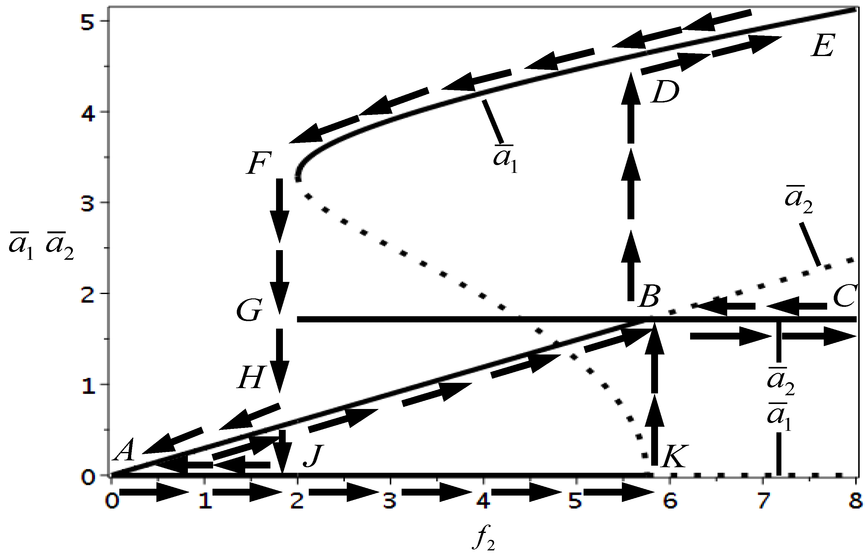
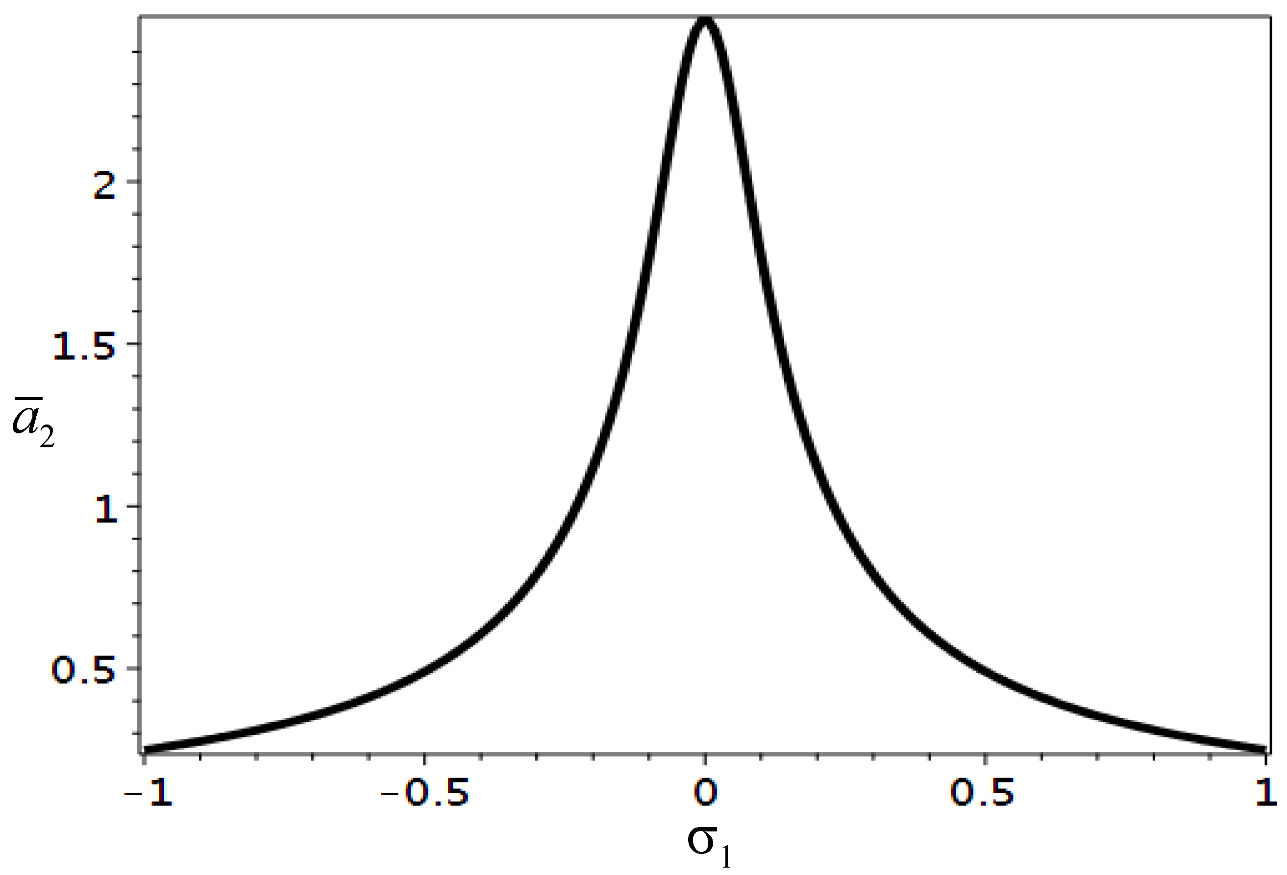
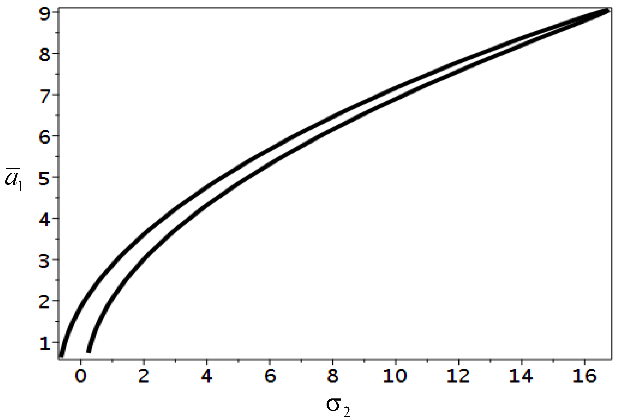
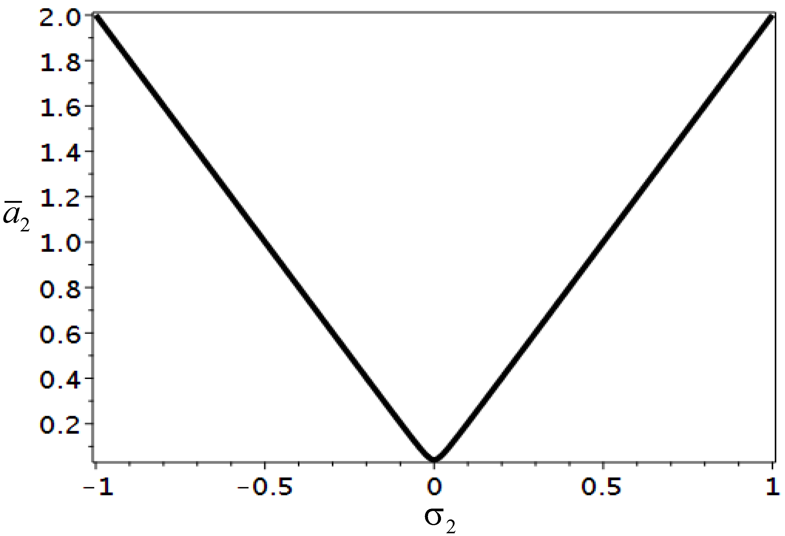
3. Three Equilibrium Configurations

Due to the residual thermal stress, the bistable composite laminated shell has three equilibrium configurations, which are two stable equilibrium configurations and one unstable equilibrium configuration. In order to determine the three equilibrium configurations, the time derivatives and dynamic load in Equations (27) and (28) are dropped. Making u₀ = v₀ = w₀ = 0, the static equations can be derived as follows:

$$\begin{array}{c}{A}_{11}\frac{{\partial }^2{u}_s}{\partial x^2}+\left(A_{12}+A_{66}\right)\frac{{\partial }^2{v}_s}{\partial x\partial y}+A_{16}\frac{{\partial }^2{v}_s}{\partial x^2}+2A_{16}\frac{{\partial }^2{u}_s}{\partial x\partial y}+A_{26}\frac{{\partial }^2{v}_s}{\partial y^2}+A_{66}\frac{{\partial }^2{u}_s}{\partial y^2}\hfill \\ -3B_{16}\frac{{\partial }^3{w}_s}{\partial x^2\partial y}-B_{26}\frac{{\partial }^3{w}_s}{\partial y^3}-\left(2B_{66}+B_{12}\right)\frac{{\partial }^3{w}_s}{\partial y^2\partial x}-B_{11}\frac{{\partial }^3{w}_s}{\partial x^3}+A_{26}\frac{\partial w_s}{\partial y}\frac{{\partial }^2{w}_s}{\partial y^2}\hfill \\ +\left(A_{66}+A_{12}\right)\frac{\partial w_s}{\partial y}\frac{{\partial }^2{w}_s}{\partial y\partial x}+A_{66}\frac{\partial w_s}{\partial x}\frac{{\partial }^2{w}_s}{\partial y^2}+A_{11}\frac{\partial w_s}{\partial x}\frac{{\partial }^2{w}_s}{\partial x^2}+A_{16}\frac{\partial w_s}{\partial y}\frac{{\partial }^2{w}_s}{\partial x^2}\hfill \\ +2A_{16}\frac{\partial w_s}{\partial x}\frac{{\partial }^2{w}_s}{\partial y\partial x}-\frac{\partial N_{xx}^T}{\partial x}-\frac{\partial N_{xy}^T}{\partial y}=0,\hfill \end{array}$$

(32)

$$\begin{array}{c}{A}_{66}\frac{{\partial }^2{v}_s}{\partial x^2}+\left(A_{12}+A_{66}\right)\frac{{\partial }^2{u}_s}{\partial x\partial y}+A_{16}\frac{{\partial }^2{u}_s}{\partial x^2}+2A_{16}\frac{{\partial }^2{v}_s}{\partial x\partial y}+A_{22}\frac{{\partial }^2{v}_s}{\partial y^2}+A_{26}\frac{{\partial }^2{u}_s}{\partial y^2}\hfill \\ -3B_{26}\frac{{\partial }^3{w}_s}{\partial y^2\partial x}-B_{16}\frac{{\partial }^3{w}_s}{\partial x^3}-\left(2B_{66}+B_{12}\right)\frac{{\partial }^3{w}_s}{\partial x^2\partial y}-B_{22}\frac{{\partial }^3{w}_s}{\partial y^3}+A_{22}\frac{\partial w_s}{\partial y}\frac{{\partial }^2{w}_s}{\partial y^2}\hfill \\ +\left(A_{66}+A_{12}\right)\frac{\partial w_s}{\partial x}\frac{{\partial }^2{w}_s}{\partial y\partial x}+A_{26}\frac{\partial w_s}{\partial x}\frac{{\partial }^2{w}_s}{\partial y^2}+A_{16}\frac{\partial w_s}{\partial x}\frac{{\partial }^2{w}_s}{\partial x^2}+A_{66}\frac{\partial w_s}{\partial y}\frac{{\partial }^2{w}_s}{\partial x^2}\hfill \\ +2A_{26}\frac{\partial w_s}{\partial x}\frac{{\partial }^2{w}_s}{\partial y\partial x}-\frac{\partial N_{yy}^T}{\partial y}-\frac{\partial N_{xy}^T}{\partial x}=0,\hfill \end{array}$$

(33)

$$\begin{array}{c}{B}_{11}(\frac{{\partial }^3{u}_s}{\partial x^3}+\frac{{\partial }^2{w}_s}{\partial x^2}\frac{{\partial }^2{w}_s}{\partial x^2}+\frac{\partial w_s}{\partial x}\frac{{\partial }^3{w}_s}{\partial x^3})+B_{12}(\frac{{\partial }^3{v}_s}{\partial x^2\partial y}+\frac{{\partial }^2{w}_s}{\partial x\partial y}\frac{{\partial }^2{w}_s}{\partial x\partial y}+\frac{\partial w_s}{\partial y}\frac{{\partial }^3{w}_s}{\partial x^2\partial y})\hfill \\ +B_{16}(\frac{{\partial }^3{u}_s}{\partial x^2\partial y}+\frac{{\partial }^3{v}_s}{\partial x^3}+\frac{\partial w_s}{\partial y}\frac{{\partial }^3{w}_s}{\partial x^3}+2\frac{{\partial }^2{w}_s}{x^2}\frac{{\partial }^2{w}_s}{\partial x\partial y}+\frac{\partial w_s}{\partial x}\frac{{\partial }^3{w}_s}{\partial x^2\partial y})-D_{11}\frac{{\partial }^4{w}_s}{\partial x^4}\hfill \\ -D_{12}\frac{{\partial }^4{w}_s}{\partial x^2\partial y^2}-D_{16}\frac{{\partial }^4{w}_s}{\partial x^3\partial y}+2B_{16}(\frac{{\partial }^3{u}_s}{\partial x^2\partial y}+\frac{{\partial }^2{w}_s}{\partial x^2}\frac{{\partial }^2{w}_s}{\partial x\partial y}+\frac{\partial w_s}{\partial x}\frac{{\partial }^3{w}_s}{\partial x^2\partial y})\hfill \\ +2B_{26}(\frac{{\partial }^3{v}_s}{\partial x\partial y^2}+\frac{{\partial }^2{w}_s}{\partial y^2}\frac{{\partial }^2{w}_s}{\partial x\partial y}+\frac{\partial w_s}{\partial y}\frac{{\partial }^3{w}_s}{\partial x\partial y^2})+B_{12}(\frac{{\partial }^3{u}_s}{\partial x\partial y^2}+\frac{{\partial }^2{w}_s}{\partial x\partial y}\frac{{\partial }^2{w}_s}{\partial x\partial y}+\frac{\partial w_s}{\partial x}\frac{{\partial }^3{w}_s}{\partial x\partial y^2})\hfill \\ +2B_{66}(\frac{{\partial }^3{u}_s}{\partial x\partial y^2}+\frac{{\partial }^2{w}_s}{\partial y^2}\frac{{\partial }^2{w}_s}{\partial x^2}+\frac{\partial w_s}{\partial y}\frac{{\partial }^3{w}_s}{\partial x^2\partial y}+\frac{{\partial }^3{v}_s}{\partial x^2\partial y}+\frac{{\partial }^2{w}_s}{\partial x\partial y}\frac{{\partial }^2{w}_s}{\partial x\partial y}+\frac{\partial w_s}{\partial x}\frac{{\partial }^3{w}_s}{\partial x\partial y^2})\hfill \\ -4D_{66}\frac{{\partial }^4{w}_s}{\partial x^2\partial y^2}+B_{22}(\frac{{\partial }^3{v}_s}{\partial y^3}+\frac{{\partial }^2{w}_s}{\partial y^2}\frac{{\partial }^2{w}_s}{\partial y^2}+\frac{\partial w_s}{\partial y}\frac{{\partial }^3{w}_s}{\partial y^3})-D_{12}\frac{{\partial }^4{w}_s}{\partial x^2\partial y^2}-D_{22}\frac{{\partial }^4{w}_s}{\partial y^4}\hfill \\ -D_{26}\frac{{\partial }^4{w}_s}{\partial x\partial y^3}+N\left(w_s\right)-(\frac{{\partial }^2{M}_{\mathrm{xx}}^T}{\partial x^2}+2\frac{{\partial }^2{M}_{\mathrm{xy}}^T}{\partial y\partial x}+\frac{{\partial }^2{M}_{\mathrm{yy}}^T}{\partial y^2})-2D_{16}\frac{{\partial }_4{w}_s}{\partial x^3\partial y}=0.\hfill \end{array}$$

(34)

Substituting Equations (21)–(23) into Equations (32)–(34) and taking two degrees of freedom, a set of static nonlinear equations are derived:

$$\begin{array}{c}{k}_1{w}_1+k_2{w}_2+N_1\left(\Delta T\right)w_1+N_2\left(\Delta T\right)w_2+{\mathsf{\alpha }}_1{w}_1^2+{\mathsf{\alpha }}_2{w}_2^2+{\mathsf{\alpha }}_3{w}_1{w}_2\\ +{\mathsf{\alpha }}_4{w}_1^3+{\mathsf{\alpha }}_5{w}_2^3+{\mathsf{\alpha }}_6{w}_1^2{w}_2+{\mathsf{\alpha }}_7{w}_1{w}_2^2+N_5\left(\Delta T\right)=0,\end{array}$$

(35)

$$\begin{array}{c}{k}_3{w}_1+k_4{w}_2+N_3\left(\Delta T\right)w_1+N_4\left(\Delta T\right)w_2+{\mathsf{\beta }}_1{w}_1^2+{\mathsf{\beta }}_2{w}_2^2+{\mathsf{\beta }}_3{w}_1{w}_2\\ +{\mathsf{\beta }}_4{w}_1^3+{\mathsf{\beta }}_5{w}_2^3+{\mathsf{\beta }}_6{w}_1^2{w}_2+{\mathsf{\beta }}_7{w}_1{w}_2^2+N_6\left(\Delta T\right)=0.\end{array}$$

(36)

Changing the variable parameter ΔΤ, a series of static solutions for the equilibrium configurations can be derived, which form static bifurcation diagrams shown in Figure 2. In Figure 2, (a) donates the static bifurcation curve of w₁ which represents x-curvature, (b) donates the static bifurcation curve of w₂ which represents y-curvature.

The asymmetric composite laminated plate starts almost flatly at the elevated manufacturing temperature, point A in Figure 2. As the elevated manufacturing temperature increases, small curvatures develop. The curvatures are equal in magnitude but opposite in symbol, which indicates that the composite laminated plate warps, forming a shallow saddle shell. At point B, the curve of curvature-temperature relationship bifurcates into three paths BC, BD and BE, which represent curvatures in three cases. Along the path BC, the y-curvature increases while the x-curvature decreases. That is to say, the y-curvature dominates along the path BC, leading to one stable cylindrical equilibrium configuration. Along the path BE, the x-curvature increases while the y-curvature decreases. That is to say, the x-curvature dominates along the path BE, leading to another one stable cylindrical equilibrium configuration. Along the path BD, the x and y-curvatures increase slightly and remain equal in magnitude but opposite in symbol. Point D corresponds to the unstable saddle equilibrium configuration. It is concluded from Figure 2 that the number of equilibrium solutions varies from 1 to 3 with the change of parameter ΔΤ. The static bifurcation called supercritical pitchfork bifurcation occurs in the formation process of the bi-stability.

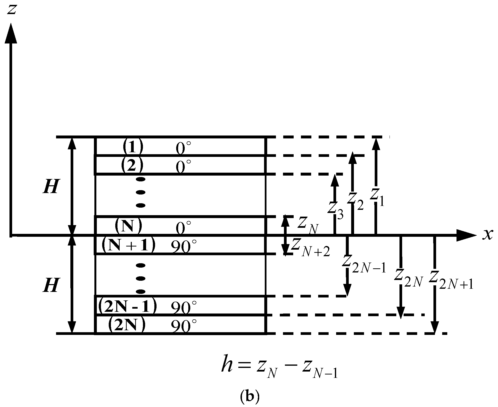
4. Equation of Motion for Local Dynamics

When subjected to the base excitation with small amplitudes, the bistable shell vibrates around just one stable configuration, which are defined as local dynamics. All vibrations confined to a single stable configuration behave as 1:2 internal resonance, saturation and penetration.

For local dynamics around one of the two stable equilibrium configurations, the above relationships will have to be redefined.

The nonlinear strain–displacement relations are rewritten as follows:

$$\left\{\begin{array}{c}{\mathsf{\epsilon }}_{xx}\\ {\mathsf{\epsilon }}_{yy}\\ {\mathsf{\epsilon }}_{xy}\end{array}\right\}=\left\{\begin{array}{c}{\mathsf{\epsilon }}_{xx}^{\left(0\right)}\\ {\mathsf{\epsilon }}_{yy}^{\left(0\right)}\\ {\gamma }_{xy}^{\left(0\right)}\end{array}\right\}+z\left\{\begin{array}{c}{\mathsf{\epsilon }}_{xx}^{\left(1\right)}\\ {\mathsf{\epsilon }}_{yy}^{\left(1\right)}\\ {\gamma }_{xy}^{\left(1\right)}\end{array}\right\}$$

(37)

$$\left\{\begin{array}{c}{\mathsf{\epsilon }}_{xx}^{\left(0\right)}\\ {\mathsf{\epsilon }}_{yy}^{\left(0\right)}\\ {\gamma }_{xy}^{\left(0\right)}\end{array}\right\}=\left\{\begin{array}{c}\frac{\partial u_0}{\partial x}+\frac{1}{2}{\left(\frac{\partial w_0}{\partial x}\right)}^2+\frac{w_0}{R_1}\\ \frac{\partial v_0}{\partial y}+\frac{1}{2}{\left(\frac{\partial w_0}{\partial y}\right)}^2+\frac{w_0}{R_2}\\ \frac{\partial u_0}{\partial y}+\frac{\partial v_0}{\partial x}+\frac{\partial w_0}{\partial x}\frac{\partial w_0}{\partial y}\end{array}\right\}, \left\{\begin{array}{c}{\mathsf{\epsilon }}_{xx}^{\left(1\right)}\\ {\mathsf{\epsilon }}_{yy}^{\left(1\right)}\\ {\gamma }_{xy}^{\left(1\right)}\end{array}\right\}=\left\{\begin{array}{c}-\frac{{\partial }^2{w}_0}{\partial x^2}\\ -\frac{{\partial }^2{w}_0}{\partial y^2}\\ -2\frac{{\partial }^2{w}_0}{\partial x\partial y}\end{array}\right\},$$

(38)

where R₁ and R₂ are radii of curvatures of one of the two stable equilibrium configurations corresponding to the initial curvatures $\frac{{\partial }^2{w}_s}{\partial x^2}$ and $\frac{{\partial }^2{w}_s}{\partial y^2}$ determined above.

Using Equations (7), (8), (37) and (38), the strain energy can be rewritten as follows:

$$U=\frac{1}{2}{\displaystyle {\int }_{-L_x}^{L_x}{\displaystyle {\int }_{-L_y}^{L_y}\left[\begin{array}{cc}{\mathsf{\epsilon }}^{\left(0\right)}& {\mathsf{\epsilon }}^{\left(1\right)}\end{array}\right]}}\left[\begin{array}{cc}\left[A\right]& \left[B\right]\\ \left[B\right]& \left[D\right]\end{array}\right]\left[\begin{array}{c}{\mathsf{\epsilon }}^{\left(0\right)}\\ {\mathsf{\epsilon }}^{\left(1\right)}\end{array}\right]dxdy.$$

(39)

The kinetic energy can be rewritten as follows:

$$K=\frac{1}{2}\mathsf{\sum }\mathsf{\rho }\underset{\Omega }{\int }{\int }_{{-}_H}^H\left({\stackrel{.}{u}}^2+{\stackrel{.}{v}}^2+{\stackrel{.}{w}}^2\right)dxdydz.$$

(40)

By using Chebyshev polynomials, u₀, v₀ and w₀ are expanded as follows:

$$u_0(x,y,t)=R^u(x,y)U(x,y)r\left(t\right),$$

(41)

$$v_0(x,y,t)=R^v(x,y)V(x,y)r\left(t\right),$$

(42)

$$w_0(x,y,t)=R^w(x,y)W(x,y)r\left(t\right),$$

(43)

where R^u(x,y), R^v(x,y) and R^w(x,y) are boundary functions, U(x,y), V(x,y) and W(x,y) are spatial functions and r(t) is a temporal function.

The boundary functions can be expressed as follows:

$$R^{\mathsf{\alpha }}\left(x,y\right)={\left(1+\frac{2x}{L_x}\right)}^p{\left(1-\frac{2x}{L_x}\right)}^q{\left(1+\frac{2y}{L_y}\right)}^r{\left(1-\frac{2y}{L_y}\right)}^s,$$

(44)

where α = u, v, w. p, q, r, s depends on the constraint boundaries of the bistable shell and are equal to either 0 or 1. Different values of the boundary functions are shown in

Table 2. Different values of the boundary functions.

	Ru(x)	Rv(x)	Rw(x)	Ru(y)	Rv(y)	Rw(y)
FFFF	1	1	1	1	1	1
FSFF	1	1 − x	1 − x	1 − y	1	1 − y
SFFF	1	1 + x	1 + x	1 + y	1	1 + y
SSFF	1	1 − x2	1 − x2	1 − y2	1	1 − y2
FCFF	1 − x	1 − x	1 − x	1 − y	1 − y	1 − y
CFFF	1 + x	1 + x	1 + x	1 + y	1 + y	1 + y
SCFF	1 − x	1 − x2	1 − x2	1 − y2	1 − y	1 − y2
CSFF	1 + x	1 − x2	1 − x2	1 − y2	1 + y	1 − y2
CCFF	1 − x2	1 − x2	1 − x2	1 − y2	1 − y2	1 − y2

.

As the four edges of the shell are free, R^α(x,y) = 0. The shape functions are expressed as:

$$U(\xi ,\mathsf{\eta })=\sum _{m=0}^M\sum _{n=0}^N{U}_{m,n}{T}_m(2\xi -1)T_n(2\mathsf{\eta }-1),$$

(45)

$$V(\xi ,\mathsf{\eta })=\sum _{m=0}^M\sum _{n=0}^N{V}_{m,n}{T}_m(2\xi -1)T_n(2\mathsf{\eta }-1),$$

(46)

$$W(\xi ,\mathsf{\eta })=\sum _{m=0}^M\sum _{n=0}^N{W}_{m,n}{T}_m(2\xi -1)T_n(2\mathsf{\eta }-1),$$

(47)

where T_m and T_n are the m-th and n-th order Chebyshev polynomial of the first kind, respectively.

As the vibration exciter itself is composed of a series of spring components, when the shell is subjected to the base excitation with small amplitudes by the vibration exciter, the local dynamics confined to one stable configuration occur and the vibration behavior of the system is similar to that of a spring-mass system. That is to say, the local dynamics around one stable configuration need to take additional spring stiffness due to the vibration exciter into account [38,40]. Therefore, the additional stiffness is applied to the supporting bar, through which the shell and vibration exciter are connected. In this case, it is assumed that the center of the shell is elastically supported and the four edges are free.

The additional elastic potential energy due to the vibration exciter is given by:

$$U_b=\frac{1}{2}{k}_b{w}_0^2\left(0,0\right),$$

(48)

where k_b is the additional stiffness caused by the supporting bar.

The total strain energy is thus:

$$U_{\mathrm{total}}=U+U_b.$$

(49)

The Rayleigh–Ritz method is used, and the following equation is applied:

$$\frac{\partial \left(K-U_{\mathrm{total}}\right)}{\partial \mathrm{p}}=0,$$

(50)

where:

$$\mathrm{p}=\left\{U_{11} , \dots , U_{MN} , V_{11} , \dots , V_{MN} , W_{11} , \dots , W_{MN} \right\}.$$

(51)

Substituting Equations (37)–(49) into Equation (50), Equation (50) is expressed in the form of matrix:

$$(\mathbf{K}-{\mathsf{\omega }}^2\mathbf{M})\mathrm{p}=0,$$

(52)

where K and M represent stiffness matrix and mass matrix respectively, p is n-dimensional displacement vector and n = 3MN.

The eigenvalues of matrix (52) are solved to derive the natural frequencies and the eigenvalues are brought back to matrix (52) to obtain the corresponding eigenvectors, so as to calculate the shape functions:

$$U^{\left(i\right)}\left(\xi ,\mathsf{\eta }\right)={\displaystyle \sum _{m=0}^M{\displaystyle \sum _{n=0}^N{U}_{m,n}^{\left(i\right)}{T}_m}}\left(2\xi -1\right)T_n\left(2\mathsf{\eta }-1\right),$$

(53)

$$V^{\left(i\right)}\left(\xi ,\mathsf{\eta }\right)={\displaystyle \sum _{m=0}^M{\displaystyle \sum _{n=0}^N{V}_{m,n}^{\left(i\right)}{T}_m}}\left(2\xi -1\right)T_n\left(2\mathsf{\eta }-1\right),$$

(54)

$$W^{\left(i\right)}\left(\xi ,\mathsf{\eta }\right)={\displaystyle \sum _{m=0}^M{\displaystyle \sum _{n=0}^N{W}_{m,n}^{\left(i\right)}{T}_m}}\left(2\xi -1\right)T_n\left(2\mathsf{\eta }-1\right),$$

(55)

Then the corresponding modal functions can be determined:

$$u_0\left(\xi ,\mathsf{\eta },t\right)={\displaystyle \sum _{j=J}^{\tilde{M}}{u}_j\left(t\right)}{U}^{\left(j\right)}\left(\xi ,\mathsf{\eta }\right), i=1,\dots ,\overline{\mathbf{M}}, j=\mathrm{J},\dots ,\tilde{\mathbf{M}},$$

(56)

$$v_0\left(\xi ,\mathsf{\eta },t\right)={\displaystyle \sum _{j=J}^{\tilde{M}}{v}_j\left(t\right)}{V}^{\left(j\right)}\left(\xi ,\mathsf{\eta }\right), i=1,\dots ,\overline{\mathbf{M}}, j=\mathrm{J},\dots ,\tilde{\mathbf{M}},$$

(57)

$$w_0\left(\xi ,\mathsf{\eta },t\right)={\displaystyle \sum _{i=1}^{\overline{M}}{w}_j\left(t\right)}{W}^{\left(i\right)}\left(\xi ,\mathsf{\eta }\right), i=1,\dots ,\overline{\mathbf{M}}, j=\mathrm{J},\dots ,\tilde{\mathbf{M}}.$$

(58)

According to Hamilton’s principle, the equations for the local dynamics can be obtained:

$$\frac{\partial N_{xx}}{\partial x}+\frac{\partial N_{xy}}{\partial y}=I_0\frac{{\partial }^2{u}_0}{\partial t^2}-I_1\frac{{\partial }^2}{\partial t^2}\left(\frac{\partial w_0}{\partial x}\right),$$

(59)

$$\frac{\partial N_{xy}}{\partial x}+\frac{\partial N_{yy}}{\partial y}=I_0\frac{{\partial }^2{v}_0}{\partial t^2}-I_1\frac{{\partial }^2}{\partial t^2}\left(\frac{\partial w_0}{\partial y}\right),$$

(60)

$$\begin{array}{c}\frac{{\partial }^2{M}_{xx}}{\partial x^2}+2\frac{{\partial }^2{M}_{xy}}{\partial y\partial x}+\frac{{\partial }^2{M}_{yy}}{\partial y^2}-\frac{N_{xx}}{R_x}-\frac{N_{yy}}{R_y}+N\left(w_0\right)=I_0\frac{{\partial }^2{w}_0}{\partial t^2}+I_0\frac{{\partial }^{2}Y}{\partial t^2}\\ -I_2\frac{{\partial }^2}{\partial t^2}(\frac{{\partial }^2{w}_0}{\partial x^2}+\frac{{\partial }^2{w}_0}{\partial y^2})+I_1\frac{{\partial }^2}{\partial t^2}(\frac{\partial u_0}{\partial x}+\frac{\partial v_0}{\partial y}),\end{array}$$

(61)

where:

$$N\left(w_0\right)=\frac{\partial }{\partial x}\left(N_{xx}\frac{\partial w_0}{\partial x}+N_{xy}\frac{\partial w_0}{\partial y}\right)+\frac{\partial }{\partial y}\left(N_{xy}\frac{\partial w_0}{\partial x}+N_{yy}\frac{\partial w_0}{\partial y}\right).$$

(62)

In order to analyze local dynamics with the extra stiffness caused by the exciter around one of the two stable equilibrium configurations, the initial curvatures $\frac{{\partial }^2{w}_s}{\partial x^2}$ and $\frac{{\partial }^2{w}_s}{\partial y^2}$ of the second stable equilibrium configuration according to the previous section are transformed into the radii of curvatures R₁ and R₂ of the cylindrical shell. The Rayleigh–Ritz method is used to determine the modal shapes for the boundary conditions of central elastic support, as shown in Figure 3.

In order to analyze local dynamics with the extra stiffness caused by the exciter around one of the two stable equilibrium configurations, the initial curvatures $\frac{{\partial }^2{w}_s}{\partial x^2}$ and $\frac{{\partial }^2{w}_s}{\partial y^2}$ of the second stable equilibrium configuration according to the previous section are transformed into the radii of curvatures R₁ and R₂ of the cylindrical shell. The Rayleigh–Ritz method is used to determine the modal shapes for the boundary conditions of central elastic support, as shown in Figure 3.

Substituting Equations (56)–(58) into Equations (59)–(61), selecting the first two modal functions and using the Galerkin approach, two degree of freedom ordinary differential equations are determined as:

$${\ddot{w}}_1+c{\dot{w}}_1+{\mathsf{\omega }}_1^2{w}_1+{\mathsf{\alpha }}_{11}{w}_1^2+{\mathsf{\alpha }}_{12}{w}_2^2+{\mathsf{\alpha }}_{13}{w}_1{w}_2={\gamma }_1\ddot{Y},$$

(63)

$${\ddot{w}}_2+c{\dot{w}}_2+{\mathsf{\omega }}_2^2{w}_2+{\mathsf{\beta }}_{11}{w}_1^2+{\mathsf{\beta }}_{12}{w}_2^2+{\mathsf{\beta }}_{13}{w}_1{w}_2={\gamma }_2\ddot{Y}.$$

(64)

Dimensionless variables are introduced:

$${\overline{w}}_1=\frac{w_1}{L_x}, {\overline{w}}_2=\frac{w_2}{L_y}, \overline{x}=\frac{x}{L_x}, \overline{y}=\frac{y}{L_y}, \overline{t}={\mathsf{\omega }}_{1}t, \overline{\mathsf{\Omega }}=\frac{\mathsf{\Omega }}{{\mathsf{\omega }}_1}.$$

(65)

By using Equation (65), dimensionless equations can be derived:

$${\ddot{\overline{w}}}_1+{\overline{c}}_1{\dot{\overline{w}}}_1+{\overline{\mathsf{\omega }}}_1^2{\overline{w}}_1+{\overline{\mathsf{\alpha }}}_1{\overline{w}}_1^2+{\overline{\mathsf{\alpha }}}_2{\overline{w}}_2^2+{\overline{\mathsf{\alpha }}}_3{\overline{w}}_1{\overline{w}}_2={\overline{\gamma }}_1\overline{f}\cos \left(\overline{\mathsf{\Omega }}\overline{t}\right),$$

(66)

$${\ddot{\overline{w}}}_2+{\overline{c}}_2{\dot{\overline{w}}}_2+{\overline{\mathsf{\omega }}}_2^2{\overline{w}}_2+{\overline{\mathsf{\beta }}}_1{\overline{w}}_1^2+{\overline{\mathsf{\beta }}}_2{\overline{w}}_2^2+{\overline{\mathsf{\beta }}}_3{\overline{w}}_1{\overline{w}}_2={\overline{\gamma }}_2\overline{f}\cos \left(\overline{\mathsf{\Omega }}\overline{t}\right).$$

(67)

5. Numerical Simulation

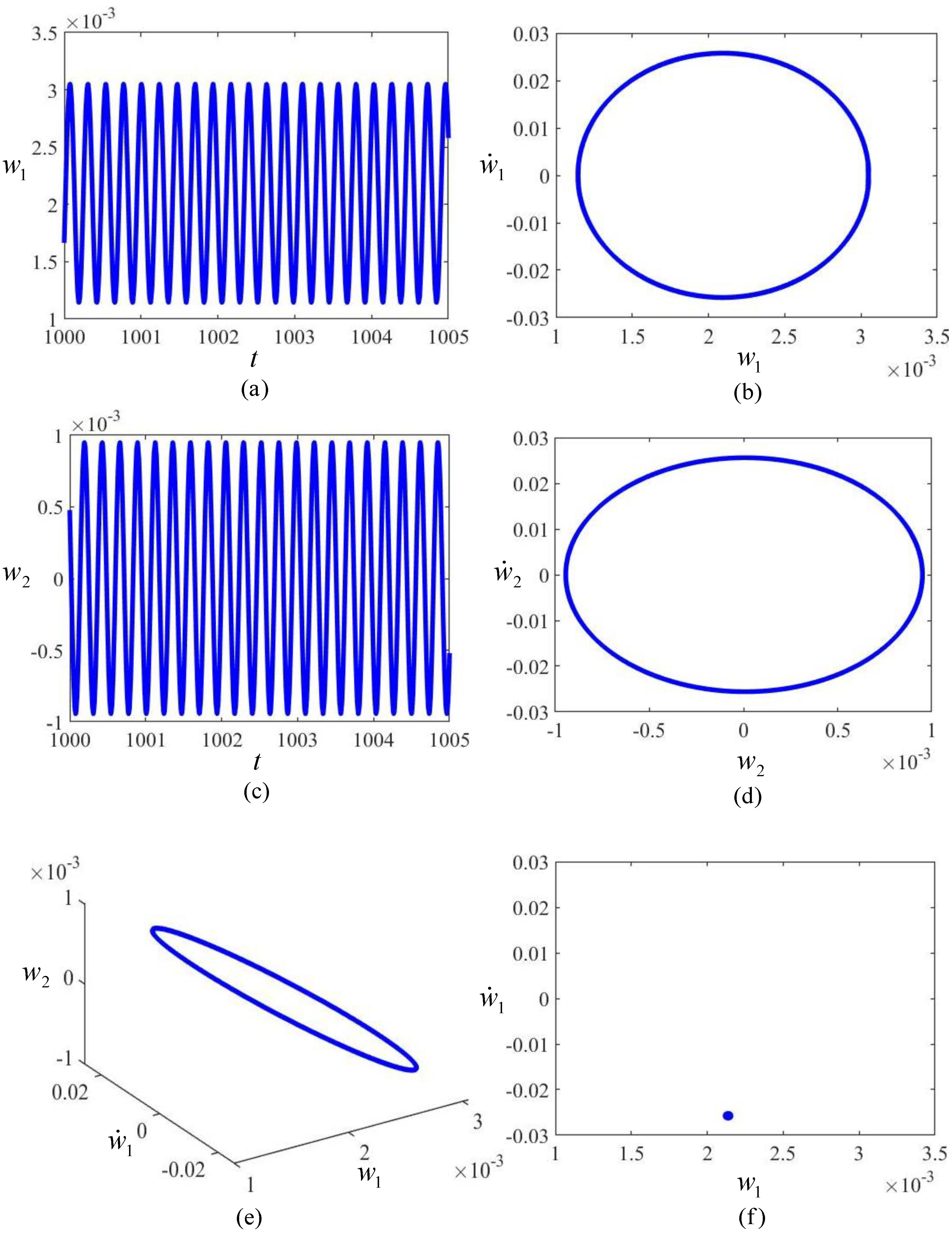
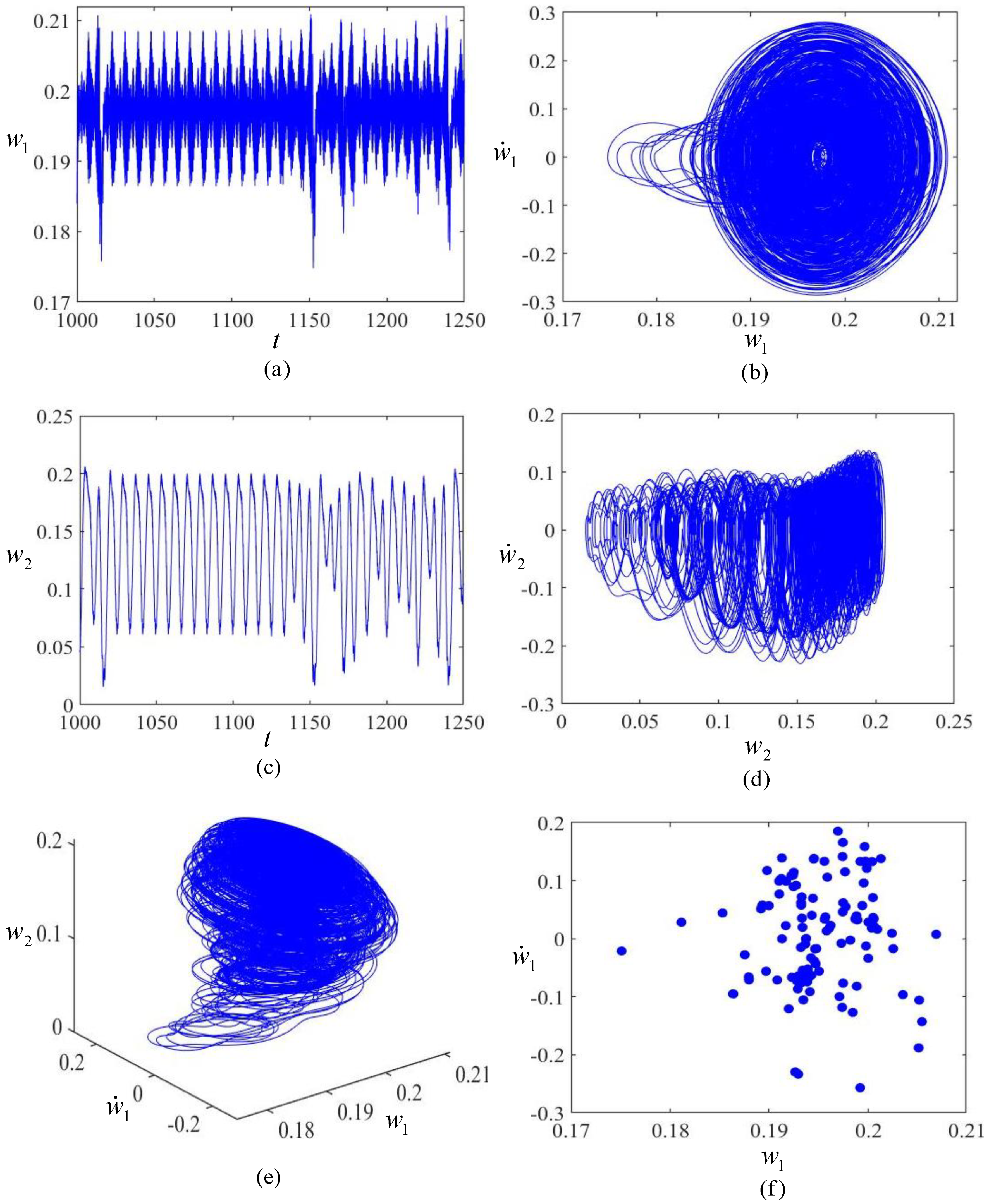
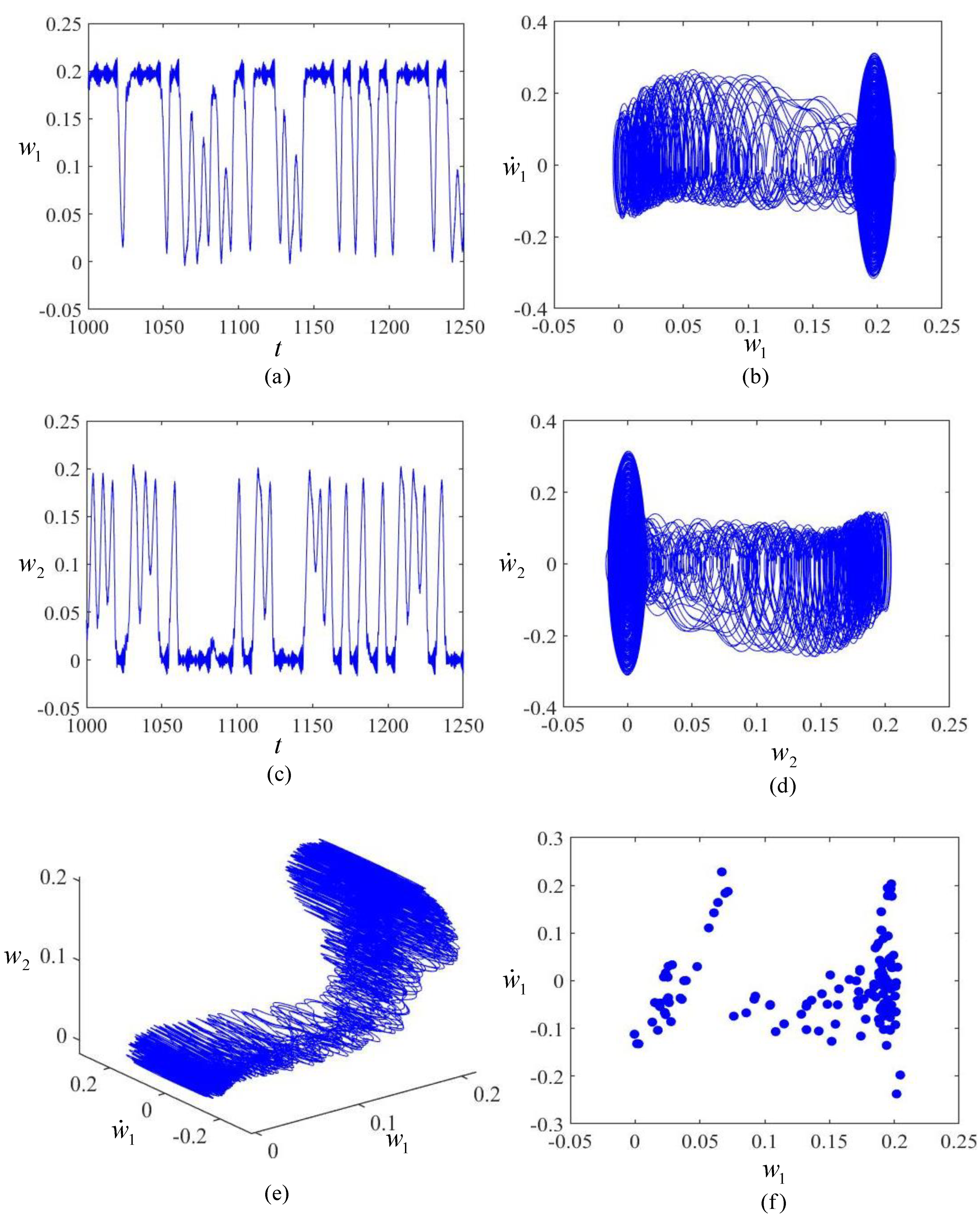
5.1. Global Dynamics

To study the global dynamics, the fifth-order Runge–Kutta algorithm is adopted to solve Equations (30) and (31), which demonstrates the bifurcation diagram, the phase portrait, the time-history graph and the Poincaré map. For convenience in this study, the overbars in Equations (30) and (31) are dropped in the following analysis.

(a) donates the time-history on the plane $\left(t,w_1\right)$, (b) donates the phase portrait on the plane $\left(w_1,{\dot{w}}_1\right)$, (c) donates the time-history on the plane $\left(t,w_2\right)$, (d) donates the phase portrait on the plane $\left(w_2,{\dot{w}}_2\right)$, (e) donates three-dimensional phase portrait in space $\left(w_1,{\dot{w}}_1,w_2\right)$ and (f) donates Poincaré map on the plane $\left(w_1,{\dot{w}}_1\right)$, which are shown in Figure 4, Figure 5, Figure 6, Figure 7, Figure 8, Figure 9 and Figure 10 respectively. The vibration form is judged by distribution of points in Poincaré map. When the Poincaré map shows only one point, periodic vibration is determined. When the Poincaré map shows a closed curve, quasi-periodic vibration is determined. When the Poincaré map shows a large cluster of points, chaotic vibration is determined.

w₁ represents the vibration for curvature in the x direction while w₂ represents the vibration for curvature in the y direction. Through the comparative study of w₁ and w₂, the vibrations of the bistable shell can be determined. When f = 0.2, w₁ and w₂ remain almost zero around the equilibrium position (0, 0), that is to say, the bistable shell vibrates slightly around the first stable equilibrium configuration, which is the periodic vibration according to Poincaré map shown in Figure 4. When f = 0.35, w₁ increases rapidly while w₂ remain almost zero around the equilibrium position (0, 0),that is to say, the bistable shell vibrates violently around the first stable equilibrium configuration, which is the chaotic vibration according to Poincaré map shown in Figure 5. When f = 0.425, in a phase after the start, w₁ increases rapidly while w₂ remain almost zero around the equilibrium position (0, 0), at a certain moment, w₁ increases from 0 to 0.2 and remains almost constant while w₂ increases from 0 to 0.2 and vibrates violently around the equilibrium position (0.2, 0.2), that is to say, dynamic snap-through occurs, which is the chaotic vibration according to the Poincaré map shown in Figure 6. When f = 0.43, w₁ and w₂ vibrate violently around the equilibrium position (0.2, 0.2), that is to say, the bistable shell vibrates violently around the second stable equilibrium configuration, which is the chaotic vibration according to the Poincaré map shown in Figure 7. When f = 0.5, w₁ and w₂ change repeatedly between 0 and 0.2 simultaneously, namely, the constant dynamic snap-through occurs between the two stable equilibrium configurations, which is the chaotic vibration according to the Poincaré map shown in Figure 8. When f = 0.8, w₁ vibrates slightly while w₂ remain almost zero around the equilibrium position (0, 0), that is to say, the bistable shell vibrates slightly around the first stable equilibrium configuration, which is the quasi-periodic vibration according to the Poincaré map shown in Figure 9. When f = 0.9, w₁ and w₂ remain almost 0.2 around the equilibrium position (0.2, 0.2), that is to say, the bistable shell vibrates slightly around the second stable equilibrium configuration, which is the periodic vibration according to the Poincaré map shown in Figure 10.

In order to understand the influence of excitation amplitude f on global dynamics more comprehensively, make f locate in a range of 0~1.2 and bifurcation diagrams can be obtained shown in Figure 11.

In Figure 11, when f is located in the interval 0~0.25, w₁ and w₂ vibrate slightly around the equilibrium position (0, 0), when f is located in the interval 0.25~0.43, w₁ and w₂ vibrate violently around the equilibrium position (0, 0), when f is located in the interval 0.43~0.72, w₁ and w₂ vibrate violently between the equilibrium positions (0, 0)and (0.2, 0.2) and when f is located in the interval 0.72~1.2, w₁ and w₂ vibrate slightly around the equilibrium position (0, 0) or (0.2, 0.2).

Combined with the vibration and Poincaré map shown in Figure 4, Figure 5, Figure 6, Figure 7, Figure 8, Figure 9 and Figure 10 respectively, we can find from Figure 11 that the vibration of the bistable shell changes from the periodic vibration around the first stable equilibrium configuration → the quasi-periodic vibration around the first stable equilibrium configuration → the chaotic vibration around the first stable equilibrium configuration → the snap-through and chaotic vibration between the two stable equilibrium configurations→ the constant snap-through and chaotic vibration between the two stable equilibrium configurations → the quasi-periodic vibration around the second stable equilibrium configuration → the periodic vibration around the second stable equilibrium configuration when the excitation amplitude f changes from 0 to 1.2. From another point of view, it is seen from Figure 11 that the vibration of the bistable asymmetric composite laminated shell changes from the vibration with small amplitude around the first stable equilibrium configuration → the oscillation with large amplitude around the first stable equilibrium configuration → the oscillation with large amplitude between the two stable equilibrium configurations → the oscillation with large amplitude around the second stable equilibrium configuration → the vibration with small amplitude around the second stable equilibrium configuration.

Figure 8 and Figure 11 exhibit the global dynamics. The global dynamics consist of the vibrations around the two stable equilibrium configurations respectively, which can be taken as the local dynamics and dynamic snap-through between the two stable equilibrium configurations. In other words, Figure 8 and Figure 11 exhibit dynamic snap-through and nonlinear vibrations with two potential wells.

5.2. Local Dynamics

For convenience, the overbars are dropped in Equations (63) and (64). Considering the case of primary parametric and 1:2 internal resonance, the resonant relations are given by:

$${\mathsf{\omega }}_2=2{\mathsf{\omega }}_1-\mathsf{\epsilon }{\mathsf{\sigma }}_2, \mathsf{\Omega }={\mathsf{\omega }}_2+\mathsf{\epsilon }{\mathsf{\sigma }}_1,$$

(68)

where σ₁ and σ₂ are two detuning parameters.

Small parameter variable ε is introduced:

$$\begin{array}{c}{c}_1\to \mathsf{\epsilon }{c}_1, c_2\to \mathsf{\epsilon }{c}_2, {\mathsf{\alpha }}_1\to \mathsf{\epsilon }{\mathsf{\alpha }}_1, {\mathsf{\alpha }}_2\to \mathsf{\epsilon }{\mathsf{\alpha }}_2, {\mathsf{\alpha }}_3\to \mathsf{\epsilon }{\mathsf{\alpha }}_3, {\mathsf{\beta }}_1\to \mathsf{\epsilon }{\mathsf{\beta }}_1, {\mathsf{\beta }}_2\to \mathsf{\epsilon }{\mathsf{\beta }}_2,\\ {\mathsf{\beta }}_3\to \mathsf{\epsilon }{\mathsf{\beta }}_3, {\gamma }_1\to \mathsf{\epsilon }{\gamma }_1, {\gamma }_2\to \mathsf{\epsilon }{\gamma }_2.\end{array}$$

(69)

Using Equations (68) and (69) and the method of multiple scales, Equations (63) and (64) are averaged as follows:

$$D_1{a}_1+c_1{a}_1+\frac{{\mathsf{\alpha }}_{14}}{4{\mathsf{\omega }}_1}{a}_1{a}_2\sin {\mathsf{\varphi }}_2=0,$$

(70)

$$D_1{a}_2+c_2{a}_2-\frac{{\mathsf{\beta }}_{11}}{4{\mathsf{\omega }}_2}{a}_1^2\sin {\mathsf{\varphi }}_2-\frac{{\gamma }_2{f}_2}{2{\mathsf{\omega }}_2}\sin {\mathsf{\varphi }}_1=0,$$

(71)

$$a_1{D}_1{\mathsf{\varphi }}_1-{\mathsf{\sigma }}_1{a}_2+\frac{{\mathsf{\beta }}_{11}}{4{\mathsf{\omega }}_2}{a}_1^2\cos {\mathsf{\varphi }}_2-\frac{{\gamma }_2{f}_2}{2{\mathsf{\omega }}_2}\cos {\mathsf{\varphi }}_1=0,$$

(72)

$$a_2{D}_1{\mathsf{\varphi }}_2+{\mathsf{\sigma }}_2{a}_2+(\frac{{\mathsf{\alpha }}_{14}}{2{\mathsf{\omega }}_1}{a}_2^2-\frac{{\mathsf{\beta }}_{11}}{4{\mathsf{\omega }}_2}{a}_1^2)\cos {\mathsf{\varphi }}_2-\frac{{\gamma }_2{f}_2}{2{\mathsf{\omega }}_2}\cos {\mathsf{\varphi }}_1=0,$$

(73)

where a₁ and a₂ represent the amplitude of w₁ and w₂ respectively and φ₁ and φ₂ and ${\mathsf{\varphi }}_2$ represent the phase angle of w₁ and w₂ respectively.

Let the derivatives at the left end of Equations (70)–(73) be zero as follows:

$$c_1{\overline{a}}_1+\frac{{\mathsf{\alpha }}_{14}}{4{\mathsf{\omega }}_1}{\overline{a}}_1{\overline{a}}_2\sin {\mathsf{\varphi }}_2=0,$$

(74)

$$c_2{\overline{a}}_2-\frac{{\mathsf{\beta }}_{11}}{4{\mathsf{\omega }}_2}{\overline{a}}_1^2\sin {\mathsf{\varphi }}_2-\frac{{\gamma }_2{f}_2}{2{\mathsf{\omega }}_2}\sin {\mathsf{\varphi }}_1=0,$$

(75)

$${\mathsf{\sigma }}_1{\overline{a}}_2-\frac{{\mathsf{\beta }}_{11}}{4{\mathsf{\omega }}_2}{\overline{a}}_1^2\cos {\mathsf{\varphi }}_2+\frac{{\gamma }_2{f}_2}{2{\mathsf{\omega }}_2}\cos {\mathsf{\varphi }}_1=0,$$

(76)

$${\mathsf{\sigma }}_2{\overline{a}}_2+(\frac{{\mathsf{\alpha }}_{14}}{2{\mathsf{\omega }}_1}{\overline{a}}_2^2-\frac{{\mathsf{\beta }}_{11}}{4{\mathsf{\omega }}_2}{\overline{a}}_1^2)\cos {\mathsf{\varphi }}_2-\frac{{\gamma }_2{f}_2}{2{\mathsf{\omega }}_2}\cos {\mathsf{\varphi }}_1=0,$$

(77)

The solutions of Equations (74)–(77) are divided into two sets by whether ${\overline{a}}_1$ is zero or not.

When ${\overline{a}}_1=0$, the first set of solutions is:

$${\overline{a}}_1=0, {\overline{a}}_2=\frac{{\gamma }_2{f}_2}{2{\mathsf{\omega }}_2\sqrt{c_2^2+{\mathsf{\sigma }}_1^2}}.$$

(78)

When ${\overline{a}}_1\ne 0$, the second set of solutions satisfies the following relation:

$$\begin{array}{c}{\mathsf{\omega }}_1^2{\mathsf{\beta }}_1^2\left[c_1^2+{\left(\frac{{\mathsf{\sigma }}_2-{\mathsf{\sigma }}_1}{2}\right)}^2\right]{\overline{a}}^4-{\mathsf{\omega }}_1{\mathsf{\omega }}_2{\mathsf{\alpha }}_{14}{\mathsf{\beta }}_1\left[2c_1{c}_2+{\mathsf{\sigma }}_1\left({\mathsf{\sigma }}_2-{\mathsf{\sigma }}_1\right)\right]{\overline{a}}_1^2{\overline{a}}_2^2\\ +{\mathsf{\omega }}_2^2{\mathsf{\alpha }}_{14}^2\left(c_2^2+{\mathsf{\sigma }}_1^2\right){\overline{a}}_2^4={\left(\frac{{\mathsf{\alpha }}_{14}{\overline{a}}_2{\gamma }_2{f}_2}{2}\right)}^2.\end{array}$$

(79)

Solving Equation (79) and considering Equation (78), a series of solutions can be determined shown in Figure 12, Figure 13, Figure 14, Figure 15, Figure 16 and Figure 17.

Figure 12 shows the force-amplitude curve for σ₂ = 0. In Figure 12, solid lines AK, FE and dotted line KF represent the amplitude ${\overline{a}}_1$ of the first mode and solid lines AB, GC and dotted line KF represent the amplitude ${\overline{a}}_2$ of the second mode. When the base excitation amplitude f₂ increases gradually from zero, ${\overline{a}}_1$ changes along AK and ${\overline{a}}_2$ changes along AB. When f₂ = 5.8, ${\overline{a}}_1$ transfers from AK to DE by snap-through and ${\overline{a}}_2$ transfers from AB to BC. When the base excitation amplitude f₂ decreases gradually from 8, ${\overline{a}}_1$ changes along EF and ${\overline{a}}_2$ changes along CG. When f₂ = 2, ${\overline{a}}_1$ transfers from EF to JA by snap-through and ${\overline{a}}_2$ transfers from CG to HA by snap-through. When ${\overline{a}}_2$ goes along CG, no matter how f₂ changes, ${\overline{a}}_2$ remains constant, that is to say, the response of the second mode enters saturation state. This is because the energy applied to the second mode is transferred to the first mode, which means that permeation takes place. Saturation and permeation are the peculiar phenomena of forced vibration of nonlinear multi-degree of freedom system related to 1:2 internal resonance.

Figure 13 shows the force-amplitude curve for σ₁ = σ₂ = 0. Similar to Figure 12, with the change of base excitation amplitude f₂, saturation and permeation occur.

Figure 14 is the frequency-amplitude curve of the first mode with respect to σ₁. It can be seen from Figure 14 that when σ₁ changes from negative to positive, the system shows the softening and hardening nonlinearity successively.

Figure 15 is the frequency-amplitude curve of the second mode with respect to σ₁. Different from Figure 14, with the change of σ₁, the system shows only linear characteristics.

Figure 16 is the frequency-amplitude curve of the first mode with respect to σ₂. It can be seen from Figure 16 that with the change of σ₂, the system shows the hardening nonlinearity.

Figure 17 is the frequency-amplitude curve of the second mode with respect to σ₂. It can be seen from Figure 17 that when σ₂ changes from negative to zero, the system shows the linear characteristics with negative slope, while when σ₂ changes from zero to positive, the system shows the linear characteristics with positive slope.

It can be found from Figure 12, Figure 13, Figure 14, Figure 15, Figure 16 and Figure 17 that when only the base excitation amplitude is changed, the system may have saturation and penetration, and when only the detuning parameter σ₁ or σ₂ is changed, the first mode of the system shows nonlinear characteristics (softening and hardening nonlinearity) while the second mode shows linear characteristics.

6. Conclusions

In this paper, the global and local dynamics of a bistable asymmetric composite laminated shell subjected to the base excitation are investigated. The shell is supported at the center and are free at the four edges. When subjected to the base excitation with small amplitude, the shell vibrates around just one stable configuration, which is dominated by the local dynamics while when subjected to the base excitation with large amplitude, the shell vibrates between the two stable configurations, which is dominated by the global dynamics. The vibrations around the two stable equilibrium configurations and the dynamic snap-through between the two stable equilibrium configurations constitute the global dynamics. The 1:2 internal resonance, saturation and penetration appear in the local dynamics, which is confined to a single stable configuration. We can draw the following main conclusions:

(1)

Choosing difference temperature ΔT as the controlling parameter, the super-critical pitchfork bifurcation can be obtained. When ΔT is set to a specific value, three equilibrium configurations corresponding to two stable equilibrium configurations and one unstable equilibrium configuration are determined.

(2)

The global dynamics behave as the snap-through between the two stable equilibrium configurations and the vibrations around the two stable equilibrium configurations respectively.

(3)

The dynamic snap-through of the bistable system often occurs in chaos. In other words, the bistable system is often accompanied by the chaotic vibration in the process of the dynamic snap-through.

(4)

In the global dynamics, the vibrations behave as the periodic vibration, the quasi-periodic vibration and the chaotic vibration.

(5)

In the local dynamics, saturation and permeation occur in the process of the 1:2 internal resonance.

Due to the dynamic snap-through and large-amplitude vibrations, the bistable asymmetric composite laminated shell prove to be a good candidate for energy harvesters. Bistable energy harvesters will exhibit large strains and in turn generate more power compared with conventional energy harvesters.

In the near future, we will pay attention to another application of the asymmetric laminates via the concept of 4D printing of composites, which is advanced and significant [41].

References

1. Dano, M.L.; Hyer, M.W. Thermally-induced Deformation Behavior of Unsymmetric Laminates. Int. J. Solids Struct. 1998, 35, 2101–2120. [Google Scholar] [CrossRef]
2. Hyer, M.W. Calculations of the room-temperature shapes of unsymmetric laminates. J. Compos. Mater. 1981, 15, 296–310. [Google Scholar] [CrossRef]
3. Wilkie, W.K.; Bryant, R.G.; High, J.W.; Fox, R.L.; Hellbaum, R.F.; Jalink, A.; Little, B.D.; Mirick, P.H. Low-cost piezocomposite actuator for structural control applications. In Proceedings of the 7th Annual International Symposium on Smart Structures and Materials, Newport Beach, CA, USA, 5–9 March 2000. [Google Scholar]
4. Dai, F.; Li, H.; Du, S. Cured Shape and Snap-Through of Bistable Twisting Hybrid [0/90/Metal] Laminates. Compos. Sci. Technol. 2013, 86, 76–81. [Google Scholar] [CrossRef]
5. Betts, D.; Salo, A.; Bowen, C.; Kim, H. Characterisation and modelling of the cured shapes of arbitrary layup bistable composite laminates. Compos. Struct. 2010, 92, 1694–1700. [Google Scholar] [CrossRef]
6. Sorokin, S.V.; Terentiev, A.V. On Modal Interaction, Stability and Non-linear Dynamics of a Model of two degrees of freedom Mechanical System Performing Snap-through Motion. Nonlinear Dyn. 1998, 16, 239–257. [Google Scholar] [CrossRef]
7. Dano, M.L.; Hyer, M.W. Snap-through of unsymmetric fiber reinforced composite laminates. Int. J. Solids Struct. 2002, 39, 175–198. [Google Scholar] [CrossRef]
8. Cantera, M.A.; Romera, J.M.; Adarraga, I.; Mujika, F. Modelling and Testing of the Snap-Through Process of Bistable Cross-Ply Composites. Compos. Struct. 2015, 120, 41–52. [Google Scholar] [CrossRef]
9. Portela, P.M.; Camanho, P.P.; Weaver, P.M.; Bond, I.P. Analysis of morphing, multi-stable structures actuated by piezoelectric patches. Comput. Struct. 2008, 86, 347–356. [Google Scholar] [CrossRef]
10. Dano, M.L.; Hyer, M.W. SMA-induced snap-through of unsymmetric fiber-reinforced composite laminates. Int. J. Solids Struct. 2003, 40, 5949–5972. [Google Scholar] [CrossRef]
11. Dano, M.; Hyer, M.W. The response of unsymmetric laminates to simple applied forces. Mech. Adv. Mater. Struct. 1996, 3, 65–80. [Google Scholar] [CrossRef]
12. Pirrera, A.; Avitabile, D.; Weaver, P.M. On the thermally induced bistability of composite cylindrical shells for morphing structures. Int. J. Solids Struct. 2012, 49, 685–700. [Google Scholar] [CrossRef] [Green Version]
13. Moore, M.; Ziaei-Rad, S.; Salehi, H. Thermal response and stability characteristics of bistable composite laminates by considering temperature dependent material properties and resin layers. Appl. Compos. Mater. 2013, 20, 87–106. [Google Scholar] [CrossRef]
14. Brampton, C.J.; Betts, D.N.; Bowen, C.R.; Kim, H.A. Sensitivity of bistable laminates to uncertainties in material properties, geometry and environmental conditions. Compos. Struct. 2013, 102, 276–286. [Google Scholar] [CrossRef] [Green Version]
15. Potter, K.D.; Weaver, P.M. A concept for the generation of out-of plane distortion from tailored frp laminates. Composites Part A Appl. Sci. Manuf. 2004, 35, 1353–1361. [Google Scholar] [CrossRef]
16. Diaconu, C.G.; Weaver, P.M.; Mattioni, F. Concepts for morphing airfoil sections using bistable laminated composite structures. Thin Walled Struct. 2008, 46, 689–701. [Google Scholar] [CrossRef]
17. Mattioni, F.; Weaver, P.M.; Potter, K.D.; Friswell, M.I. The application of residual stress tailoring of snap-through composites for variable sweep wings. In Proceedings of the 47th AIAA/ASME/ASCE/AHS/ASC Structures, Structural Dynamics, and Materials Conference, Newport, RI, USA, 1–4 May 2006. [Google Scholar]
18. Hyer, M.W. The room-temperature shapes of four-layer unsymmetric cross-ply laminates. J. Compos. Mater. 1982, 16, 318–340. [Google Scholar] [CrossRef]
19. Pirrera, A.; Avitabile, D.; Weaver, P.M. Bistable plates for morphing structures: A refined analytical approach with high-order polynomials. Int. J. Solids Struct. 2010, 47, 3412–3425. [Google Scholar] [CrossRef] [Green Version]
20. Hufenbach, W.; Gude, M.; Kroll, L. Design of multistable composites for application in adaptive structures. Compos. Sci. Technol. 2002, 62, 2201–2207. [Google Scholar] [CrossRef]
21. Ren, L.B. A theoretical study on shape control of arbitrary lay-up laminates using piezoelectric actuators. Compos. Struct. 2008, 83, 110–118. [Google Scholar] [CrossRef]
22. Kim, H.A.; Betts, D.N.; Salo, A.I.T.; Bowen, C.R. Shape memory alloy-piezoelectric active structures for reversible actuation of bistable composites. AIAA J. 2010, 48, 1265–1268. [Google Scholar] [CrossRef]
23. Schultz, M.R.; Hyer, M.W.; Williams, R.B.; Wilkie, W.K.; Inman, D.J. Snap-through of Unsymmetric Laminates Using Piezocomposite Actuators. Compos. Sci. Technol. 2006, 66, 2442–2448. [Google Scholar] [CrossRef] [Green Version]
24. Arrieta, A.F.; Bilgen, O.; Friswell, M.I.; Hagedorn, P. Dynamic control for morphing of bistable composites. J. Intell. Mater. Syst. Struct. 2013, 24, 266–273. [Google Scholar] [CrossRef]
25. Arrieta, A.F.; Neild, S.A.; Wagg, D.J. Nonlinear dynamic response and modelling of a bistable composite plate for applications to adaptive structures. Nonlinear Dyn. 2009, 58, 259–272. [Google Scholar] [CrossRef]
26. Arrieta, A.F.; Bilgen, O.; Friswell, M.I.; Ermanni, P. Modelling and configuration control of wing-shaped bistable piezoelectric composites under aerodynamic loads. Aerosp. Sci. Technol. 2013, 29, 453–461. [Google Scholar] [CrossRef] [Green Version]
27. Bilgen, O.; Arrieta, A.F.; Friswell, M.I.; Hagedorn, P. Dynamic control of a bistable wing under aerodynamic loading. Smart Mater. Struct. 2013, 22, 025020. [Google Scholar] [CrossRef] [Green Version]
28. Arrieta, A.F.; Neild, S.A.; Wagg, D.J. On the Cross-Well Dynamics of a Bistable Composite Plate. J. Sound Vib. 2011, 330, 3424–3441. [Google Scholar] [CrossRef]
29. Diaconu, C.G.; Weaver, P.M.; Arrieta, A.F. Dynamic analysis of bistable composite plates. J. Sound Vib. 2009, 22, 987–1004. [Google Scholar] [CrossRef]
30. Taki, M.S.; Tikani, R.; Ziaei-Rad, S.; Firouzian-Nejad, A. Dynamic responses of cross-ply bistable composite laminates with piezoelectric layers. Arch. Appl. Mech. 2016, 86, 1003–1018. [Google Scholar] [CrossRef]
31. Zhang, W.; Liu, Y.Z.; Wu, M.Q. Theory and experiment of nonlinear vibrations and dynamic snap-through phenomena for bistable asymmetric laminated composite square panels under foundation excitation. Compos. Struct. 2019, 225, 111140. [Google Scholar] [CrossRef]
32. Jiang, G.Q.; Dong, T.; Guo, Z.K. Nonlinear dynamics of an unsymmetric cross-ply square composite laminated plate for vibration energy harvesting. Symmetry 2021, 13, 1261. [Google Scholar] [CrossRef]
33. Emam, S.A.; Inman, D.J. A review on bistable composite laminates for morphing and energy harvesting. Appl. Mech. Rev. 2015, 67, 060803. [Google Scholar] [CrossRef]
34. Pellegrini, S.P.; Tolou, N.; Schenk, M.; Herder, J.L. Bistable Vibration Energy Harvesters: A Review. J. Intell. Mater. Syst. Struct. 2013, 24, 1303–1312. [Google Scholar] [CrossRef]
35. Bowen, C.R.; Butler, R.; Jervis, V.; Kim, H.A.; Salo, A.I.T. Morphing and shape control using unsymmetrical composites. J. Intell. Mater. Syst. Struct. 2007, 18, 89–98. [Google Scholar] [CrossRef]
36. Shaw, A.D.; Neild, S.A.; Wagg, D.J.; Weaver, P.M.; Carrella, A. A nonlinear spring mechanism incorporating a bistable composite plate for vibration isolation. J. Sound Vib. 2013, 332, 6265–6275. [Google Scholar] [CrossRef] [Green Version]
37. Reddy, A.N. Mechanics of Laminated Composite Plates and Shells: Theory and Analysis; CRC Press: Boca Raton, FL, USA, 2004; pp. 200–216. [Google Scholar]
38. Arrieta, A.F.; Spelsberg-Korspeter, G.; Hagedorn, P.; Neild, S.A.; Wagg, D.J. Low-Order Model for the Dynamics of Bistable Composite Plates. Int. J. Solids Struct. 2011, 22, 2025–2043. [Google Scholar]
39. Lee, Y.H.; Bae, S.I.; Kim, J.H. Thermal buckling behavior of functionally graded plates based on neutral surface. Compos. Struct. 2016, 137, 208–214. [Google Scholar] [CrossRef]
40. Emam, S.A.; Hobeck, J.; Inman, D.J. Experimental investigation into the nonlinear dynamics of a bistable laminate. Nonlinear Dyn. 2019, 95, 3019–3039. [Google Scholar] [CrossRef]
41. Hoa, S.V. Factors affecting the properties of composites made by 4D printing: Moldless composites manufacturing. Adv. Manuf. Polym. Compos. Sci. 2017, 3, 101–109. [Google Scholar] [CrossRef] [Green Version]
Figure 1. The bistable asymmetric composite laminated shell model. (a) The bistable asymmetric composite laminated shell. (b) The thickness of the bistable asymmetric composite laminated shell.
Symmetry 13 01690 g001aSymmetry 13 01690 g001b
Figure 2. The static bifurcation diagrams for under actual conditions via the temperature difference ΔΤ, (a) donates the static bifurcation curve of w1 which represents x-curvature, (b) donates the static bifurcation curve of w2 which represents y-curvature.
Symmetry 13 01690 g002
Figure 3. The first four mode shapes of the bistable asymmetric composite laminated shell, (a) the translational mode, (b) the rotational mode, (c) the flexible torsional mode, (d) the flexible bending mode.
Symmetry 13 01690 g003
Figure 4. The periodic motion around the first stable equilibrium configuration when f = 0.2, (a) donates the time-history on the plane ( t , w 1 ) , (b) donates the phase portrait on the plane ( w 1 , w ˙ 1 ) , (c) donates the time-history on the plane ( t , w 2 ) , (d) donates the phase portrait on the plane ( w 2 , w ˙ 2 ) , (e) donates three-dimensional phase portrait in space ( w 1 , w ˙ 1 , w 2 ) , (f) donates Poincaré map on the plane ( w 1 , w ˙ 1 ) .
Symmetry 13 01690 g004
Figure 5. The chaotic motion around the first stable equilibrium configuration when f = 0.35, (a) donates the time-history on the plane ( t , w 1 ) , (b) donates the phase portrait on the plane ( w 1 , w ˙ 1 ) , (c) donates the time-history on the plane ( t , w 2 ) , (d) donates the phase portrait on the plane ( w 2 , w ˙ 2 ) , (e) donates three-dimensional phase portrait in space ( w 1 , w ˙ 1 , w 2 ) , (f) donates Poincaré map on the plane ( w 1 , w ˙ 1 ) .
Symmetry 13 01690 g005
Figure 6. The snap-through and chaotic motion between the two stable equilibrium configurations when f = 0.425, (a) donates the time-history on the plane ( t , w 1 ) , (b) donates the phase portrait on the plane ( w 1 , w ˙ 1 ) , (c) donates the time-history on the plane ( t , w 2 ) , (d) donates the phase portrait on the plane ( w 2 , w ˙ 2 ) , (e) donates three-dimensional phase portrait in space ( w 1 , w ˙ 1 , w 2 ) , (f) donates Poincaré map on the plane ( w 1 , w ˙ 1 ) .
Symmetry 13 01690 g006
Figure 7. The chaotic motion around the second stable equilibrium configuration when f = 0.43, (a) donates the time-history on the plane ( t , w 1 ) , (b) donates the phase portrait on the plane ( w 1 , w ˙ 1 ) , (c) donates the time-history on the plane ( t , w 2 ) , (d) donates the phase portrait on the plane ( w 2 , w ˙ 2 ) , (e) donates three-dimensional phase portrait in space ( w 1 , w ˙ 1 , w 2 ) , (f) donates Poincaré map on the plane ( w 1 , w ˙ 1 ) .
Symmetry 13 01690 g007
Figure 8. The constant snap-through and chaotic motion between the two stable equilibrium configurations when f = 0.5, (a) donates the time-history on the plane ( t , w 1 ) , (b) donates the phase portrait on the plane ( w 1 , w ˙ 1 ) , (c) donates the time-history on the plane ( t , w 2 ) , (d) donates the phase portrait on the plane ( w 2 , w ˙ 2 ) , (e) donates three-dimensional phase portrait in space ( w 1 , w ˙ 1 , w 2 ) , (f) donates Poincaré map on the plane ( w 1 , w ˙ 1 ) .
Symmetry 13 01690 g008
Figure 9. The quasi-periodic motion around the first stable equilibrium configuration when f = 0.8, (a) donates the time-history on the plane ( t , w 1 ) , (b) donates the phase portrait on the plane ( w 1 , w ˙ 1 ) , (c) donates the time-history on the plane ( t , w 2 ) , (d) donates the phase portrait on the plane ( w 2 , w ˙ 2 ) , (e) donates three-dimensional phase portrait in space ( w 1 , w ˙ 1 , w 2 ) , (f) donates Poincaré map on the plane ( w 1 , w ˙ 1 ) .
Symmetry 13 01690 g009
Figure 10. The periodic motion around the second stable equilibrium configuration when f = 0.9, (a) donates the time-history on the plane ( t , w 1 ) , (b) donates the phase portrait on the plane ( w 1 , w ˙ 1 ) , (c) donates the time-history on the plane ( t , w 2 ) , (d) donates the phase portrait on the plane ( w 2 , w ˙ 2 ) , (e) donates three-dimensional phase portrait in space ( w 1 , w ˙ 1 , w 2 ) , (f) donates Poincaré map on the plane ( w 1 , w ˙ 1 ) .
Symmetry 13 01690 g010
Figure 11. The bifurcation diagrams for w1 and w2 via the base excitation amplitude f. (a) The bifurcation diagram for w1 via the base excitation amplitude f. (b) The bifurcation diagram for w2 via the base excitation amplitude f.
Symmetry 13 01690 g011
Figure 12. When σ2 = 0, the force-amplitude characteristic curve of the system.
Symmetry 13 01690 g012
Figure 13. When σ1 = σ2 = 0, the force-amplitude characteristic curve of the system.
Symmetry 13 01690 g013
Figure 14. Amplitude-frequency curve of the first mode when σ1 is changed.
Symmetry 13 01690 g014
Figure 15. Amplitude-frequency curve of the second mode when σ1 is changed.
Symmetry 13 01690 g015
Figure 16. Amplitude-frequency curve of the first mode when σ2 is changed.
Symmetry 13 01690 g016
Figure 17. Amplitude-frequency curve of the second mode when σ2 is changed.
Symmetry 13 01690 g017