Article

The Energy of the Ground State of the Two-Dimensional Hamiltonian of a Parabolic Quantum Well in the Presence of an Attractive Gaussian Impurity

1
CERFIM, P.O. Box 1132, CH-6601 Locarno, Switzerland
2
Dipartimento di Scienze Ingegneristiche, Università Degli Studi Guglielmo Marconi, Via Plinio 44, I-00193 Rome, Italy
3
Departamento de Física Teórica, Atómica y Óptica and IMUVA, Universidad de Valladolid, 47011 Valladolid, Spain
*
Author to whom correspondence should be addressed.
Symmetry 2021, 13(9), 1561; https://doi.org/10.3390/sym13091561
Submission received: 7 June 2021 / Revised: 30 July 2021 / Accepted: 4 August 2021 / Published: 25 August 2021
(This article belongs to the Special Issue Physics and Symmetry Section: Feature Papers 2021)

Abstract

:
In this article, we provide an expansion (up to the fourth order of the coupling constant) of the energy of the ground state of the Hamiltonian of a quantum mechanical particle moving inside a parabolic well in the x-direction and constrained by the presence of a two-dimensional impurity, modelled by an attractive two-dimensional isotropic Gaussian potential. By investigating the associated Birman–Schwinger operator and exploiting the fact that such an integral operator is Hilbert–Schmidt, we use the modified Fredholm determinant in order to compute the energy of the ground state created by the impurity.

1. Introduction

The study of solvable models in quantum physics has drawn a great deal of interest over the last four decades. First of all, Schrödinger Hamiltonians with point potentials are undoubtedly among the most investigated solvable or quasi-solvable models: they are used to approximate the action of intense yet strongly localised potentials [1,2,3,4]. Generally speaking, they are exactly solvable, so that one-dimensional point potential models have acted as a laboratory to analyse quantum properties of matter, including quantum unstable systems, which are those showing scattering resonance phenomena. Resonances may be defined in various ways, not always equivalent, although their equivalence may be shown for a wide range of solvable models. The most popular characterization of resonances among physicists is given by pairs of poles on the lower half plane of the analytic continuation of the S-matrix in the momentum representation [5]. Point potential perturbations often give exactly solvable models with scattering resonances. In addition, the one-dimensional Laplacian can be equipped with four one-parameter families of point potentials [6], which provide a wide range of interesting examples from the mathematical as well as from the physical point of view, which are easily constructed via matching conditions on the wave functions of their domains [6] (this is not the case for one-dimensional Salpeter Hamiltonians, namely semirelativistic Hamiltonians with kinetic term given by ( p 2 + m 2 ) 1 2 , for which delta interactions may only be added after a regularisation [7,8,9]).
Some attempts have been made to extend the formalism to systems in two or three dimensions, where contact potentials have been defined over circles (two-dimensional case) [10], surfaces like hollow spheres (three-dimensional case) [11] or points [12,13,14], or even to a non-linear Schrödinger Equation [15]. In two or three dimensions, the construction of a self-adjoint Hamiltonian with a point potential requires either the use of the theory of self-adjoint extensions of symmetric operators or the procedure known as coupling constant renormalisation.
Two-dimensional systems are particularly interesting due to the properties of graphene or other types of thin films. However, the study of two-dimensional systems appears to be much more difficult than one-dimensional or even three-dimensional systems. Some of these difficulties have their origin in the existence of the logarithmic singularity in the resolvent kernel of the free two-dimensional Laplacian (see [1,16]). This sort of complications makes the analysis of two-dimensional systems difficult even though their physical properties become more interesting and counterintuitive at times. For example, let us briefly consider the issue of the existence of a bound state for the Schrödinger equation with an attractive short range potential as the dimension ranges from one to three. While the three-dimensional model is characterised by having a bound state only for sufficiently large values of the magnitude of the coupling constant, its one and two-dimensional counterparts share the feature of admitting a ground state no matter how small the magnitude of the coupling constant may be (see [17,18,19,20,21]). Furthermore, if we consider the Schrödinger equation with a point interaction, the amazing peculiarity of the two-dimensional model is that, differently from its one and three-dimensional counterparts for which the bound state exists only in the attractive case, it admits a ground state even if the point interaction is repulsive (see [1,16]). The surprising features of two-dimensional point interactions also manifest themselves in the presence of a background two-dimensional confinement, precisely in terms of the location of the so-called level crossings, that is to say crossings of the energy levels (eigenvalues) as functions of the coupling parameter. As was seen in [22] (see [23,24,25] as well), the three-dimensional harmonic oscillator perturbed by an attractive point interaction exhibits infinitely many level crossings, which occur for the same value of the coupling constant. The same phenomenon also takes place for the most singular one-dimensional point interaction, namely the nonlocal δ -interaction, defined by the quadratic form (f, δ )( δ , f) = (f′, δ )( δ , f′) = (f′, δ f ) for any Schwartz function f (see [1,2]) with either the harmonic or conic confinement (see [22,26,27]). However, as shown in [22], in two dimensions the harmonic oscillator perturbed by a point interaction exhibits level crossings even in the repulsive case, and such level crossings are located at different values of the coupling parameter. As attested in [28], the same spectral features appear even more spectacularly when the harmonic confinement gets replaced by the square pyramidal one or by a mixture of the type 1 2 ( x 2 + y ) .
Although they have been studied to a far lesser extent than quantum models with point interactions, other potentials/interactions leading to solvable or quasi-solvable models have been considered in the relevant literature. An interesting example is given by the potential V ( x ) = λ e x , thoroughly investigated in [29]. The one-dimensional attractive Gaussian potential V ( x ) = λ e x 2 has also drawn considerable interest over the years because of its quasi-solvability. For example, a fairly accurate approximation of the two lowest lying eigenvalues of the Hamiltonian d 2 d x 2 λ e x 2 has been obtained in [30,31] (see also [32,33]). An analogous approximation of the two lowest lying eigenvalues has been obtained also in the presence of the harmonic confinement, that is to say for the Hamiltonian H 0 λ e x 2 = 1 2 d 2 d x 2 + x 2 λ e x 2 , in [34]. The detailed study of the integral operator λ H 0 E 1 2 e x 2 H 0 E 1 2 , isospectral to the well-known Birman–Schwinger operator λ e x 2 / 2 H 0 E 1 e x 2 / 2 , carried out in [35] was crucial in the relevant calculations.
It is worth recalling that a three-dimensional (3D) material with confinement in only one dimension is said to be a quantum well [36], while a 3D material with two-dimensional confinement is called a quantum wire. Therefore, in the case of a 3D quantum well inside a 3D material that is far more extended in either unconfined dimension than the other, it makes sense to consider the limiting case of a two-dimensional layer with a confining potential in one dimension.
In a previous paper [37], we have studied some technicalities that arise in a two-dimensional model in which the free Hamiltonian is a free particle Hamiltonian in one variable and a harmonic oscillator in the other. Then, we have added a two-dimensional isotropic Gaussian impurity and shown, by means of the renowned Kato, Lions, Lax–Milgram, Nelson theorem [38], that the ensuing Hamiltonian is self-adjoint. Later, the Gaussian interaction in the direction along which the harmonic confinement is present was replaced by a Dirac delta and proved that the new Hamiltonian is the limit in the sense of resolvents of a suitable sequence of Hamiltonians with a two-dimensional Gaussian potential. The study of this type of system has been inspired by some other attempts to understand the dynamics of two-dimensional systems, such as a previous work on the two-dimensional hydrogen atom decorated by a Dirac delta interaction [39].
In the present article, we want to proceed further with the model studied in [37] with a rigorous approach to the study of its energy spectrum. We describe this model in Section 2, where we have considered the isotropic Gaussian potential and not the Dirac interaction studied as a limiting case in [37]. We show that its Hamiltonian has an absolutely continuous spectrum on [ 1 / 2 , ) with degeneracy equal to n on each of the intervals of the form [ ( 2 n 1 ) / 2 , ( 2 n + 1 ) / 2 ) , plus a sequence of bound states, which in general are embedded in the continuous.
Concerning the point spectrum (bound states), we remind the reader that in [37], we have established a lower bound for the spectrum in terms of the coupling constant that multiplies the Gaussian interaction. Furthermore, we have found the asymptotic behaviour of this lower bound for higher values of the coupling constant. In this paper, we have made an attempt to go beyond those results by providing an accurate approximation of the energy value of the ground state up to the fourth order on the coupling constant. To accomplish this objective, we have taken advantage of some advanced mathematical machinery, and bound states are obtained as the zeroes of the modified Fredholm determinant (to be defined in Section 3) of the operator I λ B E , where I is the identity, λ is the coupling constant and B E is the Birman–Schwinger operator for the total Hamiltonian.
We organise the present paper as follows: in Section 2, we pose the problem and give some basic results, in particular those relative to the degeneracy of the continuous spectrum. In Section 3, we provide the approximation of the energy of the ground state. In Section 4, we conclude with some final remarks. For the sake of clarity, we have collected all the relevant mathematical results in Appendix A.

2. Preliminaries

In this article, we investigate the two-dimensional model with the free Hamiltonian given by:
H 0 = 1 2 d 2 d x 2 + x 2 2 1 2 d 2 d y 2 ,
to which an attractive impurity is added. The model obviously lacks spatial symmetry with respect to both variables even though the impurity is assumed to be proportional to the isotropic Gaussian potential
V ( x , y ) = e ( x 2 + y 2 ) ,
so that the total Hamiltonian is
H λ = H 0 λ V ( x , y ) = H 0 λ e ( x 2 + y 2 ) , λ > 0 ,
λ being the parameter measuring the strength of the Gaussian interaction in our model.
As mentioned earlier, the latter Hamiltonian was first studied in [37]. In that paper, the two following properties of H λ were rigorously proved:
(i)
The related Birman–Schwinger operator
B E = V 1 / 2 ( H 0 E ) 1 V 1 / 2 , E ρ ( H 0 ) ,
is Hilbert–Schmidt (see [38,40,41] for the definition and properties of such operators as well as, more generally, for those of compact operators belonging to the so-called Schatten classes).
(ii)
As a consequence of the well-known Kato, Lions, Lax–Milgram, Nelson theorem (see [38]), the Hamiltonian H λ is self-adjoint in the sense of quadratic forms, that is to say Q ( H λ ) = Q ( H 0 ) (see [38,40,41]), and bounded from below.
As shown in [37], the Birman–Schwinger operator associated to H λ has its integral kernel given by:
B E ( x , x , y , y ) = e ( x 2 + y 2 ) 2 n = 0 e γ n ( E ) y y γ n ( E ) ϕ n ( x ) ϕ n ( x ) e ( x 2 + y 2 ) 2 : = n = 0 K E , n ( x , x , y , y ) ,
where K E , n ( x , x , y , y ) is an integral kernel and ϕ n ( x ) is the normalised n-th eigenfunction of the one-dimensional harmonic oscillator,
ϕ n ( x ) = 1 2 n n ! π e x 2 / 2 H n ( x ) ,
H n ( x ) being the n-th Hermite polynomial (see [38,40,42]), so that the series inside the square brackets represents the Green function of the “free” Hamiltonian with (see [43])
γ n ( E ) = 2 n + 1 2 E , n = 0 , 1 ,
It is quite evident that B E 0 (positive operator) for any E < 1 2 . Before moving forward with the calculation of the expansion for the energy of the ground state of H λ , some remarks on the functional analytical features of B E , E < 1 2 , might be enlightening.
First of all, as rigorously shown in Theorem A1 of the Appendix A, each summand K E , n ( x , x , y , y ) on the right hand side of (4) is the integral kernel of a positive trace class operator and that the trace of B E , E < 1 2 , is barely divergent since it is given by:
Tr ( B E ) = n = 0 e ( x 2 + y 2 ) γ n ( E ) ϕ n 2 ( x ) d x d y = π n = 0 1 γ n ( E ) e x 2 ϕ n 2 ( x ) d x ,
which, by using Wang’s results in [44], can be written as:
Tr ( B E ) = π n = 0 ϕ n , ϕ 0 2 ϕ n γ n ( E ) = π 2 n = 0 ϕ 2 n 2 ( 0 ) γ n ( E ) ,
so that the sequence inside the sum decays like n 1 since γ n ( E ) in (6) behaves like n 1 / 2 and ϕ 2 n 2 ( 0 ) like n 1 / 2 for large n’s (see [45,46]), which implies the divergence of (8). However, as stated earlier, it was shown in [37] that the infinite sum converges in the norm topology of Hilbert–Schmidt operators.
Remark 1.
In order to get a better understanding of the spectral features of the free Hamiltonian H 0 in (1), the Green function inside the square brackets on the right hand side of (4) can be regarded as an infinite sum of Green functions, each of which implies, due to the presence of γ n ( E ) in the denominator, an absolutely continuous spectrum n + 1 2 , + , so that the absolutely continuous spectrum of H 0 is 1 2 , + . As a consequence of this spectral structure, it is clear that, while the points in 1 2 , 3 2 have degeneracy equal to one, the degeneracy of those in 3 2 , 5 2 is equal to two, the degeneracy of those in 5 2 , 7 2 is equal to three and so on. This fact will be quite relevant if one wishes to investigate the discrete spectrum of H λ in (3) above its ground state energy.
It is also worth pointing out that, if the convolution kernel e γ n ( E ) y y in (4) were replaced by e γ n ( E ) y + y , the resulting integral operator B ˜ E ( x , x , y , y ) would become an infinite sum of positive rank one operators belonging to the trace class (Schatten class of index 1) with trace equal to:
Tr ( B ˜ E ) = π 2 n = 0 ϕ 2 n 2 ( 0 ) γ n ( E ) e y 2 2 γ n ( E ) y d y = π 2 n = 0 ϕ 2 n 2 ( 0 ) γ n ( E ) e γ n 2 ( E ) erfc ( γ n ( E ) ) < ,
since the additional factor e γ n 2 ( E ) erfc ( γ n ( E ) ) 0 as n (where erfc ( x ) denotes the complementary error function defined in [42]), as follows easily from L’Hôpital’s theorem.

3. Calculation of the Ground State Energy
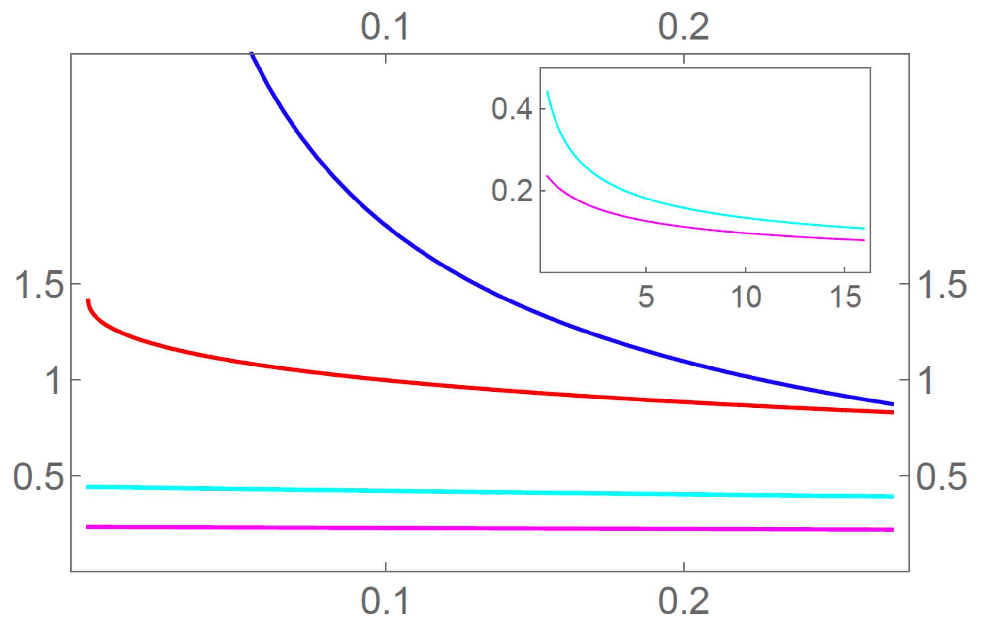
As shown in [37], the Birman–Schwinger operator B E , E < 1 2 , with integral kernel (4) is Hilbert–Schmidt (H-S) with H-S norm bounded by:
1 8 π ( 1 2 E ) 3 2 + 1 1 2 E 2 + 1 4 π 3 ( 3 2 E ) 3 .
As a consequence, the modified Fredholm determinant will have to be used in order to determine the eigenvalues of H λ , that is to say those values of E for which
det 2 1 λ B E = 0 .
We remind the reader that the latter determinant is defined by the formula (see [1,47,48])
det 2 1 + A = det 1 + A e Tr ( A ) , A T 2 ,
where det denotes the ordinary Fredholm determinant (see [1,49]) and T 2 is the H-S class.
By noting that γ n ( E ) = 2 ( n + 1 2 E ) 0 as E n + 1 2 from below for any n; then, for any E in the left neighbourhood of n + 1 2 , it should be possible to write λ B E as the sum of a rank one operator, which is divergent as E n + 1 2 , and a Hilbert–Schmidt operator, which remains bounded as E n + 1 2 . This is a consequence of some standard techniques developed by Simon and Klaus [50] in the seventies.
Let us see how this works for n = 0 , that is to say near E 0 = 1 2 , the ground state energy of the unperturbed harmonic oscillator. To this end, let us set E 0 ( λ ) = 1 2 ϵ 0 , so that γ 0 ( ϵ 0 ) = 2 ϵ 0 , and:
B ϵ 0 = P ϵ 0 + M ϵ 0 + N ϵ 0 ,
where P ϵ 0 is the rank one operator with integral kernel equal to
P ϵ 0 ( x , x , y , y ) = e x 2 / 2 ϕ 0 ( x ) e x 2 / 2 ϕ 0 ( x ) e y 2 / 2 e 2 ϵ 0 y e y 2 / 2 e 2 ϵ 0 y 2 ϵ 0 ,
M ϵ 0 is the trace class operator with integral kernel equal to
M ϵ 0 ( x , x , y , y ) = e x 2 / 2 ϕ 0 ( x ) e x 2 / 2 ϕ 0 ( x ) e y 2 / 2 e 2 ϵ 0 y y e y 2 / 2 2 ϵ 0 P ϵ 0 ( x , x , y , y ) ,
and N ϵ 0 is the positive Hilbert–Schmidt operator with integral kernel equal to
N ϵ 0 ( x , x , y , y ) = e ( x 2 + y 2 ) 2 n = 1 e γ n ( ϵ 0 ) y y γ n ( ϵ 0 ) ϕ n ( x ) ϕ n ( x ) e ( x 2 + y 2 ) 2 ,
with γ n ( ϵ 0 ) = 2 n + ϵ 0 , n 1 .
The rank one operator P ϵ 0 is clearly divergent as ϵ 0 0 + . As will be shown in the mathematical appendix, the operator N ϵ 0 converges in the H-S norm to the positive H-S operator with integral kernel given by the function
N 0 ( x , x , y , y ) = e ( x 2 + y 2 ) 2 n = 1 e 2 n y y 2 n ϕ n ( x ) ϕ n ( x ) e ( x 2 + y 2 ) 2 .
Although it is slightly more challenging from the mathematical point of view, it can also be shown (see Appendix A) that M ϵ 0 M 0 in the trace class norm, where M 0 is the trace class operator with integral kernel equal to:
M 0 ( x , x , y , y ) = e x 2 / 2 ϕ 0 ( x ) e x 2 / 2 ϕ 0 ( x ) e y 2 / 2 y + y y y e y 2 / 2 .
Therefore, (10) can be written as:
det 2 1 λ P ϵ 0 + M ϵ 0 + N ϵ 0 = 0 ,
which, taking into account that 1 λ M ϵ 0 + N ϵ 0 is invertible for small values of λ in a suitable right neighbourhood of ϵ 0 = 0 due to the results of Theorems A2 and A3 in Appendix A, can be recast as:
det 2 1 λ M ϵ 0 + N ϵ 0 det 2 1 λ P ϵ 0 1 λ M ϵ 0 + N ϵ 0 1 = 0 ,
Given that the first determinant cannot vanish for small values of λ in a suitable right neighbourhood of ϵ 0 = 0 , we need only seek the roots of
det 2 1 λ P ϵ 0 1 λ M ϵ 0 + N ϵ 0 1 = 0 ,
which, taking into account that P ϵ 0 T 1 since it is a rank one operator, can be written as (see [1,47]):
det 1 λ P ϵ 0 1 λ M ϵ 0 + N ϵ 0 1 e λ · tr P ϵ 0 1 λ M ϵ 0 + N ϵ 0 1 = 0 .
As the second factor cannot vanish, the equation determining the energy of the ground state reduces to:
det 1 λ P ϵ 0 1 λ M ϵ 0 + N ϵ 0 1 = 0 ,
involving only a Fredholm determinant. Furthermore, since P ϵ 0 is a rank one operator, (21) becomes:
1 λ · tr P ϵ 0 1 λ M ϵ 0 + N ϵ 0 1 = 0 ,
which explicitly reads:
2 ϵ 0 = λ e x 2 / 2 ϕ 0 ( x ) e y 2 / 2 2 ϵ 0 y × S ( x , x , y , y ) e x 2 / 2 ϕ 0 ( x ) e y 2 / 2 2 ϵ 0 y d x d x d y d y ,
S ( x , x , y , y ) being the integral kernel of the operator 1 λ M ϵ 0 + N ϵ 0 1 .
By mimicking the argument used in [49] essentially based on the implicit function theorem, we can prove the existence and the analyticity of the unique solution γ 0 ( λ ) = 2 ϵ 0 ( λ ) near λ = 0 , γ 0 = 0 . In order to approximate the solution with satisfactory accuracy, it makes sense to have e y 2 / 2 2 ϵ 0 y replaced by e y 2 / 2 and 1 λ M ϵ 0 + N ϵ 0 1 replaced by its linearisation evaluated at ϵ 0 = 0 , that is to say 1 + λ M 0 + N 0 , so that the resulting equation reads:
2 ϵ 0 = λ e x 2 ϕ 0 2 ( x ) d x 2 e y 2 d y 2 + λ 2 e x 2 / 2 ϕ 0 ( x ) e y 2 / 2 M 0 ( x , x , y , y ) e x 2 / 2 ϕ 0 ( x ) e y 2 / 2 d x d x d y d y + λ 2 e x 2 / 2 ϕ 0 ( x ) e y 2 / 2 N 0 ( x , x , y , y ) e x 2 / 2 ϕ 0 ( x ) e y 2 / 2 d x d x d y d y .
The calculation of the first summand on the right hand side of (24) is quite straightforward:
I 1 = λ e x 2 ϕ 0 2 ( x ) d x 2 e y 2 d y 2 = λ π e 2 x 2 d x 2 e y 2 d y 2 = π λ 2 .
Let us evaluate the second term on the right hand side of (24), using the form of the integral kernel M 0 ( x , x , y , y ) given in (16)
I 2 = λ 2 e x 2 ϕ 0 2 ( x ) d x 2 e y 2 y 2 y + y y y d y d y ,
whose value turns out to be
I 2 = 1 2 ( 2 2 ) π λ 2 .
Finally, let us now focus on the evaluation of the last summand on the right hand side of (24) using the form of the integral kernel N 0 ( x , x , y , y ) given in (15), that is to say:
I 3 = λ 2 m = 1 1 2 m ϕ 0 ( x ) e x 2 ϕ m ( x ) d x 2 e y 2 e 2 m y y e y 2 d y d y = π λ 2 m = 1 1 2 m ϕ 0 3 ( x ) ϕ 2 m ( x ) d x 2 e y 2 e 2 m y y e y 2 d y d y .
As shown in [34],
( ϕ 0 , ϕ 0 2 ϕ 2 m ) 2 = ϕ 2 m 2 ( 0 ) 2 2 m + 1 π ,
so that (27) becomes:
I 3 = π λ 2 4 m = 1 ϕ 2 m 2 ( 0 ) 2 2 m m e y 2 e 2 m y y e y 2 d y d y .
As a consequence of Schwarz inequality, we get that the double integral in (28) is bounded by:
I 3 π λ 2 4 m = 1 ϕ 2 m 2 ( 0 ) 2 2 m m e 2 y 2 d y 1 / 2 e 2 m y y e y 2 d y 2 d y 1 / 2 < π λ 2 4 m = 1 ϕ 2 m 2 ( 0 ) 2 2 m m e 2 y 2 d y e 2 m y d y = π λ 2 4 2 m = 1 ϕ 2 m 2 ( 0 ) 2 2 m m < ,
as follows by using Young’s inequality to estimate the convolution, that is to say
f g 2 f 1 g 2 ,
with f ( x ) = e 2 m x and g ( x ) = e x 2 .
It is worth stressing that the fast convergence of the series defining I 3 is ensured by the fact that the m-th term of the dominating series behaves like m 3 2 2 2 m , due to the explicit expression of the harmonic oscillator eigenfunctions evaluated at 0 (see [45,46]).
Having shown the convergence of the series (28), we rewrite it as:
I 3 = π λ 2 8 m = 1 ϕ 2 m 2 ( 0 ) 2 2 m m e m e y 2 [ e 2 m y erfc ( m + y ) + e 2 m y erfc ( m y ) ] d y = π λ 2 8 S ,
which defines S . The almost straightforward estimate
m = 11 ϕ 2 m 2 ( 0 ) 2 2 m m e y 2 e 2 m y y e y 2 d y d y π 2 m = 11 ϕ 2 m 2 ( 0 ) 2 2 m m π 2 ϕ 22 2 ( 0 ) 11 m = 11 1 2 2 m = π 2 ϕ 22 2 ( 0 ) 11 · 2 22 m = 0 1 2 2 m = π 2 ϕ 22 2 ( 0 ) 33 2 20 ,
whose approximate value is given by 3.780591 × 10 8 , shows that the difference S S 10 is of the order 10 8 , so that a fairly accurate approximation of S is given by the sum of the first ten terms in the series in (29), let us denote the sum of these terms by S 10 = 0.09397 . Consequently, I 3 0.03690 λ 2 . Incidentally, it is worth noting that the latter contribution to the quadratic term is far smaller than the one from the second summand, namely I 2 = 1 2 ( 2 2 ) π λ 2 0.51914 λ 2 . Hence, the quadratic term in λ is accurately approximated by I 2 + I 3 0.55604 λ 2 .
Summarising the previous results, we have that the expansion of 2 ϵ 0 up to the second order of the coupling constant is given by (24):
2 ϵ 0 ( λ ) = π λ 2 + 1 2 ( 2 2 ) π + π 8 S λ 2 ,
so that
ϵ 0 ( λ ) = π λ 2 8 π + 2 2 + π 4 S λ 2 ,
which finally leads to the desired expansion for the ground state energy:
E 0 ( λ ) = 1 2 ϵ 0 ( λ ) = 1 2 π λ 2 8 π + 2 2 + π 4 S λ 2 .
The plot of the latter expansion is shown in Figure 1.
Before closing this section, we wish to provide the reader with some detailed information regarding the magnitudes of the norms of the relevant operators. This quantitative information will be crucial if one wishes to grasp the structure of the eigenvalues above the energy of the ground state. Let us start by recalling that
P ϵ 0 = P ϵ 0 1 = 1 2 ϵ 0 e x 2 ϕ 0 2 ( x ) d x e y 2 2 2 ϵ 0 y d y = π ϵ 0 e 2 ϵ 0 erfc ( 2 ϵ 0 ) 2 ,
which clearly diverges as ϵ 0 0 from above, thus ensuring the existence of the ground state regardless of the smallness of the coupling constant.
Next, as shown in the mathematical appendix, we have:
M ϵ 0 1 = e x 2 ϕ 0 2 ( x ) d x 1 e 2 γ 0 ( ϵ 0 ) y γ 0 ( ϵ 0 ) e y 2 d y = π ϵ 0 1 e 2 ϵ 0 erfc ( 2 ϵ 0 ) 2 M 0 1 = 2 ,
as ϵ 0 0 from above. Another easy consequence of Theorem A3 in Appendix A is that
N ϵ 0 2 N 0 2 < 1.3 < 2 ,
which clearly implies that the eigenvalues of the Hamiltonian H λ arising from the presence of N ϵ 0 are bound to occur for larger values of λ than those arising from the presence of M ϵ 0 in the modified Fredholm determinant. Furthermore, as follows from Theorem A1 in Appendix A, for any n 1 , we get:
K ϵ 0 , n 1 = π 2 n + ϵ 0 ϕ 2 n 2 ( 0 ) π 2 n ϕ 2 n 2 ( 0 ) = K 0 , n 1 .
In particular, we have:
K ϵ 0 , 1 1 = π 2 1 + ϵ 0 ϕ 2 2 ( 0 ) π 2 ϕ 2 2 ( 0 ) = π 4 = K 0 , 1 1 0.44311 ,
and
K ϵ 0 , 2 1 = π 2 2 + ϵ 0 ϕ 4 2 ( 0 ) π 2 2 ϕ 4 2 ( 0 ) = 3 π 16 2 = K 0 , 2 1 0.23500 ,
which imply that the eigenvalues of H λ arising from K ϵ 0 , 1 and K ϵ 0 , 2 are bound to emerge for larger values of λ than those arising M ϵ 0 . The information resulting from (34), (35), (38), (39) is depicted in Figure 2.

4. Final Remarks

Two-dimensional quantum models are of increasing interest in mathematical physics due to a wide range of applications. Solving the eigenvalue problem for the Schrödinger equation with some particularly interesting confinement potentials in two dimensions often gives rise to complicated mathematical problems, mainly because of the logarithmic singularity of the two-dimensional Green function at the origin. The system under study in the present article, as described in Section 2, is a typical example thereof. Here, even the estimation of the energy value of the ground state is far from trivial and requires advanced mathematical tools. As a matter of fact, even the study of a model with a sharply peaked impurity such as the Gaussian one becomes more complicated if the dimension changes from one to two, as a consequence of the fact that, while the Birman–Schwinger operator is trace class in one dimension, it is only Hilbert–Schmidt in two dimensions. This modification implies that the modified Fredholm determinant will have to be used in place of the ordinary Fredholm determinant in order to study the eigenvalues created by the impurity.
In a previous paper by ourselves, a lower bound for the energy spectrum of the model under consideration in the present manuscript has been found. To that end, we have already made use of sophisticated mathematical tools, first to prove the self-adjointness of the Hamiltonian and then using the properties of the Birmann–Schwinger operator to draw our conclusions. Now, we went further and have been able to find the approximate value of the energy of the ground state, using similar functional analytic methods.
Furthermore, it is conceptually possible to determine, up to some degree of accuracy, at least the first excited state. However, this task will require additional mathematical work and even more complex calculations, so that we have decided to put off this analysis until a forthcoming paper.

Author Contributions

Conceptualization, S.F.; Formal analysis, M.G. and F.R.; Funding acquisition, L.M.N.; Investigation, S.F., L.M.N. and F.R.; Methodology, S.F. and F.R.; Project administration, L.M.N.; Supervision, L.M.N.; Writing—original draft, S.F., M.G. and F.R.; Writing—review and editing, M.G. and L.M.N. All authors listed have made a substantial, direct, and intellectual contribution to the work. All authors have read and agreed to the published version of the manuscript.

Funding

This research was funded by Junta de Castilla y León and FEDER, Project BU229P18.

Data Availability Statement

Not applicable.

Conflicts of Interest

The authors declare no conflict of interest.

Appendix A. Some Mathematical Results

In this appendix we rigorously prove three mathematical results used throughout our paper.

Appendix A.1. First Theorem

First of all, we are going to demonstrate a result relative to the integral kernel introduced in Equation (4).
Theorem A1.
The function
K E , n ( x , x , y , y ) = ϕ n ( x ) e ( x 2 + y 2 ) 2 e γ n ( E ) y y γ n ( E ) ϕ n ( x ) e ( x 2 + y 2 ) 2 , γ n ( E ) = 2 n + 1 2 E , E < 1 2 ,
defines the integral kernel of a positive trace class operator for any integer n 0 .
Proof. 
It is immediate to notice that the function is continuous and
K E , n ( x , x , y , y ) = 1 γ n ( E ) ϕ n 2 ( x ) e ( x 2 + y 2 ) 0 ,
for any n 0 , E < 1 2 . Furthermore, for any n 0 , E < 1 2 ,
K E , n ( x , x , y , y ) d x d y = 1 γ n ( E ) ϕ n 2 ( x ) e ( x 2 + y 2 ) d x d y = π γ n ( E ) e x 2 ϕ n 2 ( x ) d x = π γ n ( E ) ( ϕ n , ϕ 0 2 ϕ n ) = π 2 γ n ( E ) ϕ 2 n 2 ( 0 ) < ,
the last equality being due to [35,44]. Hence, due to (A2) and (A3), K E , n ( x , x , y , y ) meets both requirements of the Lemma listed after Theor. XI.31 in [51] by invoking which we can claim that the function is actually the integral kernel of a positive trace class operator whose trace is exactly equal to the right hand side of (A3). □

Appendix A.2. Second Theorem

The second result we wish to prove in this mathematical appendix is the anticipated convergence of the trace class operator M ϵ 0 with integral kernel given by (13) to the trace class operator M 0 with integral kernel given by (16).
The proof essentially mimics the one of Theorem 3.1 in [52] (see also [21]). It is worth mentioning that a similar result also holds in the case of the resolvent of the one-dimensional Dirac Hamiltonian (see [53]).
Theorem A2.
The operator M ϵ 0 with integral kernel given by (13) is trace class and converges to the trace class operator M 0 with integral kernel given by (16) in the norm topology of trace class operators.
Proof. 
As an immediate consequence of the previous theorem, it is clear that the first summand on the right hand side of (13) is the integral kernel of a trace class operator, so that M ϵ 0 ( λ ) , being given by a linear combination of a trace class operator and a rank one operator, is trace class as well.
Before proving the stated convergence, let us show that the limiting operator M 0 is trace class. Its integral kernel is clearly continuous and, as an easy consequence of the triangular inequality, we have:
M 0 ( x , x , y , y ) = e x 2 / 2 ϕ 0 ( x ) e x 2 / 2 ϕ 0 ( x ) e y 2 / 2 y + y y y e y 2 / 2 0 .
Furthermore,
M 0 ( x , x , y , y ) = 2 e x 2 ϕ 0 2 ( x ) y e y 2 0 ,
and
R 2 M 0 ( x , x , y , y ) d x d y = 2 R 2 e x 2 ϕ 0 2 ( x ) y e y 2 d x d y = 2 e x 2 ϕ 0 2 ( x ) d x 0 2 y e y 2 d y = 2 π e 2 x 2 d x 0 e s d s = 2 π e s 2 d s = 2 .
Therefore, by invoking again the aforementioned Lemma in [51], the function M 0 ( x , x , y , y ) is the kernel of a positive trace class operator M 0 with trace equal to
M 0 ( x , x , y , y ) d x d y = 2 .
Let us focus now on the proof of the stated convergence. Given that, as γ 0 ( ϵ 0 ) = 2 ϵ 0 0 + ,
e γ 0 ( ϵ 0 ) | y y | e γ 0 ( ϵ 0 ) | y | + | y | γ 0 ( ϵ 0 ) | y | + | y | | y y | = 2 min ( | y | , | y | ) 0 ,
we immediately get the pointwise convergence of the integral kernel, that is to say
M ϵ 0 ( x , x , y , y ) M 0 ( x , x , y , y )
as γ 0 ( ϵ 0 ) = 2 ϵ 0 0 + , which, in turn, implies the weak convergence of M ϵ 0 to M 0 . Furthermore, as γ 0 ( ϵ 0 ) = 2 ϵ 0 0 + ,
M ϵ 0 ( x , x , y , y ) d x d y = e x 2 ϕ 0 2 ( x ) d x 1 e 2 γ 0 ( ϵ 0 ) y γ 0 ( ϵ 0 ) e y 2 d y 2 e x 2 ϕ 0 2 ( x ) d x y e y 2 d y = 2 = M 0 ( x , x , y , y ) d x d y ,
which is equivalent to saying that the trace class norm of M ϵ 0 converges to that of M 0 as γ 0 ( ϵ 0 ) = 2 ϵ 0 0 + . As a result of a well-known theorem on the convergence of sequences of operators belonging to the trace class ideal (Ref. [41] Theorem 2.21), the latter convergence, together with the weak convergence of M ϵ 0 to M 0 , implies the convergence in the trace class norm, which completes our proof of the theorem.  □

Appendix A.3. Third Theorem

The last result that we are going to demonstrate refers to the operator N ϵ 0 , introduced in (14) through an integral kernel.
Theorem A3.
The operator N ϵ 0 with integral kernel given by (14) is Hilbert–Schmidt and converges to the H-S operator N 0 with integral kernel given by (15) in the norm topology of H-S operators.
Proof. 
As follows from Theorem A1, each summand in both N ϵ 0 and N 0 is trace class. However, as shown in (8), both infinite sums do not belong to T 1 . They belong instead to T 2 as a consequence of an easy modification (removal of the first summand) of the proof of Theorem 2.1 in [37]. For their H-S norms, given by
tr ( N ϵ 0 2 ) = N ϵ 0 2 x , x , y , y d x d y = m = 1 n = 1 ϕ m , e ( · ) 2 ϕ n 2 R 2 e y 2 e 2 ( m + ϵ 0 ) + 2 ( n + ϵ 0 ) y y 2 ( m + ϵ 0 ) ( n + ϵ 0 ) e y 2 d y d y
and
tr ( N 0 2 ) = N 0 2 x , x , y , y d x d y = m = 1 n = 1 ϕ m , e ( · ) 2 ϕ n 2 e y 2 e ( 2 m + 2 n ) y y 2 m n e y 2 d y d y ,
we have by using first Young’s inequality to estimate the convolution and later Schwartz inequality:
tr ( N ϵ 0 2 ) tr ( N 0 2 ) π 3 2 2 m = 1 n = 1 ϕ m , ϕ 0 2 ϕ n 2 m 3 4 n 3 4 π 3 2 2 n = 1 | | ϕ 0 ϕ n | | 2 2 n 3 4 2 = = π 3 2 2 n = 1 ϕ n , ϕ 0 2 ϕ n n 3 4 2 = π 3 2 4 n = 1 ϕ 2 n 2 ( 0 ) n 3 4 2 1.66265 ,
the convergence of the series inside the square brackets being ensured by the fact that ϕ 2 n 2 ( 0 ) / n 3 4 decays like n 5 / 4 . Therefore, by dominated convergence:
tr ( N ϵ 0 2 ) = N ϵ 0 2 x , x , y , y d x d y N 0 2 x , x , y , y d x d y = tr ( N 0 2 )
as ϵ 0 0 + . By invoking again Theorem 2.21 in [41], it follows that (A13) and the weak convergence of N ϵ 0 to N 0 imply that the convergence actually takes place in the H-S norm. □

References

  1. Albeverio, S.; Gesztesy, F.; Høegh-Krohn, R.; Holden, H. Solvable Models in Quantum Mechanics, 2nd ed.; AMS Chelsea Series; AMS Chelsea: Providence, RI, USA, 2004. [Google Scholar]
  2. Albeverio, S.; Kurasov, P. Singular Perturbations of Differential Operators; Cambridge UP: Cambridge, UK, 1999. [Google Scholar]
  3. Seba, P. Some remarks on the δ-interaction in one dimension. Czechoslov. J. Phys. 1986, 36, 667–673. [Google Scholar] [CrossRef]
  4. Bräunlich, G.; Hainzl, C.; Seiringer, R. On contact interactions as limits of short-range potentials. Met. Funct. Anal. Top. 2013, 19, 364–375. [Google Scholar]
  5. Bohm, A. Quantum Mechanics. Foundations and Applications; Springer: New York, NY, USA, 1994. [Google Scholar]
  6. Kurasov, P. Distribution theory for discontinuous test functions and differential operators with generalized coefficients. J. Math. Anal. Appl. 1996, 201, 297–323. [Google Scholar] [CrossRef] [Green Version]
  7. Albeverio, S.; Kurasov, P. Pseudo-differential operators with point interactions. Lett. Math. Phys. 1997, 41, 79–92. [Google Scholar] [CrossRef]
  8. Albeverio, S.; Fassari, S.; Rinaldi, F. The discrete spectrum of the spinless onedimensional Salpeter Hamiltonian perturbed by δ-interactions. J. Phys. A Math. Theor. 2015, 48, 185301. [Google Scholar] [CrossRef]
  9. Erman, F.; Gadella, M.; Uncu, H. One-dimensional semirelativistic Hamiltonian with multiple Dirac delta potentials. Phys. Rev. D 2017, 95, 045004. [Google Scholar] [CrossRef] [Green Version]
  10. Muñoz-Castañeda, J.M.; Nieto, L.M.; Romaniega, C. Hyperspherical δ-δ potentials. Ann. Phys. 2019, 400, 246–261. [Google Scholar] [CrossRef] [Green Version]
  11. Antonie, J.P.; Gesztesy, F.; Shabani, J. Exactly solvable models of sphere interaction in quantum mechanics. J. Phys. A Math. Gen. 1987, 20, 3687–3712. [Google Scholar] [CrossRef]
  12. Nyeo, S.-L. Regularization methods for delta-function potential in two-dimensional quantum mechanics. Am. J. Phys. 2000, 68, 571–575. [Google Scholar] [CrossRef] [Green Version]
  13. Jackiw, R. Diverse Topics in Mathematical Physics; Word Scientific: Singapore, 1995; pp. 41–48. [Google Scholar]
  14. Goszdinsky, P.; Tarrach, R. Learning Quantum Field Theory from elementary quantum mechanics. Am. J. Phys. 1991, 59, 70–74. [Google Scholar] [CrossRef]
  15. Erman, F.; Uncu, H. Green’s function formulation of multiple nonlinear Dirac delta-function potential in one dimension. Phys. Lett. A 2020, 384, 126227. [Google Scholar] [CrossRef] [Green Version]
  16. Fassari, S.; Popov, I.; Rinaldi, F. On the behaviour of the two-dimensional Hamiltonian −Δ + λ[δ( x + x 0 ) + δ( x x 0 )] as the distance between the two centers vanishes. Phys. Scr. 2020, 95, 075209. [Google Scholar] [CrossRef]
  17. Klaus, M. A remark about weakly coupled one-dimensional Schrödinger operators. Helv. Phys. Acta 1979, 52, 223–229. [Google Scholar]
  18. Klaus, M. Some applications of the Birman-Schwinger principle. Helv. Phys. Acta 1982, 55, 49–68. [Google Scholar]
  19. Fassari, S. An estimate regarding one-dimensional point interactions. Helv. Phys. Acta 1995, 68, 121–125. [Google Scholar]
  20. Holden, H. On coupling constant thresholds in two dimensions. J. Oper. Theory 1985, 14, 263–276. [Google Scholar]
  21. Fassari, S.; Klaus, M. Coupling constant thresholds of perturbed periodic Hamiltonians. J. Math. Phys. 1998, 39, 4369–4416. [Google Scholar] [CrossRef] [Green Version]
  22. Fassari, S.; Gadella, M.; Glasser, M.L.; Nieto, L.M. Rinaldi, F. Level crossings of eigenvalues of the Schrödinger Hamiltonian of the isotropic harmonic oscillator perturbed by a central point interaction in different dimensions. Nanosyst. Phys. Chem. Math. 2018, 9, 179–186. [Google Scholar] [CrossRef]
  23. Fassari, S.; Inglese, G. Spectroscopy of a three-dimensional isotropic harmonic oscillator with a δ-type perturbation. Helv. Phys. Acta 1996, 69, 130–140. [Google Scholar]
  24. Albeverio, S.; Fassari, S.; Rinaldi, F. Spectral properties of a symmetric three-dimensional quantum dot with a pair of identical attractive δ-impurities symmetrically situated around the origin. Nanosyst. Phys. Chem. Math. 2016, 7, 268–289. [Google Scholar] [CrossRef] [Green Version]
  25. Albeverio, S.; Fassari, S.; Rinaldi, F. Spectral properties of a symmetric three-dimensional quantum dot with a pair of identical attractive δ-impurities symmetrically situated around the origin II. Nanosyst. Phys. Chem. Math. 2016, 7, 803–815. [Google Scholar] [CrossRef] [Green Version]
  26. Albeverio, S.; Fassari, S.; Rinaldi, F. A remarkable spectral feature of the Schrödinger Hamiltonian of the harmonic oscillator perturbed by an attractive δ-interaction centred at the origin: Double degeneracy and level crossings. J. Phys. A Math. Theor. 2013, 46, 385305. [Google Scholar] [CrossRef]
  27. Fassari, S.; Gadella, M.; Glasser, M.L.; Nieto, L.M. Spectroscopy of a one-dimensional V-shaped quantum well with a point impurity. Ann. Phys. 2018, 389, 48–62. [Google Scholar] [CrossRef] [Green Version]
  28. Fassari, S.; Gadella, M.; Nieto, L.M.; Rinaldi, F. Spectral properties of the 2D Schrödinger Hamiltonian with various solvable confinements in the presence of a central point perturbation. Phys. Scr. 2019, 94, 055202. [Google Scholar] [CrossRef] [Green Version]
  29. Sasaki, R.; Znojil, M. One-dimensional Schrödinger equation with non-analytic potential V(x) = −g2exp(−|x|) and its exact Bessel-function solvability. J. Phys. A Math. Theor. 2016, 49, 445303. [Google Scholar] [CrossRef] [Green Version]
  30. Fassari, S.; Gadella, M.; Nieto, L.M.; Rinaldi, F. On the spectrum of the 1D Schrödinger Hamiltonian perturbed by an attractive Gaussian potential. Acta Polytech. 2017, 57, 385–390. [Google Scholar] [CrossRef] [Green Version]
  31. Muchatibaya, G.; Fassari, S.; Rinaldi, F.; Mushanyu, J. A note on the discrete spectrum of Gaussian wells (I): The ground state energy in one dimension. Adv. Math. Phys. 2016, 2016, 2125769. [Google Scholar] [CrossRef] [Green Version]
  32. Fernández, F.M. Quantum Gaussian wells and barriers. Am. J. Phys. 2011, 79, 752–754. [Google Scholar] [CrossRef]
  33. Nandi, S. The quantum Gaussian well. Am. J. Phys. 2010, 78, 1341–1345. [Google Scholar] [CrossRef] [Green Version]
  34. Fassari, S.; Nieto, L.M.; Rinaldi, F. The two lowest eigenvalues of the harmonic oscillator in the presence of a Gaussian perturbation. Eur. Phys. J. Plus 2020, 135, 728. [Google Scholar] [CrossRef]
  35. Fassari, S.; Rinaldi, F. Exact calculation of the trace of the Birman-Schwinger operator of the one-dimensional harmonic oscillator perturbed by an attractive Gaussian potential. Nanosyst. Phys. Chem. Math. 2019, 10, 608–615. [Google Scholar] [CrossRef] [Green Version]
  36. Harrison, P. Quantum Wells, Wires, Dots; Wiley: Chichester, UK, 2009. [Google Scholar]
  37. Albeverio, S.; Fassari, S.; Gadella, M.; Nieto, L.M.; Rinaldi, F. The Birman-Schwinger operator for a parabolic quantum well in a zero-thickness layer in the presence of a two-dimensional attractive Gaussian impurity. Front. Phys. 2019, 7, 102. [Google Scholar] [CrossRef] [Green Version]
  38. Reed, M.; Simon, B. Fourier Analysis, Self-Adjointness, Methods in Modern Mathematical Physics; Academic Press: New York, NY, USA, 1975. [Google Scholar]
  39. Duclos, P.; Štovicek, P.; Tušek, M. On the two-dimensional Coulomb-like potential with a central point interaction. J. Phys. A Math. Theor. 2010, 43, 474020. [Google Scholar] [CrossRef] [Green Version]
  40. Reed, M.; Simon, B. Functional Analysis, Methods in Modern Mathematical Physics; Academic Press: New York, NY, USA, 1972. [Google Scholar]
  41. Simon, B. Trace Ideals and Their Applications; Cambridge University Press: Cambridge, UK, 1979. [Google Scholar]
  42. Arfken, G.B. Mathematical Methods for Physicists, 3rd ed.; Academic Press: New York, NY, USA, 1985. [Google Scholar]
  43. Correggi, M.; Dell’Antonio, G.; Finco, D. Spectral analysis of a two-body problem with zero-range perturbation. J. Funct. Anal. 2008, 255, 502–531. [Google Scholar] [CrossRef] [Green Version]
  44. Wang, W.-M. Pure Point Spectrum of the Floquet Hamiltonian for the Quantum Harmonic Oscillator Under Time Quasi-Periodic Perturbations. Commun. Math. Phys. 2008, 277, 459–496. [Google Scholar] [CrossRef]
  45. Fassari, S.; Inglese, G. On the spectrum of the harmonic oscillator with a δ-type perturbation. Helv. Phys. Acta 1994, 67, 650–659. [Google Scholar]
  46. Mityagin, B.S.; Siegl, P. Root system of singular perturbations of the harmonic oscillator type operators. Lett. Math. Phys. 2016, 106, 147–167. [Google Scholar] [CrossRef] [Green Version]
  47. Simon, B. The bound state of weakly coupled Schrödinger operators in one and two dimensions. Ann. Phys. 1976, 97, 279–288. [Google Scholar] [CrossRef]
  48. Gesztesy, F.; Kirsten, K. On traces and modified Fredholm determinants for half-line Schrödinger operators with purely discrete spectra. Q. Appl. Math. 2019, 77, 615–630. [Google Scholar] [CrossRef] [Green Version]
  49. Reed, M.; Simon, B. Analysis of Operators, Methods in Modern Mathematical Physics; Academic Press: New York, NY, USA, 1978. [Google Scholar]
  50. Klaus, M.; Simon, B. Coupling constant thresholds in nonrelativistic quantum mechanics. I. Short-range two-body case. Ann. Phys. 1980, 130, 251–281. [Google Scholar] [CrossRef]
  51. Reed, M.; Simon, B. Scattering Theory, Methods in Modern Mathematical Physics; Academic Press: New York, NY, USA, 1979. [Google Scholar]
  52. Fassari, S. On the bound states of non-relativistic Kronig-Penney Hamiltonians with short range impurities. Helv. Phys. Acta 1990, 63, 849–883. [Google Scholar]
  53. Fassari, S. On the bound states of relativistic Kronig-Penney Hamiltonians with short range impurities. Helv. Phys. Acta 1990, 63, 884–907. [Google Scholar]
Figure 1. Plot of the ground state energy E 0 ( λ ) as a function of λ , given in (33).
Symmetry 13 01561 g001
Figure 2. Plot of the energy dependence of the norms of the following four operators: P ϵ 0 in (34) (blue curve), M ϵ 0 in (35) (red curve), K ϵ 0 , 1 in (38), (cyan curve) and K ϵ 0 , 2 in (39) (magenta curve). In the inset, we can see more details of the two lowest curves.
Symmetry 13 01561 g002
Publisher’s Note: MDPI stays neutral with regard to jurisdictional claims in published maps and institutional affiliations.

