Search of the Shortest Path in a Communication Network with Fuzzy Cost Functions

Abstract

A communication network management system takes the measurements of its state variables at specific instants of time, considering them constant in the interval between two consecutive measurements. Nevertheless, this assumption is not true, since these variables evolve in real time. Therefore, uncertainty is inherent in the processing of the measurements during the intervals so that they cannot be efficiently managed using crisp variables. In this paper, we face this problem by modeling the communications network as a type-V fuzzy graph, where both the nodes and the links are described with precision, but the cost of each link is modeled as a triangular fuzzy number. Different fuzzy cost allocation functions and fuzzy optimization strategies are described and applied to the search for the shortest path between two nodes. An experimental study has been conducted using two representative networks: the backbone network of Nippon Telegraph and Telephone Corporation (NTT) and the National Science Foundation’s Network (NFSNET). In these networks, our fuzzy cost functions and strategies have been compared with the well-known crisp equivalents. The optimal search strategies are based on the proposed Fuzzy Dijkstra Algorithm (FDA), which is described deeply. The simulation results demonstrate that in all cases the fuzzy alternatives surpass or equal the crisp equivalents with statistically significant values. Specifically, the so-called Strategy 8 presents the best throughput, as it significantly exceeds the performance of all those evaluated, achieving a Global Mean Delivery Rate (GMDR) close to 1.

1. Introduction

The management of a communication network is mainly oriented to maximize the ratio between sent and received information for any pair of source-destination nodes while reducing transmission delays. This objective is especially relevant in high occupancy conditions. Necessary resources to achieve this objective are algorithms and routing protocols, which seek to provide the optimal path between any pair of source-destination nodes. To evaluate the goodness level of a path, it is crucial to know the state of the network by assigning a cost to every link. In this way, we compute the cost of a particular path using variables such as Used Bandwidth, Residual Bandwidth (non-used bandwidth), Packet Delay (time spent in the delivery of an information packet), Packet Delivery Ratio (ratio between delivered and sent packets), Packet Loss Ratio (one minus the Package Delivery Ratio), etc. From this knowledge, we can establish the routing tables, which contain the path communicating nodes to transmit the information at each moment.

Because of the dynamic behavior of a network, and consequently, the high variability in time of its performing conditions, the usual way to work is to compute the state variables over a given time interval using measurements obtained in the immediately previous time interval. So, typical routing protocols update the state (cost) of links in two possible ways [1]:

(A)

By time intervals. Each cost value (and therefore, the routing tables) is updated with a constant periodicity. This update is either to the instantaneous state value at the beginning of the new interval or to the mean value of costs over the previous time interval.

(B)

By thresholds. Some update thresholds are fixed so that the update of a state variable is carried out when the difference between its current real value and the one determined more recently exceeds the corresponding threshold.

It is evident that, although these cost values are well defined real numbers (crisp numbers in our lingo), these procedures include a degree of uncertainty about the current state due to the fact that the variables change during a time interval. Consequently, we believe that considering this uncertainty in the decision-making process for the management should allow us to find better solutions. In this sense, some elements of Fuzzy Logic, in particular, the application of arithmetic operations and properties of fuzzy numbers, can be helpful.

As a first approach, we interpret a triangular fuzzy number as a triplet of real numbers. The numbers at the ends delimit the interval of values that can be assigned to the fuzzy number (variable values with a probability value greater than 0 in the membership function) and the central number is the value of the variable with the highest value in the membership function. This triangular fuzzy number is a particular case of the more general trapezoidal fuzzy number described in Section 3 and in [2,3]).

An essential aspect of our work is to represent the cost measurements of the network by using fuzzy numbers in order to reasonably incorporate the aforementioned uncertainty. For this objective, option (B) has an apparent advantage over option (A) as when fixing the thresholds, we are also setting the upper and lower limits of the corresponding triangular fuzzy number. However, the central value of this fuzzy number, which would theoretically be considered the most feasible one, does not have a physical justification: it would respond to an instantaneous value from which we have no information about its feasibility. Moreover, if the central value is given, we compute the upper and lower values by adding and subtracting the threshold. The crisp number corresponding to this fuzzy cost function will always be constant and equal to the central value. Therefore, the meaning of fuzzification is lost. On the other hand, option (A) does not directly provide us with the extreme values of the normalized triangular fuzzy number. However, it allows us to define them using statistical methods in such a way that we can keep the consistency with the physics of the problem and incorporating its fuzzy nature. Thus, in our case, the proposed fuzzy numbers for the time interval t are defined as follows: the central value corresponds to the mean value of the costs over the entire $t-1$ time interval, which will generate a minor error, and the extreme values correspond to the maximum and minimum values of cost measurements in the above mentioned $t-1$ time interval.

In our proposal, we model the network as a non-directed Type-V fuzzy Graph. In this type of fuzzy graph, the vertexes and the edges are physically well established, but the costs of the links are defined by a fuzzy number. In our particular case, the costs are triangular fuzzy numbers to incorporate the uncertainty [4]. Finally, the application of a fuzzy version of the Dijkstra algorithm, like the shortest path search algorithm, should give us the path between any pair of source-destination nodes with the minimum cost. This fuzzy version of Dijkstra’s algorithm can be considered as classical since it does not incorporate any consideration of uncertainty in its execution, but it incorporates uncertainty in the value of the variables (here considered as fuzzy) and in the definition of the mathematical operation between them. A very basic application of this work can be found in [5], where a pair of shortest-disjoint paths is identified with a simpler version of the Modified Dijkstra Algorithm. However, the complete description of the algorithm, the operation of the fuzzy-based costs and their comparison with other classic approaches are firstly described in a scientific journal. In particular, we now include the mathematical framework to operate with the fuzzy costs in a modified Dijkstra algorithm. In addition, the present paper defines how classical cost functions can be incorporated into the algorithm and compare them with some fuzzy-based cost functions for two illustrative network topologies. The algorithm is completely described, including the complementary procedures of the initialization phase and the relaxation of the vertexes. However, the modified Dijkstra algorithm and the preliminary operations can be found as a technical report in the repository of the University of Málaga [6].

We are also interested in highlighting the differences between this methodology, which uses fuzzy values of variables (triangular fuzzy numbers) and the so-called Fuzzy Inference (or Control) (see [7,8]), in which the measurements have precise values, but the uncertainty lies on the decision process itself.

Summarizing, the main contribution of this work is the presentation of a methodology to optimize the search for the shortest path between two nodes during the global management of a communication network. This methodology is characterized by modeling the network as a Non-directed Type-V Fuzzy Graph and applying a fuzzy Dijkstra algorithm that is adapted to operate with fuzzy numbers. To show the goodness of our approach, we have two objectives:

(i)

To show the competitiveness of the methodology based on the fuzzy model versus that based on the traditional model using crisp magnitudes. To do this, we reconstruct the currently used classical cost functions and strategies for searching the optimal path in the fuzzy model. Then, we compare both visions (classical and fuzzy) in the same experimental environment for two representative network topologies. The results show that the fuzzy model is more efficient (or equal in the worst case), being this conclusion validated by a statistical parameter.

(ii)

To illustrate that the fuzzy model allows us to define new metrics that take advantage from the experimental uncertainty above mentioned. Thus, we provide a new strategy, and its cost function (referred to as Strategy 8), which has no equivalent in the classic model and by far exceeds all the other strategies analyzed in effectiveness.

Thus, the organization of this paper is as follows: we devote Section 2 to compile some related works from the points of view of both the application in the communication environment and the use of Fuzzy Logic. In Section 3, we describe the fuzzy model of the communication network and we proceed with the definition of various types of fuzzy numbers and their possible interpretation. Section 4 introduces our proposal of Fuzzy Dijkstra Algorithm applied on a network with fuzzy costs and using the Total Integral Method proposed in [9] as the ranking procedure for fuzzy numbers. Section 5 presents the application of these theoretical concepts to a communication network with a description of the communication network used, the different cost functions used in the comparison as well as the different strategies to search the optimal path (with a particular interest in Strategy 8). Section 6 deals with our experimental study, where the reader can find the simulation results and their discussion. Finally, Section 7 summarizes the main and conclusive ideas of this work and we also outline future research lines of work.

2. Related Work

In this Section, we will first review the strategies used to search the shortest (or more efficient) path in a communication network. Concerning classic strategies (based on crisp magnitudes), we consider some approaches to be among the most known and used at the moment. The Shortest-Widest (SW) strategy presented in [10] searches for the path with the largest residual bandwidth path (that is, the more efficient path). When there are two paths with the same value for this metric, the criterion about the path length is used so that the one with the lower number of hops is selected. The Widest-Shortest (WS) strategy, explained in [11], proceeds contrary to SW. WS searches for the path with the minimum number of hops, and if there are two paths with the same number of hops, the one with the maximum residual bandwidth is selected. The Shortest Dist Path is described in [12,13]. This strategy uses a hyperbolic cost function based on the inverse of the residual bandwidth to identify the best path. In these works, the authors perform an exhaustive comparison between SW, WS and Shortest Dist Path algorithm. When there is traffic without a reserve of resources, the Shortest Dist Path algorithm is clearly advantageous, especially under overload conditions. In [14], the goal is to find the optimum path in order to reduce the Bandwidth Rejection Ratio (BRR). A comparison of cost functions applied to software-defined networks is carried out. In fact, based on a cost function that uses a variant of the Shortest Dist Path algorithm, the algorithm DORA 0.9 provides the best results in [15]. In [16], the authors carry out an extensive study of different strategies and different network topologies concluding that widest-shortest is the best strategy among the studied ones in high load conditions.

Other approaches to the optimal path search problem in a communication network are based on the adaptation of control techniques based on fuzzy inference. In this case, the values of the cost functions on the links are crisp, but the uncertainty is applied to the inference process itself. Thus, in [17], the authors developed a fuzzy inference system using the Expected Transmission Time (ETX) and the number of hops as input variables to find the best server node in a P2P wireless mesh. The fuzzification of these variables and their introduction in the fuzzy decision rules allow us to outperform the efficiency of traditional methods, which select the server node based on a min-hop or random criteria. The work in [18] addresses the problem of file sharing. The authors proposed that the server node selected for this operation is the one with the highest degree of trustworthiness. In [19], the authors proposed a fuzzy inference system to find the path in a sensor network taking into account the remaining energy, the minimum number of hops and the node traffic load. In [20], the authors addressed the problem of selecting the best communication path to reach a gateway while performing a load balancing. Fuzzy-logic functions are evaluated for this purpose. Type-II fuzzy logic has also been applied in wireless communication networks to find the optimal paths. With this technique, the work in [21] focused on selecting the best path to reach the gateway in an Internet-connected network.

An alternative fuzzy approach to the network modeling assumes that the uncertainty lies on the value of the cost functions. This uncertainty can be modeled by using fuzzy numbers. In these cases, the application of a classic path search algorithm such as Dijkstra Algorithm involves solving the problem of operating with fuzzy numbers (e.g., adding up the fuzzy costs of the links in a path) and comparing fuzzy numbers (e.g., the comparison between the total cost of two paths). In [22], the definitions of the Graded Mean Integration Representation and the expression for the sum and product of two (triangular or trapezoidal) fuzzy numbers were developed with particular mathematical rigor using an integral representation. This study allows operating and comparing fuzzy numbers. Refs. [23,24] adopted this representation, which was used to adapt the Dijkstra algorithm to fuzzy costs in a generic transportation network.

In this paper, we base our proposal on the modeling of a network by assigning a triangular fuzzy number to the links costs. For the comparison of triangular fuzzy numbers, a generalized definition for the Total Integral of a fuzzy number proposed in [9] is used. This is different from the above mentioned Graded Mean Integration Representation. The different metrics discussed above (WS, SW, Normalized Used Bandwidth) are adapted to the definition of fuzzy number and compared with the classic versions on the simulated environment of two well known communication networks, based on the topology of the Nippon Telegraph and Telephone (NTT) and the National Science Foundation’s Network (NSFNET), respectively. In general, our fuzzy versions surpass or equal the crisp versions in all cases by a small statistically significant margin. In addition, a new cost function based on the triangular fuzzy number definition is developed, and given a physical explanation of its properties. Our optimization strategy based on this latter function (named Strategy 8) surpasses the other tested algorithms, giving a result of the Delivery Bit Ratio close to 1.

Parallel to this work, this Strategy 8 has already been applied to the problem of searching for the shortest pair of disjoint edge paths in a communication network [5]. It has proven its effectiveness in managing a network with two types of traffic. This topic is of applicability in financial or governmental services, where privacy and security against external attacks are imposed requirements. On the other hand, our methodology could be transferred to city or road traffic management by modeling road or street networks as a graph where links have a limited traffic capacity that can be measured. In these conditions, actualization of traffic density cannot be carried out in a continuous time manner, thus our fuzzy modeling of the network is justified. In  [25] this problem is posed and attacked by means of methodologies based on crisp measurements.

3. Fuzzy Modeling of a Communication Network

Fuzzy graphs can be classified into five main groups according to the fuzziness of the vertex set, the edge set and/or the edge weights. For our network model, we know the vertex and the edge sets as they correspond to the nodes and the connection lines. However, the weights of the edges (the costs in our network) are fuzzy numbers, as we cannot determine their exact value. According to [4], these features lead to a Type-V fuzzy graph.

In this section, we describe the Type-V fuzzy graph associated to the network. We also provide the definition of a fuzzy number and its possible interpretation to ease a better understanding of our approach. At this point, it is necessary to clarify that the definition of a triangular fuzzy number is not equivalent to that of a triangular probability distribution. While the probability distribution responds to a binary logic (the excluded third principle is respected), the fuzzy number responds to a multivalued logic. We can say that the membership function that defines the fuzzy number does not provide the probability that the number takes a certain value, but rather the ratio in which the number is that value. Thus, processing uncertainty and the properties of both fuzzy and probabilistic approaches are different. Zimmermann distinguishes them as “linguistics” and “stochastic” uncertainty, respectively, [26,27].

Definition 1.

(Type-V fuzzy graph) A Type-V fuzzy graph is based on known vertexes and edges. However, the costs of the edges has some uncertainty. It can be interpreted as a crisp graph in which the costs of the edges are fuzzy numbers.

Our network is described as a Type-V fuzzy graph $\tilde{G}$, which is defined as follows:

• $\tilde{G}=(V,E,\mathfrak{C})$ is a triplet where,

  −

  V is the set of vertexes

  −

  E is the set of edges

  −

  $\mathfrak{C}$ is the set of fuzzy costs. ${\tilde{C}}_{ij}\in \mathfrak{C}$: fuzzy cost of edge $(i,j)$, $i,j\in V$

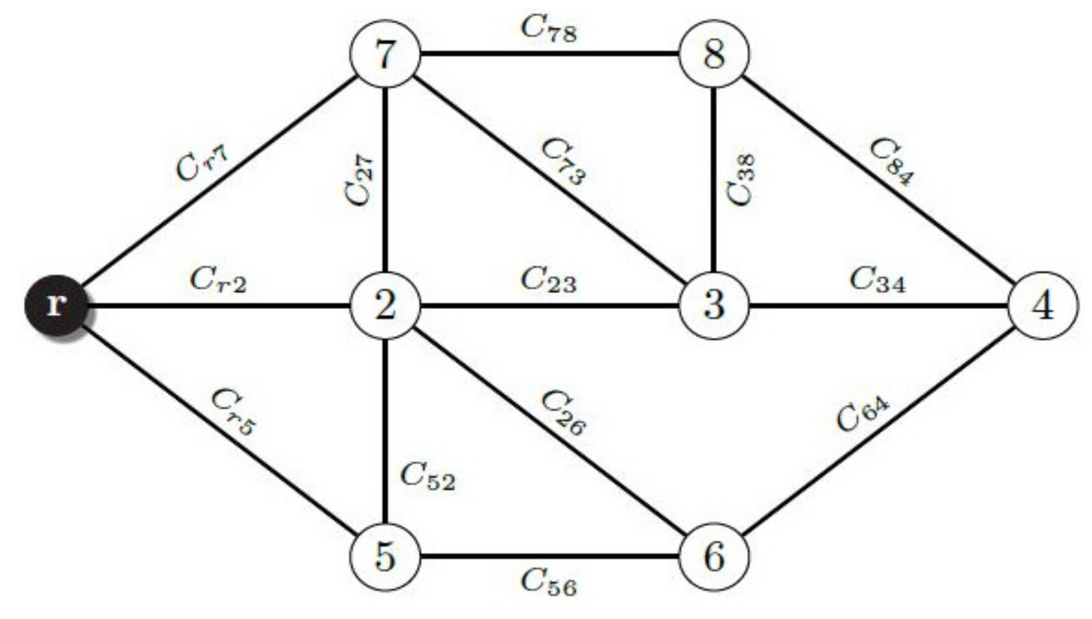
  Figure 1 depicts an example of a Type-V fuzzy graph.
• $\tilde{G}$ is connected, that is, there is a path between each pair of different nodes in $\tilde{G}$.
• ${\tilde{C}}_{e_{ij}}\in \mathfrak{C}$, $e_{ij}\in E$, is the fuzzy cost of edge $e_{ij}$. The cost of path P, denoted as ${\tilde{C}}_P$, is a function of the cost of its constituent edges, i.e.,:

  $${\displaystyle {\tilde{C}}_P=f\left({\tilde{C}}_{e_{ij}}\right),\forall e_{ij}\in P}$$

There are several ways to define a fuzzy number, but for the goal of this paper, we adopt the definition referred to as a $f_L$-$f_R$ positive fuzzy number.

Definition 2.

(${\mathbf{f}}_{\mathbf{L}}-{\mathbf{f}}_{\mathbf{R}}$ Positive fuzzy number) The membership function of a positive fuzzy number ${\tilde{C}}_{(u,v)}=(a,b,c,d,\omega )$, which is associated to the cost of an edge $e=〈u,v〉$ being $u,v\in V$, is:

$${\mu }_{{\tilde{C}}_{(u,v)}}\left(x\right)=\left\{\begin{array}{cc}{f}_L\left(x\right)\hfill & a\le x\le b\hfill \\ \omega \hfill & b\le x\le c\hfill \\ f_R\left(x\right)\hfill & c\le x\le d\hfill \\ 0\hfill & otherwise\hfill \end{array}\right.$$

(1)

where $f_L:[a,b]\to [0,\omega ]$ and $f_R:[c,d]\to [0,\omega ]$ are a strictly increasing and decreasing functions, respectively. They are also continuous functions with $\omega \in [0,1]$.

We assume $f_L$ and $f_R$ to be linear functions. Thus, according to the values of $\omega$, the cost of each edge is either normalized or generalized, and according to a, b, c and d, this cost is a triangular or trapezoidal fuzzy number (see Figure 2).

• ${\tilde{C}}_{(u,v)}$ normalized triangular fuzzy number ($\omega =1$, $b=c$).
• ${\tilde{C}}_{(u,v)}$ normalized trapezoidal fuzzy number ($\omega =1$, $a\ne b\ne c\ne d$).
• ${\tilde{C}}_{(u,v)}$ generalized triangular fuzzy number ($\omega \ne 1$, $b=c$).
• ${\tilde{C}}_{(u,v)}$ generalized trapezoidal fuzzy number ($\omega \ne 1$, $a\ne b\ne c\ne d$).

In what follows from this work, we focus on considering normalized triangular fuzzy numbers $\tilde{A}=(a,b,c)$.

4. Dijkstra Algorithm for Type V Fuzzy Graph

In order to work with the fuzzy costs associated to the links in a Type-V fuzzy graph, we propose a modified version of the classical Dijkstra algorithm referred to as fuzzy Dijkstra algorithm (FDA). In a similar way to the classical version, the proposed algorithm is able to identify the shortest path between a generic source vertex r and another vertex on the graph $\tilde{G}$, even when the costs are fuzzy numbers.

This algorithm is supported by the arithmetic operations and the ranking method of triangular fuzzy numbers.

4.1. Arithmetic Operations of Normalized Triangular Fuzzy Numbers

For the arithmetic operations of fuzzy numbers, the $\alpha$-cut method is used. This method is quite simple (in comparison to the Extension Principle method) since the operation between fuzzy numbers is reduced to the operation of ordinary intervals in $\mathbb{R}$.

First, two essential properties for the operations of triangular and trapezoidal fuzzy numbers are considered:

• The results from addition and subtraction between triangular or trapezoidal fuzzy numbers are also a triangular or trapezoidal fuzzy number, respectively.
• The results from multiplication or division, as well as maximum or minimum operations in triangular or trapezoidal fuzzy numbers, are not a triangular or trapezoidal fuzzy number, respectively.

The α-cut interval of a normalized triangular fuzzy number $\tilde{A}$, denoted by ${\tilde{A}}_{\alpha }$, is an ordinary crisp interval in $\mathbb{R}$ containing all the elements of $\tilde{A}$ whose membership degree is greater than or equal to the specified value $\alpha \in [0,1]$. Let $\tilde{A}=(a,b,c)$ be a normalized triangular fuzzy number with its membership function defined in Equation (1), where ${\displaystyle f_L\left(x\right)=\frac{x-a}{b-a}}$ and ${\displaystyle f_R\left(x\right)=\frac{c-x}{c-b}}$, ${\tilde{A}}_{\alpha }$ is defined as in Equation (2).

$${\displaystyle {\tilde{A}}_{\alpha }=\left[(b-a)\alpha +a,-(c-b)\alpha +c\right]\alpha \in [0,1],}$$

(2)

The following two properties of fuzzy numbers are based on the representation of a fuzzy set and the definition of the $\alpha$-cut of a fuzzy set:

(a)

Each fuzzy set, and thus each fuzzy number, can fully and uniquely be represented by its $\alpha$-cut.

(b)

$\alpha$-cuts of each fuzzy number are closed intervals of real numbers for all $\alpha \in [0,1]$.

Definition 3 provides the necessary elements to define the $\alpha$-cut of the fuzzy number $(\tilde{A}\ast \tilde{B})$ by the $\alpha$-cuts of the fuzzy numbers $\tilde{A}$ and $\tilde{B}$. Thus, the operation of standard crisp intervals can be used to find ${(\tilde{A}\ast \tilde{B})}_{\alpha }$.

Definition 3.

Let $\tilde{A}$ and $\tilde{B}$ denote fuzzy numbers and let ∗ denote any of the four basic arithmetic operations “$+,-,·,÷$”. Then for any $\alpha \in (0,1]$, the fuzzy set on $\mathbb{R}$, $(\tilde{A}\ast \tilde{B})$ is defined by its α-cut ${(\tilde{A}\ast \tilde{B})}_{\alpha }$:

$${\displaystyle {(\tilde{A}\ast \tilde{B})}_{\alpha }={\tilde{A}}_{\alpha }\ast {\tilde{B}}_{\alpha },}$$

For ∗ being $‘‘{÷}^{\prime \prime }$, clearly, ${\tilde{B}}_{\alpha }\notin 0$ $\forall \alpha \in (0,1]$.

According to First Decomposition Theorem and by using the definition of the union of fuzzy sets, the membership function of $(\tilde{A}\ast \tilde{B})$ [28] is computed. Our interest lies on the addition and subtraction of triangular fuzzy numbers. Thus, let $\tilde{A}=(a_1,a_2,a_3)$ and $\tilde{B}=(b_1,b_2,b_3)$ be two triangular fuzzy numbers, if we perform the addition and subtraction of their $\alpha$-cuts we obtain:

$$\begin{array}{cc}{\displaystyle Addition:{\tilde{A}}_{\alpha }+{\tilde{B}}_{\alpha }}\hfill & =\left[(a_2-a_1+b_2-b_1)\alpha +a_1+b_1,(a_2-a_3+b_2-b_3)\alpha +\right.\hfill \\ \hfill & \left.+a_3+b_3\right]\hfill \\ \hfill & ={(\tilde{A}+\tilde{B})}_{\alpha }\hfill \end{array}$$

(3)

$$\begin{array}{cc}Subtraction:{\tilde{A}}_{\alpha }-{\tilde{B}}_{\alpha }\hfill & =\left[(a_2-a_1+b_1-b_2)\alpha +a_1-b_1,(a_2-a_3+b_3-b_2)\alpha +\right.\hfill \\ \hfill & \left.+a_3-b_3\right]\hfill \\ \hfill & ={(\tilde{A}-\tilde{B})}_{\alpha }\hfill \end{array}$$

(4)

The triangular fuzzy number $\tilde{A}+\tilde{B}$ (and $\tilde{A}-\tilde{B}$) is then found by making $\alpha =0$ and $\alpha =1$ in expression (3) (and expression (4)), i.e.,

$$\begin{array}{c}{\displaystyle {\tilde{A}}_0+{\tilde{B}}_0=\left[a_1+b_1,a_3+b_3\right]}\hfill \\ {\tilde{A}}_1+{\tilde{B}}_1=[a_2+b_2]\hfill \end{array}\Rightarrow \tilde{A}+\tilde{B}=(a_1+b_1,a_2+b_2,a_3+b_3)$$

and

$$\begin{array}{c}{\displaystyle {\tilde{A}}_0-{\tilde{B}}_0=\left[a_1-b_1,a_3-b_3\right]}\hfill \\ {\tilde{A}}_1-{\tilde{B}}_1=[a_2-b_2]\hfill \end{array}\Rightarrow \tilde{A}-\tilde{B}=(a_1-b_1,a_2-b_2,a_3-b_3)$$

4.2. Ranking Method of Triangular Fuzzy Numbers

For the comparison of the fuzzy costs, we use the ranking criterion proposed by [9]. This method compares the Total Integral of fuzzy numbers based on a parameter $\alpha$, called index of optimism. This index represents the degree of optimism of the decision-maker. For $\alpha$ taking values greater than 0.5, the comparison between the fuzzy numbers is executed giving priority to numbers higher than the central value. When $\alpha$ is lower than 0.5, the comparison is made considering those values that are lower than the central value.

Let ${\tilde{C}}_{(u,v)}=(a,b,c,d,\omega )$ be a generalized trapezoidal fuzzy number representing the fuzzy cost in a link joining the vertexes u and v. For a fixed $\alpha$, the Total Integral of ${\tilde{C}}_{(u,v)}$ is defined in Equation (5):

$${\displaystyle S_T^{\alpha }\left({\tilde{C}}_{(u,v)}\right)=\frac{\omega }{2}\left[(1-\alpha )(a+b)+\alpha (c+d)-2X_{min}\right],}$$

(5)

where $X_{min}\le a$. For simplicity, since every cost in $\tilde{G}$ is assumed to be a positive fuzzy number in our study, we set $X_{min}=0$ without altering the process performance.

By making the proper modifications on a, b, c and d, the total integral for a normalized triangular fuzzy number can be obtained.

A ranking criterion for the fuzzy costs must be created for our algorithm. To obtain this ranking, an order relation on the set of fuzzy numbers is defined. Let ${\tilde{C}}^1$ and ${\tilde{C}}^2$ be two fuzzy costs (defined either on an edge or a path), for $\alpha \in [0,1]$, each ${\tilde{C}}^i$, $i=1,2$ has total integral $S_T^{\alpha }\left({\tilde{C}}^i\right)$, then,

• If $S_T^{\alpha }\left({\tilde{C}}^1\right)>(<)S_T^{\alpha }\left({\tilde{C}}^2\right)$, then ${\tilde{C}}^1$ is greater (smaller) than ${\tilde{C}}^2$. This is denoted as ${\tilde{C}}^1\succ (\prec ){\tilde{C}}^2$.
• If $S_T^{\alpha }\left({\tilde{C}}^1\right)$ = $S_T^{\alpha }\left({\tilde{C}}^2\right)$ and $\mathrm{Me}\left({\tilde{C}}^1\right)>(<)\mathrm{Me}\left({\tilde{C}}^2\right)$, then ${\tilde{C}}^1\succ (\prec ){\tilde{C}}^2$.
• If $S_T^{\alpha }\left({\tilde{C}}^1\right)$ = $S_T^{\alpha }\left({\tilde{C}}^2\right)$ and $\mathrm{Me}\left({\tilde{C}}^1\right)=\mathrm{Me}\left({\tilde{C}}^2\right)$, then ${\tilde{C}}^1={\tilde{C}}^2$.

where $\mathrm{Me}\left({\tilde{C}}^i\right)$ ($i=1,2$) denotes the median of the fuzzy number ${\tilde{C}}^i$. To compute the median of the fuzzy cost ${\tilde{C}}^i=(a,b,c)$, first it is necessary to identify if the median is smaller or greater than the value b.

• If $b-a\ge \frac{c-a}{2}$, then $a\le \mathrm{Me}\left({\tilde{C}}^i\right)\le b$ and $\mathrm{Me}\left({\tilde{C}}^i\right)=a+\sqrt{\frac{(b-a)(c-a)}{2}}$.
• If $c-b\ge \frac{c-a}{2}$, then $b\le \mathrm{Me}\left({\tilde{C}}^i\right)\le c$ and $\mathrm{Me}\left({\tilde{C}}^i\right)=c-\sqrt{\frac{(c-b)(c-a)}{2}}$.

This relation is an order relation because it meets the antisymmetry, reflexivity and transitivity properties. On the other hand, since the total integral satisfies the linearity property, we can apply this order relation for both the comparison between the cost of two links and the cost of two paths using the comparison between their total integrals. Therefore, the classic Dijkstra algorithm can be applied.

4.3. Fuzzy Dijkstra Algorithm

Let $\Psi (r,v)$ denote the set of all paths between r and v ($v,r\in V$ with $v\ne r$), and $P^{*}\in \Psi (r,v)$ be the shortest path between r and v. The cost of $P^{*}$ is defined as:

$${\tilde{\delta }}_{(r,v)}={\tilde{C}}_{P^{*}(r,v)}=\left\{\begin{array}{cc}{\displaystyle \underset{\forall P\in \Psi (r,v)}{min}\left\{{\tilde{C}}_{\left(P\right(r,v\left)\right)}\right\}}\hfill & \mathrm{if}\Psi (r,v)\ne \varnothing \hfill \\ \infty \hfill & \mathrm{if}\Psi (r,v)=\varnothing \hfill \end{array}\right.,$$

Then, for each vertex $v\in V$, the algorithm defines an attribute $\tilde{d}$, which is an upper bound on the cost of $P^{*}$,

$$\tilde{d}\left(v\right)\ge {\tilde{\delta }}_{(r,v)},$$

Given a vertex $v\in V$, we will denote by $\Gamma \left(v\right)$ the set of neighbors of v, that is, the adjacent vertexes to v. Moreover, we will denote by $w\left(v\right)$ the predecessor of v in $P^{*}$. The algorithm considers $w\left(v\right)$ to be either a vertex of $\Gamma \left(v\right)$ or NIL. Actually, during the execution of the algorithm, $w\left(v\right)$ is the predecessor of v in the shortest path to v known so far. Only when the algorithm has ended, we can say that $w\left(v\right)$ is the predecessor of v by the shortest path from r to v.

Every vertex is assigned a label, which is modified during the algorithm execution. At each stage, the label of vertex $v\in V$ contains its predecessor in the (known so far) shortest path from r to v, and the corresponding cost of this path, i.e.,

$$\begin{array}{ccc}\mathrm{Label}\left(v\right)=\left[\tilde{d}\left(v\right),w\left(v\right)\right]\hfill & \mathrm{with}\hfill & \tilde{d}\left(v\right)=\tilde{d}\left(w\left(v\right)\right)+{\tilde{C}}_{\left(w\right(v),v)}\hfill \\ & & w\left(v\right):(\mathrm{predecessor} \mathrm{vertex} \mathrm{of} v\mathrm{in} \mathrm{the}\hfill \\ & & \mathrm{provisional} \mathrm{path}{P}^{*}(r,v))\hfill \end{array}$$

where ${\tilde{C}}_{\left(w\right(v),v)}$ is the cost of link $\left(w\right(v),v)$.

At the end of the algorithm, for each vertex v, $\tilde{d}\left(v\right)$ will coincide with ${\tilde{\delta }}_{(r,v)}$ and $w\left(v\right)$ will be its predecessor in $P^{*}(r,v)$.

The initialization (Algorithm 1) assigns a label to every vertex in $\tilde{G}$. The cost of the shortest path from r to any other vertex in $v\in V$ is initialized as ∞, except for r, which is set to be equal to 0.

Algorithm 1 Initialization

1: functionInitialize-single-source($\tilde{G},r,\mathfrak{C}$) 2:     $\tilde{d}\left(r\right)\leftarrow (0,0,0)$ 3:     $w\left(r\right)\leftarrow NIL$ 4:     for each vertex $v\in V-\left\{r\right\}$ do 5:         $\tilde{d}\left(v\right)\leftarrow \infty$ 6:     end for 7: end function

The algorithm proceeds by choosing and extracting vertexes from a set, denoted as H, which is initially defined as V. At each iteration, the vertex u with minimum cost is selected in H according to the ranking method described in Section 4.2. Then, the cost $\tilde{d}$ of the neighbors of vertex u are analyzed in the Algorithm 2 (Relaxation). Thus, the label of each neighbor $v\in \Gamma \left(u\right)$ is updated if the path from r to v at which $u=w\left(v\right)$ has the minimum cost at this point of the algorithm.

Algorithm 2 Relaxation of v

1: functionRelaxation($u,v,{\tilde{C}}_{(u,v)},\alpha$) 2:     ${\tilde{d}}^{new}\left(v\right):=\tilde{d}\left(u\right)\oplus {\tilde{C}}_{(u,v)}$ 3:     if $S_T^{\alpha }\left(\tilde{d}\left(v\right)\right)>S_T^{\alpha }\left({\tilde{d}}^{new}\left(v\right)\right)$ or [$S_T^{\alpha }\left(\tilde{d}\left(v\right)\right)=S_T^{\alpha }\left({\tilde{d}}^{new}\left(v\right)\right)$ and $Me\left(\tilde{d}\left(v\right)\right)>Me\left({\tilde{d}}^{new}\left(v\right)\right)$] then 4:         $\tilde{d}\left(v\right)\leftarrow {\tilde{d}}^{new}\left(v\right)$ 5:         $w\left(v\right)\leftarrow u$ 6:     end if 7: end function

The algorithm ends when set H is empty. At this point, the label of each vertex v contains the cost of $P^{*}(r,v)$ (${\tilde{\delta }}_{(r,v)}$) with its predecessor $w\left(v\right)$ on this path. Following a backward procedure, the shortest path between r and each vertex is found. Algorithm 3 shows the pseudocode of the Fuzzy Dijkstra Algorithm.

Algorithm 3 Dijkstra($\tilde{G},r,\mathfrak{C}$)

1: Initialize-single-source($\tilde{G},r,\mathfrak{C}$)        ▹ Initialization 2: $H\leftarrow V$ 3: while$H\ne \varnothing$do 4:     ${\displaystyle u\leftarrow t|\tilde{d}\left(t\right)=\underset{\forall x\in H}{min}\left\{\tilde{d}\left(x\right)\right\}}$ 5:     Update $H\leftarrow H-\left\{u\right\}$ 6:     if $\Gamma \left(u\right)\cap H\ne \varnothing$ then 7:         for each vertex $v\in \Gamma \left(u\right)\cap H$ do 8:            Relaxation($u,v,{\tilde{C}}_{(u,v)},\alpha$)        ▹ Relaxation of v 9:         end for 10:     end if 11: end while

5. Application to a Communications Network. Fuzzy Functions and Strategies

5.1. Description of the Communications Network

We carry out our study on two well known communication networks: the Nippon Telegraph and Telephone (NTT) and the National Science Foundation’s Network (NSFNET). We have set the capacity of their links to 1 Gbit/s and 0.5 Gbit/s, respectively. The connections use Multi-Protocol Label Switching (MPLS) [29], so that once the path between two nodes is selected, it remains unchanged during the connection time. This practice is widely used in networks relying on quality of service (QoS) techniques to avoid the network to become unstable when applying dynamic routing. On the other hand, the connections are established without resource reservation. This implies that the connection is never rejected, although there can be a loss of information in the links when their capacity is exceeded. This way of proceeding is usual in IP networks since the management necessary for the resource reservation reduces the maximum throughput that the network can achieve.

In the simulated networks, each node is identified by an index i and the link between nodes is determined by the source-destination index pair $ij$. The capacity (or bandwidth) of a link $(i,j)$, ($C_{ij}$) and its Used Bandwidth at time t, (${\left[BW\right]}_{ij}\left[t\right]$) will be used as the two primary magnitudes.

5.2. Description of Cost Functions and Strategies

In this section, we describe the different cost functions used in our experiments. These functions are defined both in their classic form (as crisp numbers) and in their fuzzy version as triangular fuzzy numbers. Let us remember from the Introduction that our first objective is not to compare the efficiency of the different cost functions, but rather the competitiveness of the fuzzy model based methodology versus that the traditional mode-based one using crisp magnitudes, for each cost function.

Additionally, as one of the main contributions of this paper and as our second objective, we propose a new fuzzy cost function that has no crisp equivalent, since it is an empirical adaptation of the generalized fuzzy number model described above. This new function will be explained in detail when presenting Strategy 8.

The simulated classic cost functions are the following:

• Normalized Instantaneous Used Bandwidth [30]:
  It is the value of the bandwidth occupied in a link at the instant t, when weighted according to Equation (6).

  $$b{w}_{ij}\left(t\right)=\frac{B{W}_{ij}\left(t\right)}{C_{ij}}\frac{C_{max}}{C_{ij}},$$

  (6)

  where,
  • $b{w}_{ij}\left(t\right)$ is the Normalized Instantaneous Used Bandwidth on link $(i,j)$ at the instant t.
  • $B{W}_{ij}\left(t\right)$ is the Instantaneous Used Bandwidth on link $(i,j)$ at the instant t.
  • $C_{ij}$ is the capacity of link $(i,j)$.
  • $C_{max}$ is the capacity of the link with the highest bandwidth in the network.
  This value will be updated in the routing tables with a predefined periodicity according with the measurement protocol. Therefore, it will be considered “fixed” during the update period.
• Normalized Mean Used Bandwidth, [5]:
  It is the mean value of the Used Bandwidth in a particular link, over a considered time interval. This value is normalized by the capacity of the link and is weighted according to the ratio between the network’s larger capacity and the current link capacity. It is defined in Equation (7).

  $${\overline{\left[bw\right]}}_{ij}=\frac{{\overline{\left[BW\right]}}_{ij}}{C_{ij}}\frac{C_{max}}{C_{ij}},$$

  (7)

  where,
  • ${\overline{\left[bw\right]}}_{ij}$ is the Normalized Mean Used Bandwidth in link $(i,j)$ at a measurement time interval.
  • ${\overline{\left[BW\right]}}_{ij}$ is the Mean Used Bandwidth in link $(i,j)$ at the measured period of time.
  • $C_{ij}$ and $C_{max}$ as defined above.
• Mean Residual Bandwidth associated with a link (or a path):
  In a link $(i,j)$, the Mean Residual Bandwidth (${\overline{r}}_{ij}$) is defined by the difference between the link capacity and ${\overline{\left[BW\right]}}_{ij}$ at the considered time interval, as shown in Equation (8).

  $${\overline{r}}_{ij}=C_{ij}-{\overline{\left[BW\right]}}_{ij},$$

  (8)
  The Mean Residual Bandwidth of a path (${\overline{r}}_P$) is given by the minimum among the Mean Residual Bandwidths of the links that are part pf the path, that is, the Residual Bandwidth of the “worst” link.

Equations (6)–(8) will be transformed into triangular fuzzy numbers. In particular, in our experimental study, for each link $(i,j)$ at the n-th time interval, we will use triangular fuzzy numbers $(a,b,c)$, where a and c are computed from the minimum and maximum values of the variable measured at the $(n-1)$-th time interval, and b is computed from the mean value of the variable over the $(n-1)$-th time interval.

Once the cost functions have been described, we define the different strategies for searching the shortest path by using the Dijkstra algorithm in both its crisp and fuzzy versions.

5.3. Strategies for the Search of Path with Minimum Cost

Here, we describe the set of well-known strategies that we will use to compare the competitiveness of the fuzzy model based methodology versus the traditional crisp based mode. All these strategies are designed to search the best communication path by the application of the Dijkstra algorithm. Therefore, we compare both methodologies based on the relative results for each strategy and not on their absolute terms.

• Strategy 1. Application of Dijkstra algorithm using the Normalized Instantaneous Used Bandwidth as the cost function (Equation (6)). This strategy aims to find the path with the minimum sum of the Normalized Instantaneous Used Bandwidths of their links. The instants at which this magnitude is measured will be given by $t=t_0+nT$, where $t_0$ is the instant of the first measurement, and the measured value will be considered constant during T (time interval between measurements). The total cost of a path is given by the algebraic sum of their links costs. Thus, this is a strategy of additive costs.
• Strategy 2. Application of Dijkstra algorithm using the Normalized Mean Used Bandwidth as the cost function (Equation (7)). With this strategy, we intend to find the path that minimizes the sum of the Normalized Mean Used Bandwidths of their links.
  In Strategies 1 and 2, we consider the magnitudes as crisp numbers.
• Strategy 3. Application of fuzzy Dijkstra algorithm using the Fuzzy Normalized Used Bandwidth. The cost function at the n-th time interval is defined in Equation (9),

  $${\widetilde{\left[bw\right]}}_{ij}=\left({\left[bw\right]}_{ij}^{min},{\overline{\left[bw\right]}}_{ij},{\left[bw\right]}_{ij}^{max}\right),$$

  (9)

  where ${\left[bw\right]}_{ij}^{min}$ and ${\left[bw\right]}_{ij}^{max}$ are the minimum and maximum value of the Normalized Instantaneous Used Bandwidths measured in the $(n-1)$-th time interval, respectively, and ${\overline{\left[bw\right]}}_{ij}$ is the mean value of the variable during the $(n-1)$-th time interval. In this instance, the fuzzy Dijkstra algorithm described in Section 4 was applied considering additive fuzzy costs. This strategy is directly comparable to Strategy 1 and 2.
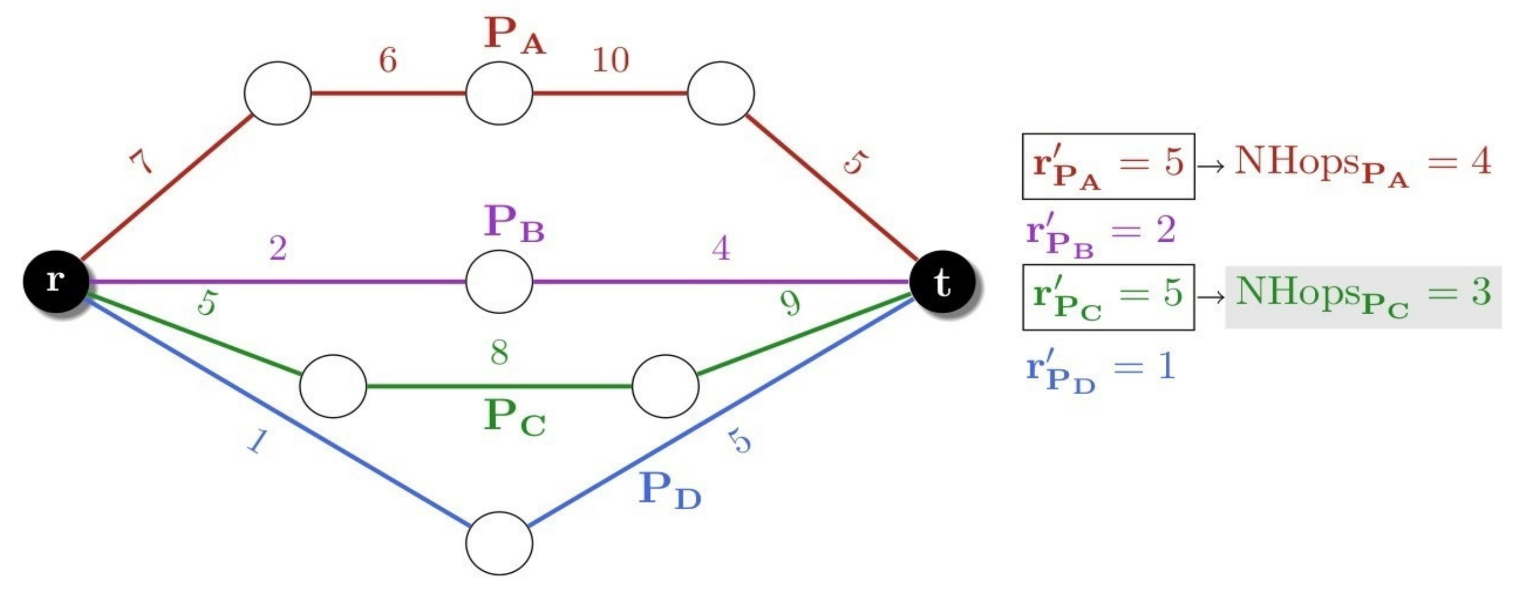
• Strategy 4. (Shortest-Widest, SW) [10]. This strategy searches for the path with the maximum Mean Residual Bandwidth from (Equation (8)). If there are several paths with the same maximum value, the strategy chooses the one with the minimum number of edges (hops). While the previous metrics are additive (the cost of the path is the sum of the costs of their links), the Residual Bandwidth is concave (the cost of the path is the cost of the link with minimum cost). Note that this metric is not properly a cost, but quite the opposite: it is a metric that measures the goodness of a link. Therefore, the goodness of a path will be associated with that of its worst link (the one with minimal residual bandwidth).
  Figure 3 helps understanding how this strategy works. The residual bandwidth appears on each link. According to the SW, paths $P_A$ and $P_C$ are firstly chosen (paths with the maximum residual bandwidth in their worst link), and between those two, path $P_C$ is selected, since it has the minimum number of hops.
• Strategy 5. (Fuzzy Shortest-Widest, FSW). It is the same than Strategy 4, but defining the Fuzzy Mean Residual Bandwidth measurement of each link $(i,j)$ as a triangular fuzzy number $(r_{ij}^{min},{\overline{r}}_{ij},r_{ij}^{max})$ where $r_{ij}^{min}$, ${\overline{r}}_{ij}$ and $r_{ij}^{max}$ are computed according to Equation (10),

  $$r_{ij}^{min}=c_{ij}-{\left[BW\right]}_{ij}^{max},{\overline{r}}_{ij}=c_{ij}-{\overline{\left[BW\right]}}_{ij},r_{ij}^{max}=c_{ij}-{\left[BW\right]}_{ij}^{min},$$

  (10)
  The path selection is performed following the fuzzy Dijkstra algorithm. This strategy is directly comparable with Strategy 4.
• Strategy 6: (Widest-Shortest, WS) [11]. This strategy consists of the inverse process of the SW. First, it searches for the path with the minimum number of hops. In case of several paths with the same number of hops, the strategy searches for the one with the maximum residual bandwidth.
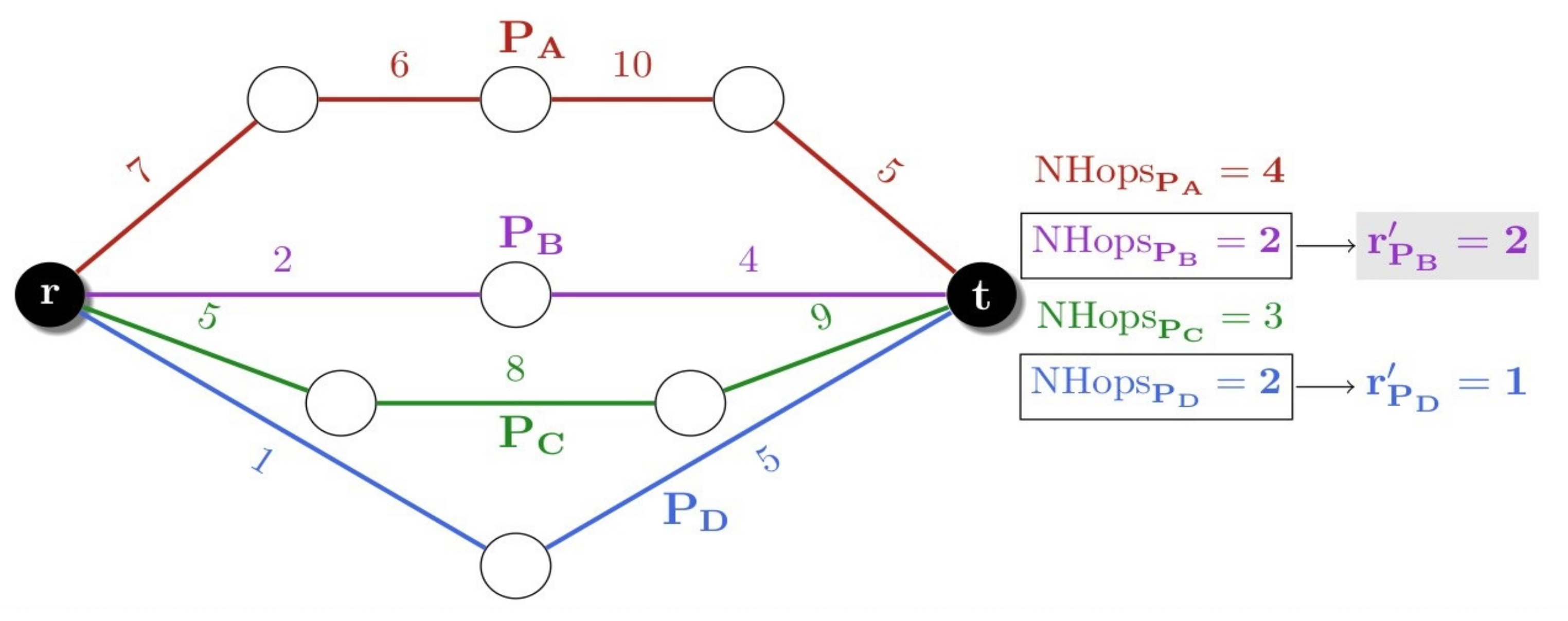
  Figure 4 shows the application of WS to the same network illustrated in Figure 3. The paths with the minimum number of hops are $P_B$ and $P_D$. Among them, the strategy WS chooses the path $P_B$ because it has the maximum Residual Bandwidth used bandwidth in its worst link.
• Strategy 7: (Fuzzy Widest-Shortest, FWS). Using the same definition of fuzzy cost as in Strategy 5, the same selection pattern is followed as in Strategy 6. This strategy competes with Strategy 6.

Finally, we propose a new strategy (Strategy 8), which uses a new fuzzy cost function that has no crisp equivalent since it is an empirical adaptation of the generalized fuzzy number model described above. This new strategy and its cost function are explained in detail below.

• Strategy 8. It can be verified that the smaller the bandwidth used during the interval $(n-1)$-th time (period where the measurements were made), the higher the degree of uncertainty in the values considered for the used bandwidth at the n-th time interval. We can explain the above statement by the following two factors,
  • The percentage of variation. When a link has a very low used bandwidth, a new connection causes a high relative variation in the value of the occupied bandwidth. On the contrary, if the used bandwidth is large, a new connection will have little impact on the relative variation.
  • The routing algorithm itself. The routing algorithm prioritizes the least used links so that the smaller the occupation of a link is, the most likely this parameter varies significantly in the next time interval.
  These reasons lead us to redefine the fuzzy number that describes the occupation in Strategy 3 (Equation (9)), which is multiplied by a coefficient. The Modified Fuzzy Normalized Used Bandwidth in a link $(i,j)$ is defined in Equation (11).

  $${\widetilde{Cost}}_{St8}=A\ast B^{-{\overline{\left[bw\right]}}_{ij}}{\widetilde{\left[bw\right]}}_{ij},$$

  (11)
  In practice, this operation produces a displacement to the right and a widening of the fuzzy number. In our experiments we set $A=10$ and $B=20$.

6. Experimentation and Results

6.1. Description of the Experiment

In this work, the simulator OMNET ++ [31] is used for the experimentation. The code used for the experiment and the configuration files can be downloaded from [32]. A flow-oriented simulation is performed to reduce the execution time of each simulation (the alternative packet-oriented simulation would require an execution time in the order of thousand times greater).

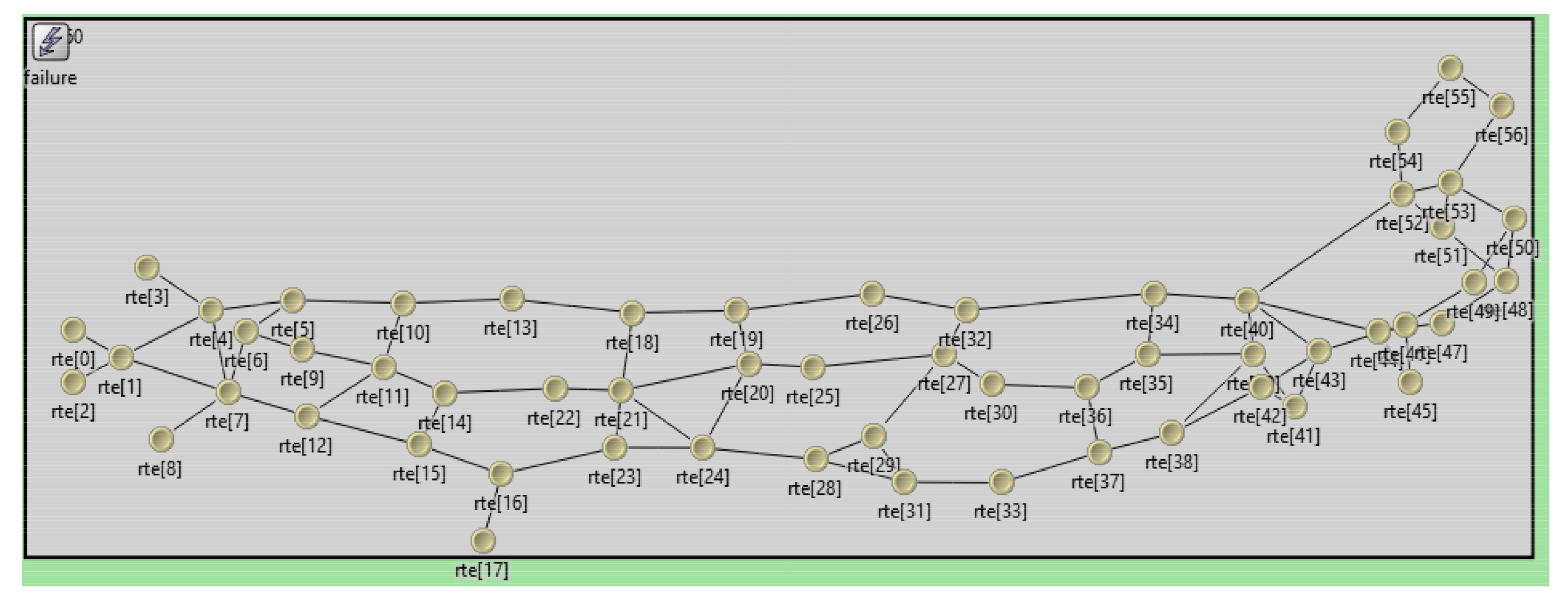
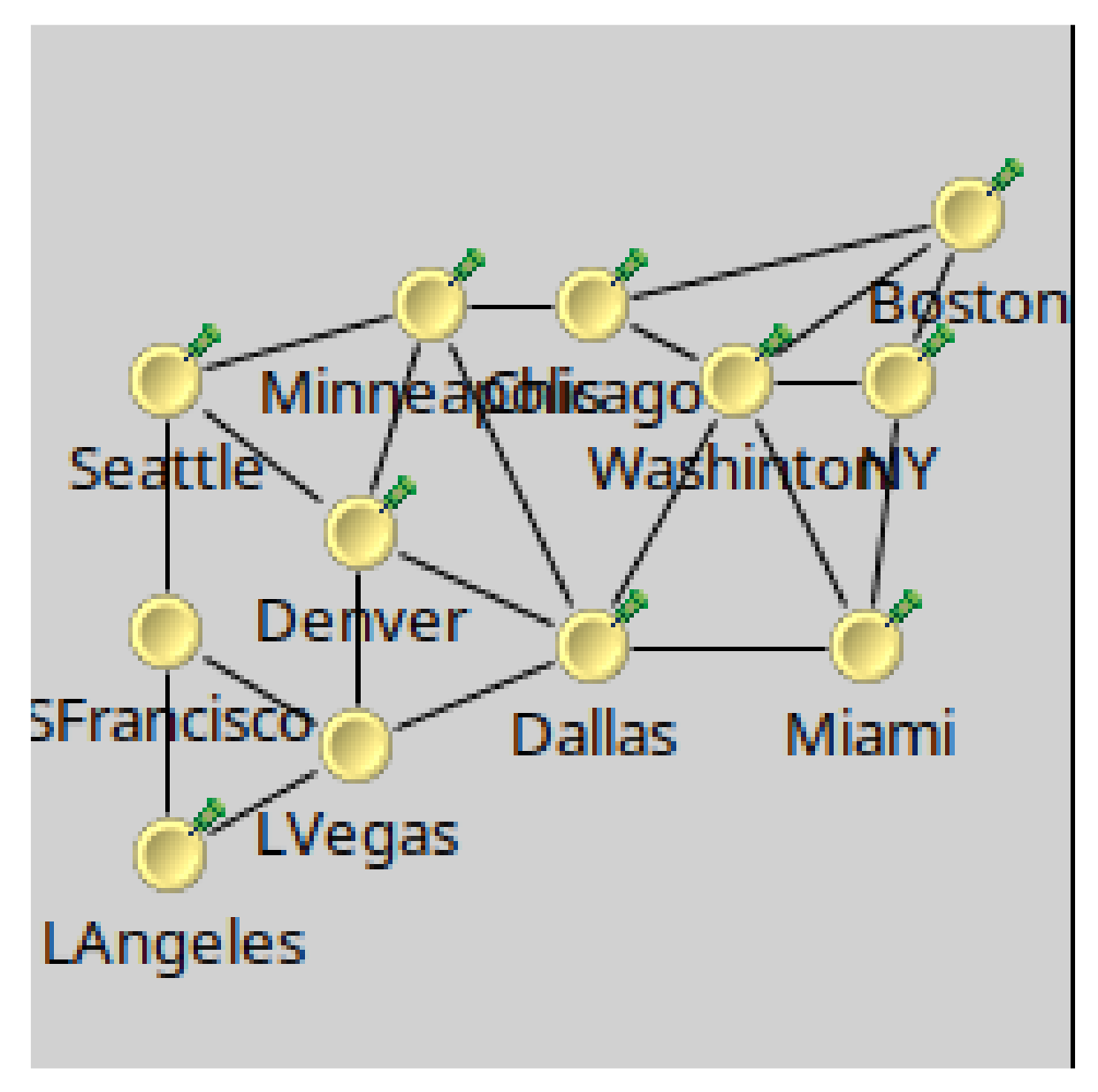
In our study, a 57-node and a 12-node networks were used. The first one is based on the topology of the backbone network of the Nippon Telegraph and Telephone (NTT). This topology has been extensively used in the related literature such as in [33]. The particular characteristics of our implementation can be found in the examples of the use of the OMNeT ++ simulator [31] (Figure 5). The second one is based on the topology of the National Science Foundation’s Network (NFSNET) (Figure 6) [34]. This network is obsolete today, but it has been used extensively in the study of routing protocols.

Our data loss model simulates an optical burst switching network (OBS) without storage. If a burst does not have enough bandwidth on a link, the information is discarded (that is, the information is lost) until there are enough resources. When there are not enough resources at any time during the burst lifetime, the complete burst is discarded. The model and source code required to carry out these simulations are found in [32].

To facilitate the reproduction of the experiments, we have carried out ten simulations with different seeds for each of the different strategies, where every node generates traffic with the same probability. We have adjusted the traffic in both networks to work in a close saturation mode, because we want to study the performance of the different strategies under these conditions. With low saturation, all the strategies can deliver the traffic successfully, and in high saturation conditions, the percentage of losses impacts on the network performance.

Table 1. Characteristics of the traffic used in the experiments with NTT network.

Description of the Parameters	Value
Call rate	Poisson Distribution with mean value 0.5 Calls/s
Call duration	Exponential Distribution with mean value $\mu =120$ s
Type of traffic	ON/OFF
Used Bandwidth over an ON period	30 Mbit/s
ON period	Exponential Distribution with mean value $\mu =5$ s
OFF period	Exponential Distribution with mean value $\mu =1$ s
Connection type	Symmetrical and bidirectional
Simulation time	10,000 s
Interval of time to update routing tables	300 s
Number of replications with different seeds	10

and

Table 2. Characteristics of the traffic used in the experiments with NFSNET network.

Description of the Parameters	Value
Call rate	Poisson Distribution with mean value 0.14 calls/s
Call duration	Exponential Distribution with mean value $\mu =60$ s
Type of traffic	ON/OFF
Used Bandwidth over an ON period	30 Mbit/s
ON period	Exponential Distribution with mean value $\mu =1$ s
OFF period	Exponential Distribution with mean value $\mu =1$ s
Connection type	Symmetrical and bidirectional
Simulation time	10,000 s
Interval of time to update routing tables	300 s
Number of replications with different seeds	10

indicate the features of the traffic used for the first and second network topologies, respectively.

Each parameter characterizing the traffic is described next:

• Call rate: Mean number of connections requests.
• Call duration: Interval of time at which the connection is active once it is established.
• Type of traffic: Data are transmitted for a specific time (burst with constant bandwidth) and they are not transmitted for another time interval.
• Used Bandwidth over an ON period: Resources required for a connection over an ON period. Since we are considering an ON period of 5 s and an OFF period of 1 s, the Mean Used Bandwidth for a connection is 25 Mb/s, that is, approximately, the Used Bandwidth of an Advanced Video Coding High Definition (AVCHD) connection. We use this value in order to work in conditions of saturation.
• ON period: Transmission period. It is modeled by a random distribution. In our case we use an exponential distribution with a mean of 5 s.
• OFF period: Period without transmission, that is, without consumption of resources. We use the same exponential function with a mean of 1 s. We force an off period to guarantee the competition of the burst.
• Connection type: Given a connection, both nodes can be source and destination simultaneously with the same consumption of resources. Thus, the connection is symmetrical and bidirectional.
• Simulation time: It is the simulated time assigned to each experiment (do not confuse with the duration of the simulation).
• Interval of time to update routing tables: Interval of time used to measure the average occupation of links and update the routing tables. Higher values in this parameter imply higher uncertainty in the measurements.

In our simulation scenario, source and destination nodes are randomly selected (with equal probability) among all the nodes in the network. Thus, there are multiple active source-destination pairs simultaneously.

In the networks, our magnitudes of interest are the total number of sent and received bytes by each node at each simulation interval.

From the previous values, we calculate the following metrics:

• Mean Delivery Rate (MDR): Total number of received bits divided by the total number of sent bits during an experiment. This value indicates the probability that a sent data is finally received. We use this value to obtain the GMDR.
• Global Mean Delivery Rate (GMDR): Mean of the MDR in ten experiments.
• Confidence interval (Computed with a probability of 0.95).

6.2. Results and Discussion

As a previous question, we raise some considerations about the suitability of applying the Dijkstra Algorithm in our problem. It is known that it can present two major drawbacks. On one hand, it does not converge in graphs with negative costs, which may imply a negative cycle. That could result in an infinite cycle, which will block the algorithm to find a solution [35]. On the other hand, when there is more than one shortest path between origin and destination nodes, Dijkstra algorithm will always provide the first one it finds, which can generate unbalanced solutions. The first drawback does not apply to our problem since all the links in our graphs have positive weights (the three parameters of our fuzzy numbers correspond to positive quantities measured in the network as described in Section 5.3). Regarding the second drawback, the probability that several paths generate the same value of their fuzzy costs is very low because of the high variability of their fuzzy triplets. Under these considerations, we can conclude that our fuzzy version of the Dijkstra algorithm is a reliable tool for solving our problem. In any case, we have alternatively implemented a Dijkstra algorithm for k-Shortest paths with k = 10, which extracts the 10 best routes. If there are several best routes with the same cost, it randomly selects one of them. Although in practice this algorithm is not necessary, its implementation is available in GitHub with the rest of the source codes of the simulator. When tested for our problems, we derived similar results.

To compare and rank the performance of the different strategies we calculate the Global Mean Delivery Rate (GMDR) such as it is defined above. This parameter informs about the ratio between the bits received and those sent during a complete simulation. Thus, comparison and ranking of the different strategies with different cost functions is possible.

Table 3. For each Strategy, the GMDR and confidence interval associated (NTT network).

Strategies	GMDR	Error	Conf. Interval $[{\mathit{C}\mathit{I}}_{min},{\mathit{C}\mathit{I}}_{max}]$
			${\mathbf{CI}}_{min}$	${\mathbf{CI}}_{max}$
Strategy 1	0.860	0.004	0.856	0.864
Strategy 2	0.861	0.0064	0.856	0.866
Strategy 3	0.870	0.004	0.866	0.874
Strategy 4	0.850	0.015	0.835	0.865
Strategy 5	0.857	0.013	0.843	0.870
Strategy 6	0.966	0.0025	0.963	0.968
Strategy 7	0.966	0.0026	0.9632	0.9684
Strategy 8	0.9982	0.0004	0.9978	0.9986

and

Table 4. For each Strategy, the GMDR and confidence interval associated. (NFSNET network).

Strategies	GMDR	Error	Conf. Interval $[{\mathit{C}\mathit{I}}_{min},{\mathit{C}\mathit{I}}_{max}]$
			${\mathbf{CI}}_{min}$	${\mathbf{CI}}_{max}$
Strategy 1	0.811	0.002	0.809	0.813
Strategy 2	0.809	0.0034	0.805	0.812
Strategy 3	0.832	0.003	0.83	0.835
Strategy 4	0.856	0.09	0.847	0.865
Strategy 5	0.862	0.065	0.856	0.869
Strategy 6	0.965	0.00045	0.964	0.9657
Strategy 7	0.965	0.00046	0.965	0.966
Strategy 8	0.9951	0.0001	0.9949	0.9952

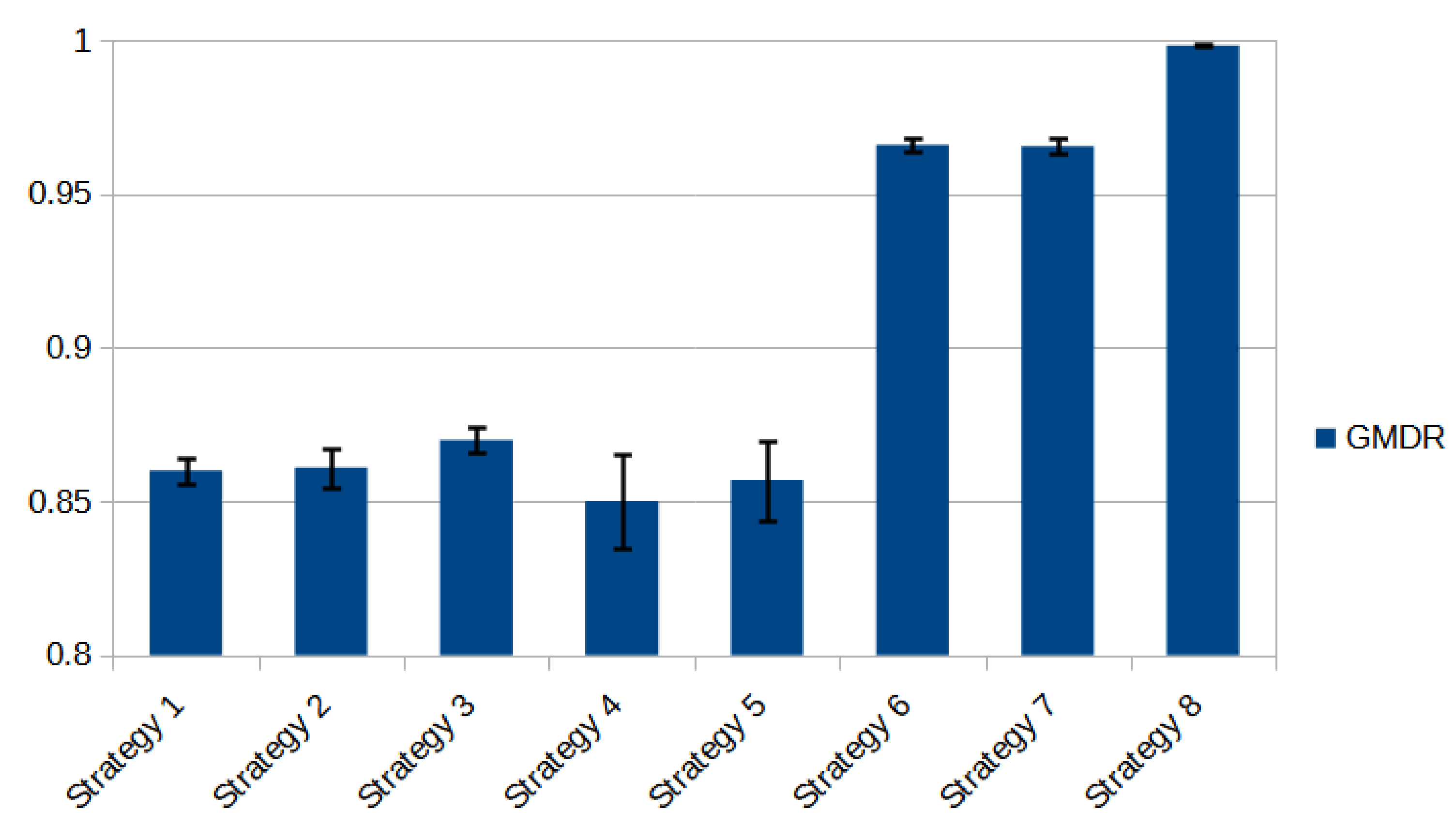
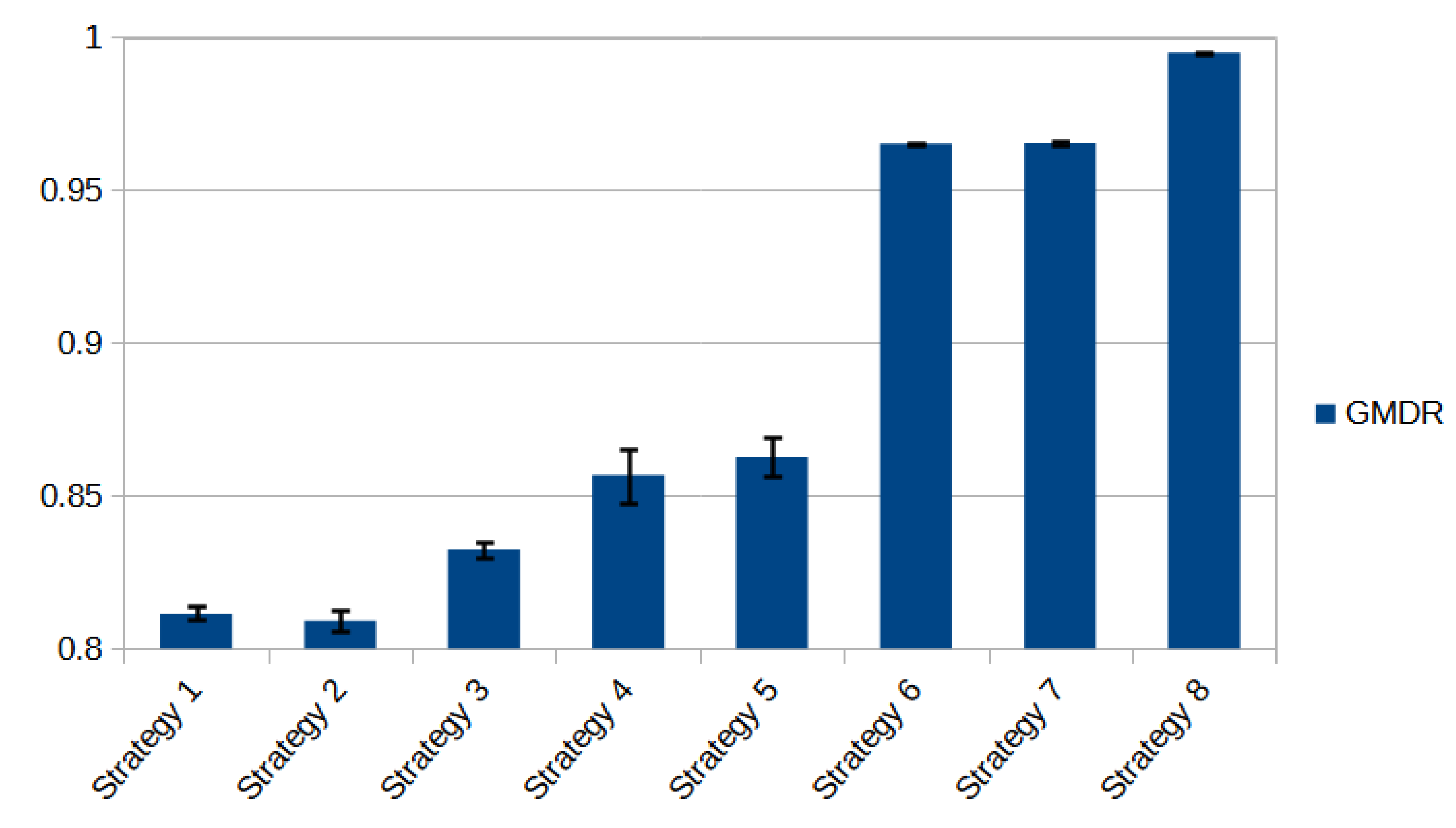
show these values together with the associated confidence intervals for NTT and NFSNET networks, respectively. Figure 7 and Figure 8 show the same information in a bar diagram for NTT and NFSNET. We can see that the behavior is qualitatively similar for both networks in all the analyzed strategies.

After a detailed analysis of each group of strategies, we obtain the following consideration for both studies:

When applying Strategy 3 (using Fuzzy Normalized Used Bandwidth as a cost function), we observe that the value of the GMDR surpasses its crisp equivalents (strategies 1 and 2), although in a small percentage. We find that confidence intervals are not overlapping. From the statistical point of view, this means that the results are distinguishable so that the resulting comparison has statistical validation.

Similarly, with Strategy 5 (Fuzzy Shortest-Widest), the value of the GMDR surpasses its crisp equivalent (Strategy 4), but their confidence intervals are overlapped. Thus, we must consider both results as equal from a statistical point of view.

Strategies 6 and 7 (Widest-Shortest and Fuzzy Widest-Shortest, respectively) have the same GMDR values with practically equal confidence intervals. We also observe that strategies 6 and 7 are superior to the previous ones (in the order of 10%). Our hypothesis in this regard is the advantage of these strategies working in a network close to saturation. Since these strategies search for paths with the minimum number of hops, they contribute to a lesser flow of information through the network. Therefore, Strategies 6 and 7 are benefited by the low consumption of resources when compared to Strategies 1 to 5.

Finally, as the main result of this study, we verify that Strategy 8 (proposed for the first time in this work), achieves a performance which is widely superior to all the previous ones. In particular, the value of GMDR is close to 1.

Therefore, the obtained results can be summarized with the following two statements:

• Fuzzy versions of the classical strategies are more efficient (or practically equal) than their corresponding crisp versions, although in a very narrow margin. Thus, we can say that our fuzzy modeling of a communications network correctly incorporates the uncertainty in the measurement variables, being competitive.
• Strategy 8, proposed by us, is the most efficient one with a clear advantage over the rest of the strategies. Specifically, it leads to a GMDR close to 1. This advantage comes from the definition of a new fuzzy cost function that incorporates our empirical knowledge about the effects of measurement uncertainty.

7. Conclusions

In this paper, we addressed the problem of searching the shortest path (or more efficient path, in a more general sense) between two nodes in a communication network, considering uncertainty in the measurements used in the cost function. The above referred uncertainty is inevitably caused by the network dynamics and the impossibility of making decisions with the instantaneous measurement of the state variables at each moment. Thus, in general, over a given time interval, decisions on the routing of information are made using measurements obtained in the previous time intervals, which, naturally, can differ from the current ones.

In order to incorporate our fuzzy cost functions and strategies into a communication network management system, we associate the network to a Type-V Fuzzy Graph. In this graph, nodes and links are clearly located (without uncertainty), but a triangular fuzzy number defines the cost for each connection. Moreover, a fuzzy version of Dijkstra’s routing algorithm was developed and exhaustively described. This is called Fuzzy Dijkstra Algorithm (FDA). Simulated experiments have shown its correct operation and competitiveness. It is essential to distinguish this approximation, in which the uncertainty lies on the value of the variables, from other approximations based on Fuzzy Inference, where these values are considered crisp (precise data) and the uncertainty lies on the decision rules used.

For our experimental study, we implemented the most commonly used cost functions and strategies in the management of real networks based on crisp values (e.g., these using the Instantaneous or Mean Used Bandwidth or Residual Bandwidth as cost function, Shortest-Widest (SW), Widest-Shortest (WS)) and we confronted them with their similar ones based on our definition of fuzzy costs. As an especially interesting contribution, we proposed a new fuzzy strategy (Strategy 8) that has no correspondence with any classic one, which adapts the definition of the fuzzy cost to the fact that the smaller the Used Bandwidth at the $(n-1)$-th time interval (where the measurements have been obtained) the more significant uncertainty in the Used Bandwidth value considered in the n-th time interval.

We made the experiments on two representative network topologies. Fuzzy Strategy 3 surpasses their analogous crisp ones (strategies 1,2) in a slightly, but statistically significant way. As for the fuzzy Strategies 5 and 7, we observed that they do not present statistically significant differences with their analogous crisp Strategies 4 and 6, respectively. However, our new fuzzy strategy (Strategy 8), with an effectiveness ratio very close to unity, clearly surpasses the rest of the analyzed strategies. Therefore, we conclude that our methodology to introduce the inherent uncertainty to the dynamic nature of the network in the routing algorithms has been successful.