On the Johnson–Tzitzeica Theorem, Graph Theory, and Yang–Baxter Equations

Abstract

This paper presents several types of Johnson–Tzitzeica theorems. Graph diagrams are used in this analysis. A symmetric scheme is derived, and new results are obtained and open problems stated. We also present results relating the graphs and the Yang–Baxter equation. This equation has certain symmetries, which are used in finding solutions for it. All these constructions are related to integrable systems.

1. Introduction

There are several purposes of the current work: to present the Johnson–Tzitzeica theorem and related (open) problems, to relate the Johnson–Tzitzeica theorem to graph theory, and to point out possible applications of the Johnson–Tzitzeica theorem in integrable systems and in the Yang–Baxter equation theory. Historical aspects are also considered.

According to [1], a set of Johnson circles refers to three circles of equal radius and a common point of intersection. In the Johnson–Tzitzeica theorem, “the figure is so simple (especially as it can be drawn and the theorem verified with a coin or other circular object) that it seems almost out of the question that the fact can have escaped detection. Even if geometers have overlooked it, someone must have noticed it in casually drawing circles. But if this were the case, it seems a theorem of sufficient interest to receive some prominence in the literature, and therefore ought to be well known” (cf. [2]).

In the next section, we present the Johnson–Tzitzeica theorem. A general symmetric scheme is derived, some open problems proposed, and a new theorem proven. There exists a whole field of discrete integrable geometry, where concepts from elementary geometry to nonlinear continuum or discrete systems of equations are studied. The most similar ideas can be found in a series of papers by A. Doliwa, where the elementary incidence geometry is a source of interesting (usually generic) problems in the theory of completely integrable systems. The paper [3] on circular lattices and then Desargues maps entered into the scene, leading to several steps to the Yang–Baxter equations through integrable systems and the famous Hirota–Miwa equations (see, for example, the papers [4,5,6]).

In Section 1, we associate a graph diagram with the Johnson–Tzitzeica theorem. This point of view eventually leads to new results both in geometry and in graph theory. Section 4 is a gentle introduction to the Yang–Baxter equation (see, for example, [7,8,9,10,11,12]). This equation has certain symmetries, which are used in finding solutions for it, and it plays an important role in integrable systems. V. Drinfeld (see [13]) suggested considering “set-theoretical” solutions to the Yang–Baxter equation (see also [14,15]). We first restrict our attention to the set-theoretical solutions. We recall that graph diagrams are important in the proof of a theorem and in visualizing some results. We present the Yang–Baxter equation in the vectorial space framework, proposing other similar equations. The relationship among these equations are studied using a graph diagram. Notice that the method presented in in the beginning of this section could be applied for finding solutions to them. The last section presents some historical aspects related to the Tzitzeica–Johnson theorem, several remarks (on integrable systems), and some research problems.

2. The Tzitzeica–Johnson Theorem and Pictorial Mathematics

In a talk at the 12th International Workshop on Differential Geometry and Its Applications, UPG Ploiesti 2015, Florin Caragiu explained that there exists a special mathematical discourse, called “proofs without words”. This discourse uses pictures or diagrams in order to boost the intuition of the reader (see [16,17]). The pictorial (diagrammatic) style of mathematical language is much appreciated by both educators and researchers in mathematics. Being very easy to grasp, some pictorial-style problems are similar to some nuts being small, but for which we need an entire “artillery” in order to crack them.

We now consider the Tzitzeica–Johnson problem (see, for example, [18]).

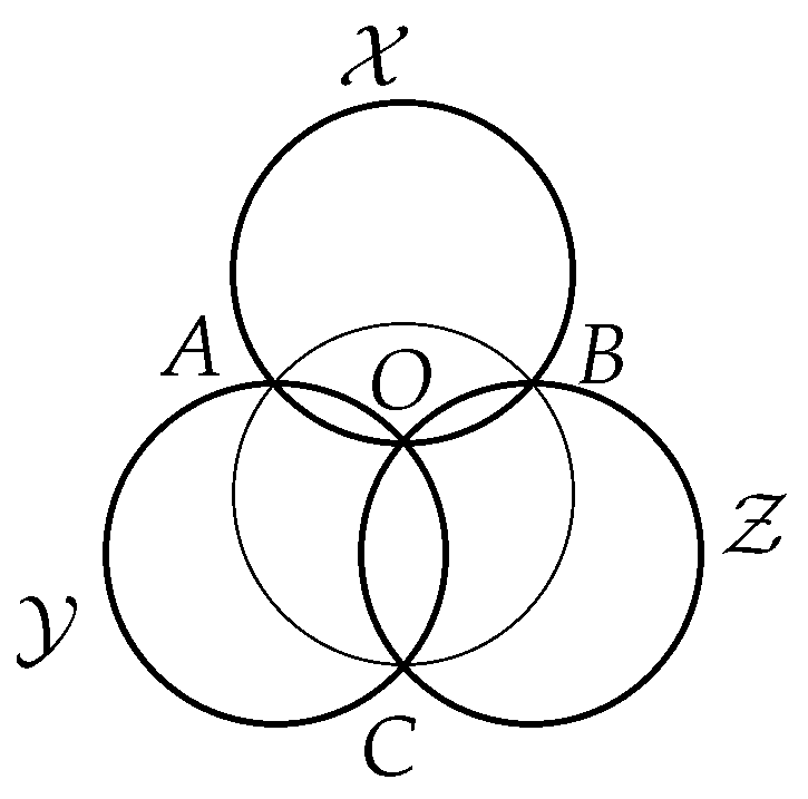
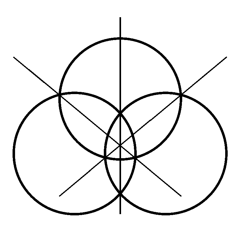
Let $\mathcal{X}$, $\mathcal{Y}$, and $\mathcal{Z}$ be three circles of radius r. Let us suppose that $\mathcal{X}\cap \mathcal{Y}=\{O,A\}$ $\mathcal{X}\cap \mathcal{Z}=\{O,B\}$, and $\mathcal{Y}\cap \mathcal{Z}=\{O,C\}$. Then, there exists a circle of radius $r$ through A, B, and C (see Figure 1).

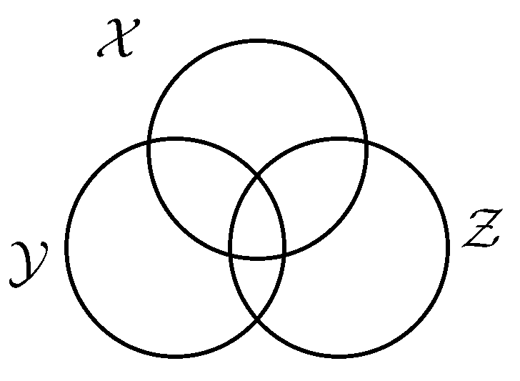
The above theorem can be included in a more general scheme (see Figure 2).

One could include in this scheme the inclusion–exclusion principle, for three sets:

$|X\cup Y\cup Z|=\left|X\right|+\left|Y\right|+\left|Z\right|-|X\cap Y|-|X\cap Z|-|Y\cap Z|+|X\cap Y\cap Z|$.

Let, for example, the case be as follows: $\left|X\right|=\left|Y\right|=\left|Z\right|=7$, $|X\cap Y|=|X\cap Z|=|Y\cap Z|=1$, and $|X\cap Y\cap Z|=1$. Then, there exists a set T, with $\left|T\right|=7$ that contains elements from all possible (sub)sets.

One could better visualize the relationship between the inclusion–exclusion principle and the mathematical scheme from Figure 2, if we represent the elements of the sets $X,Y,Z$, and T as circular lattice points.

Notice that Tzitzeica–Johnson’s theorem has many generalizations [18] and interpretations related to the above mathematical scheme (from Figure 2).

The dual Desargues theorem can be interpreted in the light of the above scheme by using arrangements of (three) colored lines.

The hypothesis is as follows:

$\mathcal{X}=\left\{\right(d,f,h)suchthatd\cap f\cap h=P\}$

$\mathcal{Y}=\{(d^{\prime },f,h^{\prime })suchthat{d}^{\prime }\cap f\cap h^{\prime }=Q\}$

$\mathcal{Z}=\{(d^{″},f,h^{″})suchthat{d}^{″}\cap f\cap h^{″}=R\}$

$\mathcal{X}\cap \mathcal{Y}\cap \mathcal{Z}=\left\{f\right\}$

$\mathcal{X}\cap \mathcal{Y}=\{A,A^{\prime }\}\cup \left\{f\right\}$

$\mathcal{Y}\cap \mathcal{Z}=\{B,B^{\prime }\}\cup \left\{f\right\}$

$\mathcal{X}\cap \mathcal{Z}=\{C,C^{\prime }\}\cup \left\{f\right\}$

The conclusion is as follows:

There exists a triple $(l,m,n)$ through $A,A^{\prime },B,B^{\prime },C$, and $C^{\prime }$.

Tzitzeica–Johnson’s theorem can be interpreted in terms of disks:

– “If three disks of the same radius have a common point of intersection, then they contain inside of their union a forth disk with the same radius.”;

– “If three disks $\mathcal{X}$, $\mathcal{Y}$ and $\mathcal{Z}$ of the same radius have a common point, then there exists a forth disk of the same radius which includes $(\mathcal{X}\cap \mathcal{Y})\cup (\mathcal{X}\cap \mathcal{Z})\cup (\mathcal{Y}\cap \mathcal{Z})$.”

It is an open problem to prove a similar statement for a domain bounded by an arbitrary closed convex curve. In other words, we conjecture that if we consider a domain $\mathcal{X}$ bounded by an arbitrary closed convex curve and two copies of $\mathcal{X}$, denoted by $\mathcal{Y}$ and $\mathcal{Z}$, such that $\mathcal{X}\cap \mathcal{Y}\cap \mathcal{Z}\ne \varnothing$, then there exists another copy of $\mathcal{X}$, denoted by $\mathcal{T}$, such that $(\mathcal{X}\cap \mathcal{Y})\cup (\mathcal{X}\cap \mathcal{Z})\cup (\mathcal{Y}\cap \mathcal{Z})\subset \mathcal{T}\subset \mathcal{X}\cup \mathcal{Y}\cup \mathcal{Z}$.

Even the case when $\mathcal{X}$ is a square is very difficult.

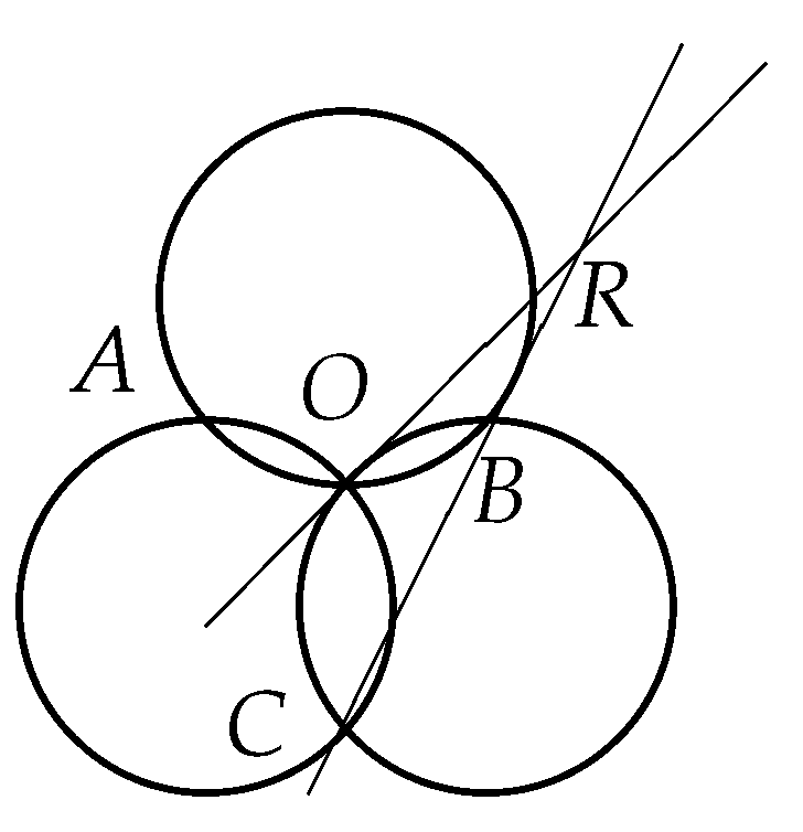
We now propose a new construction for a set of Johnson circles (in Figure 3).

At this moment, we can present a new theorem.

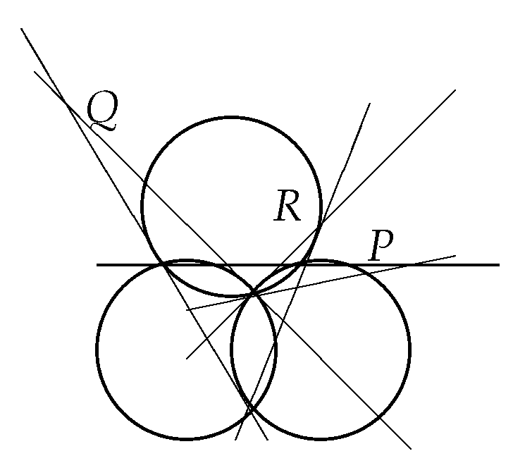
For a set of Johnson circles, let R be the intersection point between the tangent in O to the third circle and the line $BC$, Q the intersection point between the tangent in O to the second circle and the line $AC$, and P the intersection point between the tangent in O to the first circle and the line $AB$.

Then, P, Q, and R are collinear points (see Figure 4 below).

Proof. 

The proof of the above theorem is based on the properties of the power of a circle and on Desargues’ theorem. It is the limit case from Figure 5. □

It is an open problem to find the relationship between the line through P, Q, and R and the circle through A, B, and C.

3. The Tzitzeica–Johnson Theorem and Graph Diagrams

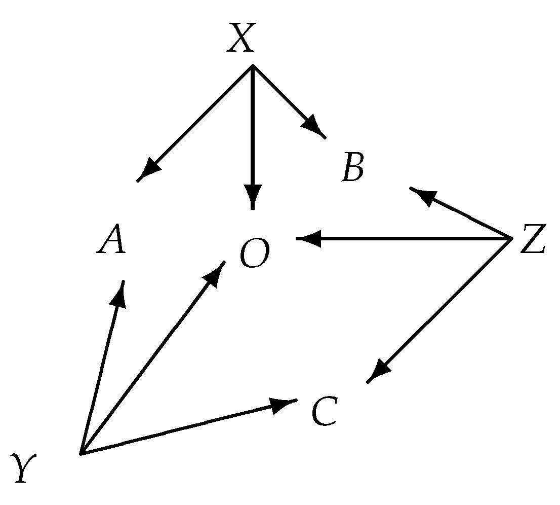
We would like to transfer the Tzitzeica–Johnson theorem into the graph theory setting. We first associate a graph diagram with the Johnson–Tzitzeica theorem (recall Figure 1). If, we denote by X the center of the circle $\mathcal{X}$, by Y the center of the circle $\mathcal{Y}$, and by Z the center of the circle $\mathcal{Z}$, then we could consider the following graph diagram related to the Johnson–Tzitzeica theorem (see Figure 6).

The conclusion of this Johnson–Tzitzeica theorem for graph diagrams is that this graph, from Figure 6, could be embedded in a regular graph. In other words, we would like the in-degree or the out-degree of each vertex of the new graph to be equal to three.

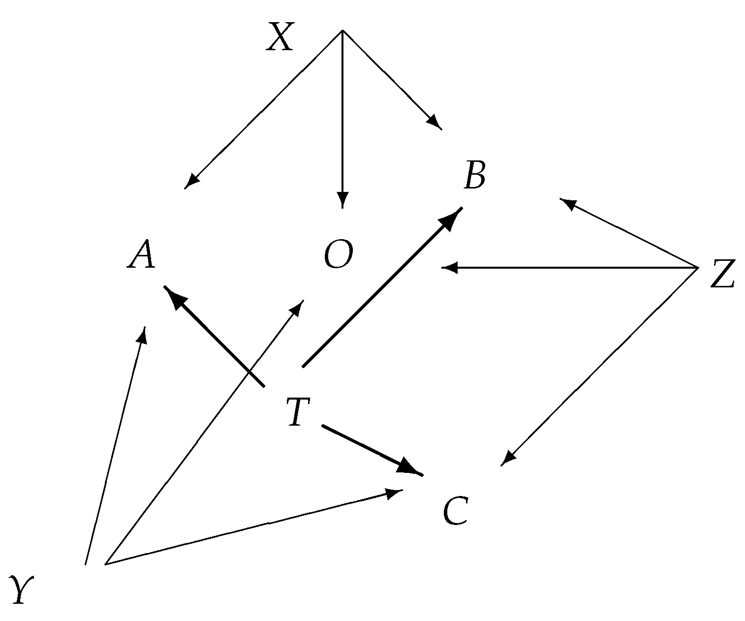
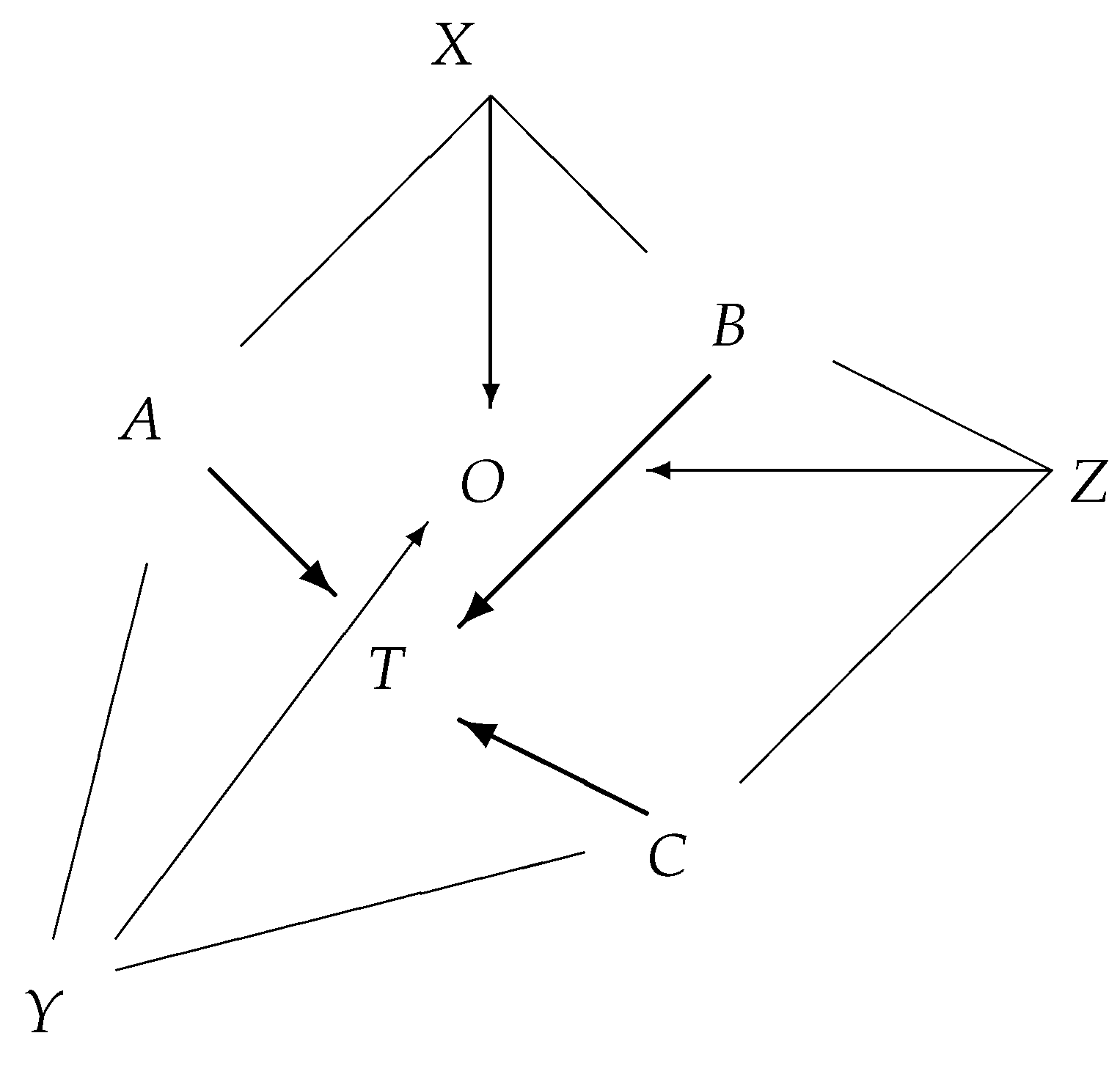
The proof is given in Figure 7.

We consider an example of how this approach could lead to a geometry theorem.

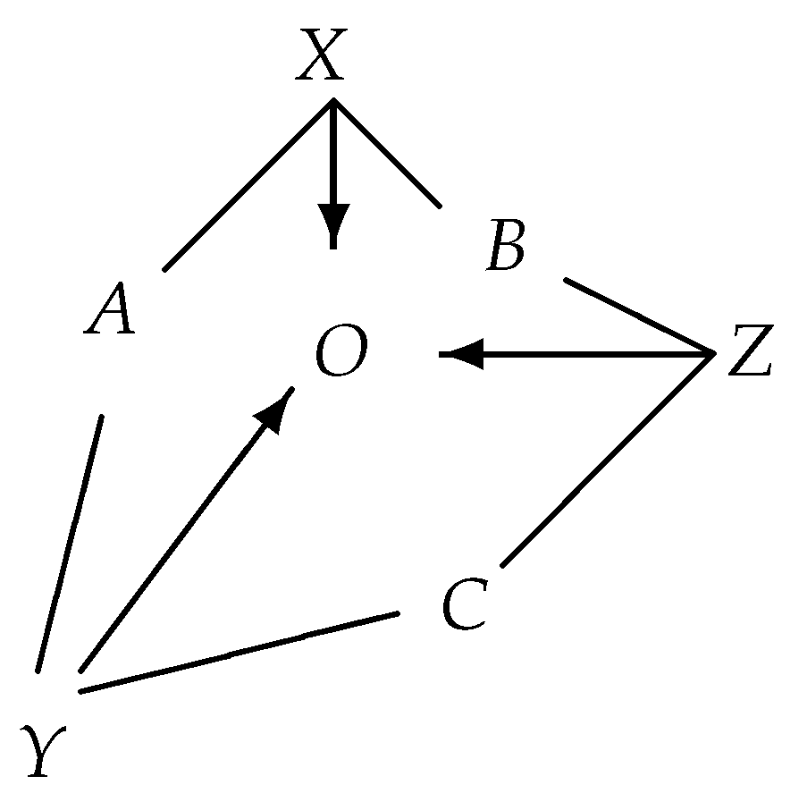
We now consider a mixed graph related to a set of Johnson circles (see Figure 8).

We embed this mixed graph into a (regular) mixed graph (see Figure 9).

Going back to geometry, we obtain a new theorem.

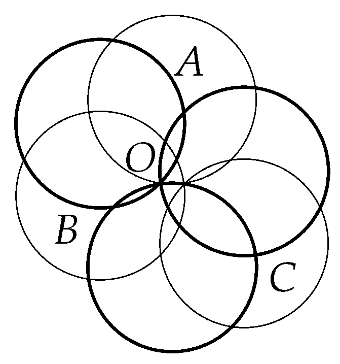
For a set of Johnson circles, the circles of radius r with centers A, B, and C meet at one point (see Figure 10).

Proof. 

According to the Tzitzeica–Johnson theorem, there exists a circle of radius r through A, B, and C. Let T be the center of this circle. It follows easily that the circles of radius r with centers A, B, and C meet at the point T (see Figure 10). □

The question of how to embed an oriented graph in a regular graph (how many vertices need to be added, etc.) could be a research theme in graph theory (with implications for geometry).

4. Yang–Baxter Equations, Relations, and Graphs

If X is a set, let $S:X\times X\to X\times X$ be a function, $S^{12}=S\times I$ and $S^{23}=I\times S$.

Using the above notation, the set-theoretical Yang–Baxter equation reads:

$$S^{12}\circ S^{23}\circ S^{12}=S^{23}\circ S^{12}\circ S^{23}$$

(1)

We use the following notation for a relation R on the set X: we denote by $R^{op}$ the opposite relation of R; we denote by $\overline{R}$ the complementary relation of R.

(D. Hobby and F. F. Nichita [19]) Let X be a set and $R\subset X\times X$ a reflexive relation on X. We define the function $S=S_R:X\times X\to X\times X$ by $S(u,v)=\left\{\begin{array}{cc}(u,v),\hfill & \mathrm{if}(u,v)\in R;\hfill \\ (v,u),\hfill & \mathrm{otherwise}.\hfill \end{array}\right.$

Then, S satisfies (1) if and only if $R\cup R^{op}$ is an equivalence relation and $\overline{R}$ is a strict partial order relation on each class of $R\cup R^{op}$.

The proof from [19] relies heavily on graph diagrams. After many cases are investigated, the theorem is proven. An example using Hasse diagrams and graphs is then presented.

For each of the relations represented by the graphs from Figure 6 and Figure 7, if we consider $S_{\overline{R}}$ (S for the complementary relation), we obtain a solution for (1).

We continue the section working over a generic field k. The tensor products are defined over k. Let V be a vector space over k. Let $I=I_V:V\to V$ be the identity map of the space V. We denote by $\tau :V\otimes V\to V{\otimes }_{B}V$ the twist map defined by $\tau \left(v{\otimes }_{B}w\right)=w{\otimes }_{B}v$. For $R:V{\otimes }_{B}V\to V{\otimes }_{B}V$, a k-linear map, let $R^{12}=R{\otimes }_{B}I,R^{23}=I{\otimes }_{B}R:V{\otimes }_{B}V{\otimes }_{B}V\to V{\otimes }_{B}V{\otimes }_{B}V.$ In a similar manner, we denote by $R^{13}$ a linear map acting on the first and third component of $V\otimes V\otimes V$. It turns out that $R^{13}=\left(I{\otimes }_B\tau \right)\left(R{\otimes }_{B}I\right)\left(I{\otimes }_B\tau \right)$.

A Yang–Baxter operator is a k-linear map $R:V{\otimes }_{B}V\to V{\otimes }_{B}V$, which satisfies the braid condition (the Yang–Baxter equation):

$$R^{12}\circ R^{23}\circ R^{12}=R^{23}\circ R^{12}\circ R^{23}.$$

(2)

Usually, we also require that the map R be invertible.

An important observation is that if R satisfies (2), then both $R\circ \tau$ and $\tau \circ R$ satisfy the quantum Yang–Baxter equation (QYBE):

$$R^{12}\circ R^{13}\circ R^{23}=R^{23}\circ R^{13}\circ R^{12}.$$

(3)

We now consider other (systems of) equations for a k-linear map $R:V{\otimes }_{B}V\to V{\otimes }_{B}V$:

$$R^{12}\circ R^{23}=R^{13}\circ R^{12}=R^{23}\circ R^{13}$$

(4)

$$R^{23}\circ R^{12}=R^{12}\circ R^{13}$$

(5)

$$R^{12}\circ R^{13}\circ R^{12}\circ R^{23}=R^{23}\circ R^{13}\circ R^{23}\circ R^{12}$$

(6)

$$(R^{12}\circ R^{23}\circ R^{12}-R^{23}\circ R^{12}\circ R^{23})\circ (R^{12}\circ R^{13}\circ R^{23}-R^{23}\circ R^{13}\circ R^{12})=0$$

(7)

$$R=XY,R^{12}\circ X^{13}\circ R^{23}\circ Y^{12}=R^{23}\circ X^{13}\circ R^{12}\circ Y^{23}$$

(8)

$$R\circ R=I\otimes I$$

(9)

$$R^{12}{R}^{23}{R}^{13}{R}^{23}+R^{23}{R}^{12}{R}^{13}{R}^{12}=R^{23}{R}^{12}{R}^{23}{R}^{12}{R}^{13}{R}^{23}+R^{12}{R}^{23}{R}^{12}{R}^{23}{R}^{13}{R}^{12}$$

(10)

(i) If a k-map $R:V{\otimes }_{B}V\to V{\otimes }_{B}V$ verifies (4) and (5), then R is a common solution for (2) and (3);

(ii) If a k-map $R:V{\otimes }_{B}V\to V{\otimes }_{B}V$ verifies (2) or (3), then R is a solution for (7);

(iii) If a k-map $R:V{\otimes }_{B}V\to V{\otimes }_{B}V$ verifies (2) or (3), then it is a solution for (8);

(iv) If a k-map $R:V{\otimes }_{B}V\to V{\otimes }_{B}V$ verifies (2), (3) and (9), then it is a solution for (6);

(v) If a k-map $R:V{\otimes }_{B}V\to V{\otimes }_{B}V$ verifies (7) and (9), then it is a solution for (10).

Proof. 

(i) We only sketch the proof of the first claim: $R^{23}\circ R^{12}\circ R^{23}=R^{23}\circ R^{13}\circ R^{12}=R^{12}\circ R^{23}\circ R^{12}$, etc (see [12]).

(ii) The proof is direct;

(iii) For $X=R$ and $Y=I{\otimes }_{B}I$, this equation becomes Equation (3). For $X=I{\otimes }_{B}I$ and $Y=R$, this equation becomes Equation (3);

(iv) $R^{23}\circ R^{13}\circ R^{23}\circ R^{12}=R^{23}\circ R^{13}\circ R^{12}\circ R^{12}\circ R^{23}\circ R^{12}=R^{12}\circ R^{13}\circ R^{23}\circ R^{23}\circ R^{12}\circ R^{23}=R^{12}\circ R^{13}\circ R^{12}\circ R^{23}$;

(v) The proof is direct. □

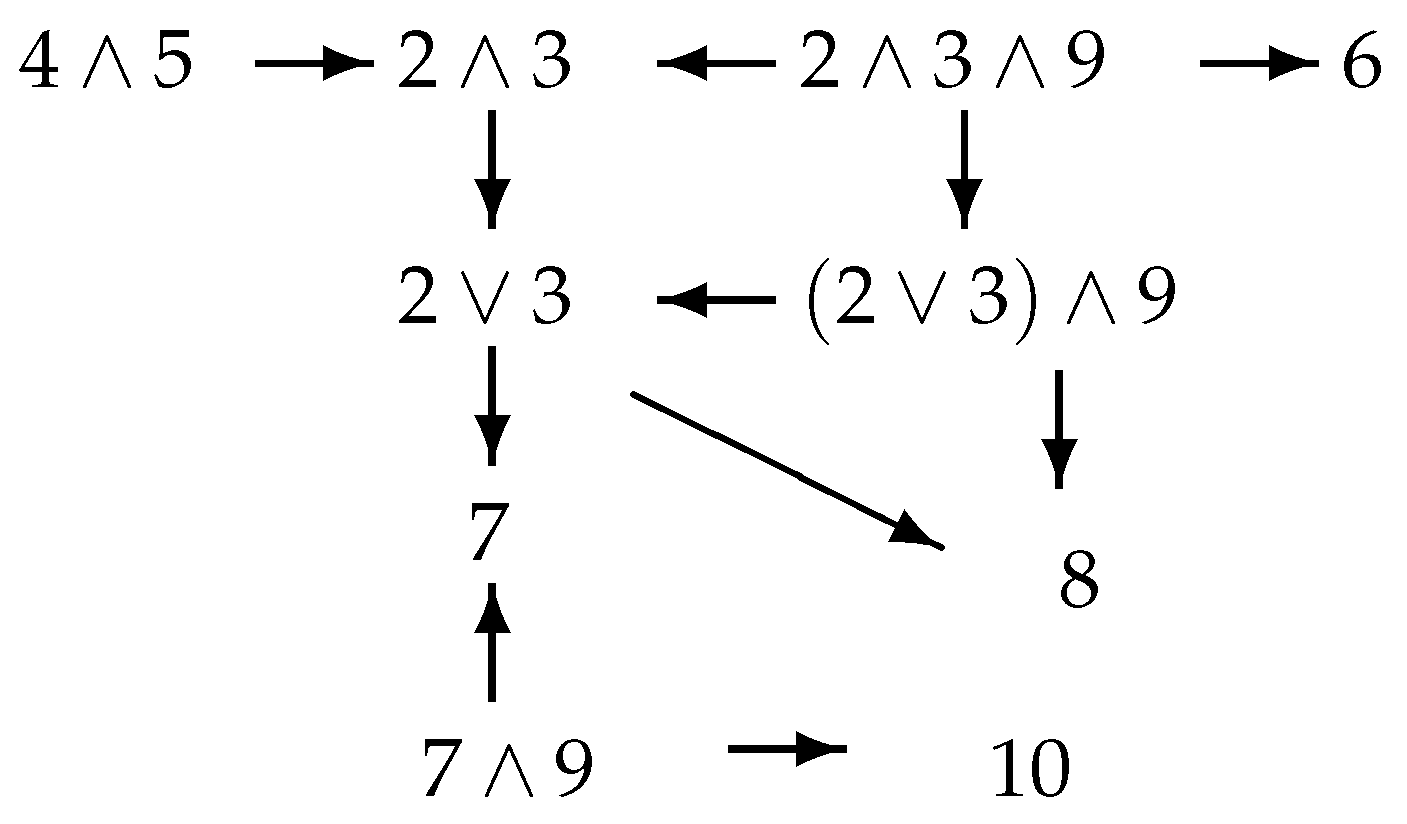
We could present the above results using a graph diagram (see Figure 11).

5. Applications, Historical Aspects, and Final Comments

The Romanian mathematician Gheorghe Tzitzeica is also known for a result on the geometry of circles and triangles in the plane, referred to as Tzitzeica’s five lei coin problem, a problem he proposed (and solved) at the “Gazeta Matematica” contest in Galati in 1908. The problem was posed independently by Roger Arthur Johnson in 1916 [20,21].

There exists a whole field of discrete integrable geometry, where similar concepts, from elementary geometry to nonlinear continuum or discrete systems of equations, have been studied for many years. The paper [3] on circular lattices where the Miguel theorem plays the crucial role and then Desargues maps entered into the scene, leading to several steps to the Yang–Baxter equations. It can be shown that the Miguel theorem implies the dual of the Johnson–Tzitzeica theorem (in this case we take into consideration the midpoints of the edges of the given triangle).

Related to another section of the current paper, one could attempt to find solutions for Equations (4)–(10) using the function $S_R$ (see Theorem Section 4).

References

- Circles, J. From Wikipedia, the Free Encyclopedia. Available online: https://en.wikipedia.org/wiki/Johnson_circles (accessed on 28 October 2021).
- Johnson, R.A. A Circle Theorem. Am. Math. Mon. 1916, 23, 161–162. [Google Scholar] [CrossRef]
- Cieslinski, J.; Doliwa, A.; Santini, P.M. The integrable discrete analogues of orthogonal coordinate systems are multidimensional circular lattices. Phys. Lett. A 1997, 235, 480–488. [Google Scholar] [CrossRef]
- Doliwa, A. Desargues maps and the Hirota–Miwa equation. Proc. R. Soc. A 2010, 466, 1177–1200. [Google Scholar] [CrossRef] [Green Version]
- Doliwa, A. Non-Commutative Rational Yang–Baxter. Lett. Math. Phys. 2014, 104, 299–309. [Google Scholar] [CrossRef] [Green Version]
- Doliwa, A.; Sergeev, S.M. The pentagon relation and incidence geometry. J. Math. Phys. 2014, 55, 063504. [Google Scholar] [CrossRef] [Green Version]
- Yang, C.N. Some exact results for the many-body problem in one dimension with repulsive delta-function interaction. Phys. Rev. Lett. 1967, 19, 1312–1315. [Google Scholar] [CrossRef]
- Baxter, R.J. Exactly Solved Models in Statistical Mechanics; Academic Press: London, UK, 1982. [Google Scholar]
- Baxter, R.J. Partition function for the eight-vertex lattice model. Ann. Phys. 1972, 70, 193–228. [Google Scholar] [CrossRef]
- Nichita, F.F. Mathematics and Poetry · Unification, Unity, Union. Union. Sci. 2020, 2, 72. [Google Scholar]
- Nichita, F.F. Unification Theories: Examples and Applications. Axioms 2018, 7, 85. [Google Scholar] [CrossRef] [Green Version]
- Badea, I.R.; Mocanu, C.E.; Nichita, F.F.; Păsărescu, O. Applications of Non-Standard Analysis in Topoi to Mathematical Neurosciences and Artificial Intelligence: Infons, Energons, Receptons (I). Mathematics 2021, 9, 2048. [Google Scholar] [CrossRef]
- Drinfeld, V.G. Quantum groups. In Proceedings of the International Congress of Mathematicians, Berkeley, CA, USA, 3–11 August 1986; American Mathematical Society: Berkeley, CA, USA, 1986. [Google Scholar]
- “Noncommutative and Non-Associative Structures, Braces and Applications”, Malta, 11–15 March 2018. Available online: https://sites.google.com/site/alcodaworkshop/ (accessed on 28 October 2021).
- Smoktunowicz, A.; Alicja Smoktunowicz, A. Set-theoretic solutions of the Yang–Baxter equation and new classes of R-matrices. Linear Algebra Its Appl. 2018, 546, 86–114. [Google Scholar] [CrossRef] [Green Version]
- Nichita, F.F. On Jordan Algebras and Unification Theories; Revue Roumaine de Mathematiques Pures et Appliquees, Romanian Academy: Bucharest, Romania, 2016; Volume 61, pp. 305–316. [Google Scholar]
- Caragiu, F.; Lemeni, A.; Trausan-Matu, S. Language in Mathematics, Science and Artificial Intelligence vs. Language in Theology; Dialog in Absolut/ieromonah Ghelasie Gheorghe: Bucharest, Romania, 2007; pp. 293–3007. [Google Scholar]
- Moise, L.D.; Cristea, R. Gheorghe Titeica – contemporary geometry / reverbertii si permanente ale geometriei in contemporaneitate. In Proceedings of the Conferinta Nationala de Invatamant Virtual, Editia a XI-a, Bucharest, Romania, 25–26 October 2013; pp. 150–156. [Google Scholar]
- Hobby, D.; Nichita, F.F. Solutions for the set-theoretical Yang–Baxter equation derived from relations. Acta Univ. Apulensis 2012, 30, 15–23. [Google Scholar]
- Tzitzeica, G. From Wikipedia, the Free Encyclopedia. Available online: https://en.wikipedia.org/wiki/Gheorghe_%C8%9Ai%C8%9Beica (accessed on 26 October 2021).
- Tzitzeica, G. Geometry Problems…and beyond Them; SIGMA: Bucharest, Romania, 2014. (In Romanian) [Google Scholar]
Figure 1.
The three coins problem (Tzitzeica 1908; Johnson 1916).
Figure 2.
A mathematical scheme. If , , and have certain properties, then there exists a related , with the same properties.
Figure 3.
The tangent to the third circle in O meets the line in R.
Figure 4.
The points P, Q, and R are collinear.
Figure 5.
The limit case of the following picture implies our theorem.
Figure 6.
The hypothesis of a Johnson–Tzitzeica theorem for graph diagrams: we consider an oriented graph with 7 vertices and 9 oriented edges.
Figure 7.
Proof of a Johnson–Tzitzeica theorem for graph diagrams: there exist a new vertex T and 3 oriented arrows making all the vertices in the graph sinks or sources of degree 3.
Figure 8.
A mixed graph.
Figure 9.
A mixed graph leading to a geometry theorem.
Figure 10.
The circles of radius r with centers A, B, and C meet at the point T.
Figure 11.
A graph diagram describing the relations among the above equations.
Publisher’s Note: MDPI stays neutral with regard to jurisdictional claims in published maps and institutional affiliations. |
© 2021 by the author. Licensee MDPI, Basel, Switzerland. This article is an open access article distributed under the terms and conditions of the Creative Commons Attribution (CC BY) license (https://creativecommons.org/licenses/by/4.0/).
Share and Cite
MDPI and ACS Style
Nichita, F.F. On the Johnson–Tzitzeica Theorem, Graph Theory, and Yang–Baxter Equations. Symmetry 2021, 13, 2070. https://doi.org/10.3390/sym13112070
AMA Style
Nichita FF. On the Johnson–Tzitzeica Theorem, Graph Theory, and Yang–Baxter Equations. Symmetry. 2021; 13(11):2070. https://doi.org/10.3390/sym13112070
Chicago/Turabian StyleNichita, Florin F. 2021. "On the Johnson–Tzitzeica Theorem, Graph Theory, and Yang–Baxter Equations" Symmetry 13, no. 11: 2070. https://doi.org/10.3390/sym13112070
Note that from the first issue of 2016, this journal uses article numbers instead of page numbers. See further details here.