Article

Data Anomaly Detection of Bridge Structures Using Convolutional Neural Network Based on Structural Vibration Signals

School of Architecture and Civil Engineering, Xiamen University, Xiamen 361005, China
*
Author to whom correspondence should be addressed.
Symmetry 2021, 13(7), 1186; https://doi.org/10.3390/sym13071186
Submission received: 5 June 2021 / Revised: 19 June 2021 / Accepted: 25 June 2021 / Published: 30 June 2021
(This article belongs to the Special Issue Symmetry in Structural Health Monitoring)

Abstract

:
Structural monitoring provides valuable information on the state of structural health, which is helpful for structural damage detection and structural state assessment. However, when the sensors are exposed to harsh environmental conditions, various anomalies caused by sensor failure or damage lead to abnormalities of the monitoring data. It is inefficient to remove abnormal data by manual elimination because of the massive number of data obtained by monitoring systems. In this paper, a data anomaly detection method based on structural vibration signals and a convolutional neural network (CNN) is proposed, which can automatically identify and eliminate abnormal data. First, the anomaly detection problem is modeled as a time series classification problem. Data preprocessing and data augmentation, including data expansion and down-sampling to construct new samples, are employed to process the original time series. For a small number of samples in the data set, randomly increase outliers, symmetrical flipping, and noise addition methods are used for data expansion, and samples with the same label are added without increasing the original samples. The down-sampling method of symmetrically extracting the maximum value and the minimum value at the same time can effectively reduce the dimensionality of the input sample, while retaining the characteristics of the data to the greatest extent. Using hyperparameter tuning of the classification weights, CNN is more effective in dealing with unbalanced training sets. Finally, the effectiveness of the proposed method is proved by the anomaly detection of acceleration data on a long-span bridge. For the anomaly detection problem modeled as a time series classification problem, the proposed method can effectively identify various abnormal patterns.

1. Introduction

In the field of structural health monitoring, the problem of data accumulation has been paid more and more attention. During the real-time monitoring of bridges, a large number of data are generated every day. These data containing the damage information of the bridge structure are the basis of bridge state assessment and long-term performance prediction. However, the installed sensors are exposed to harsh environments. As the working time increases, the performance of the sensor will decrease, which may cause sensor failure or data anomalies [1]. In the absence of an effective data processing mechanism, anomalies not only increase the cost of storage but also fail to guide the formulation of bridge maintenance strategies.
The existing data anomaly detection methods can generally be divided into model-based methods and data-driven methods. Basically, model-based methods rely on finite element models to reflect inherent structural characteristics. A series of statistical and mechanical models have been established to predict the output of the measurement [2,3,4,5]. Model-based methods can achieve better detection accuracy. However, when dealing with large numbers of SHM data, it is difficult to create a reliable explicit finite element model to describe the structural behavior of the structure in service [6].
Data-driven methods include statistical process control and machine learning methods. They do not rely on finite element models and directly analyze measured time series data, which hopefully alleviates the shortcomings of model-based methods [7]. Among data-driven methods, deep-learning-based methods have the potential to learn from big data containing abnormal data to automatically diagnose various abnormal data. Recently, deep learning has been increasingly applied to solve time-series-related tasks [8,9,10], including time series classification, time series prediction, and time series anomaly detection. Bao [11] et al. proposed a data anomaly detection method based on computer vision and deep learning. The original time series measurement values are first converted into image vectors, and then these image vectors are input to a deep neural network (DNN) to identify various anomalies. Tang et al. [12] proposed a new anomaly detection method using computer vision and deep learning methods. This method first converts the original time series data into images, imitating human-vision-based data collection, and then trains CNN for abnormal classification. Mao et al. [13] combined the generative adversarial network with an autoencoder to improve the performance of existing unsupervised learning methods and used two data sets from full-scale bridges to verify the proposed method.
Supervised deep learning relies heavily on a large number of labeled training data to train the network. However, many abnormal data patterns in actual projects do not have enough labeled data. Therefore, how to efficiently generate a large number of labeled synthetic data with fewer samples is a problem worthy of attention. As an effective tool to improve the quantity and quality of training data, data augmentation is essential for the successful application of deep learning models. The basic idea of data augmentation is to allow limited data to generate more value when new data are not added substantially while maintaining correct labels. Data augmentation has achieved good results in many application scenarios [14]. Sun et al. [15] proposed a simple but effective data augmentation method for generating multi-view 2D pose annotations. Liu et al. [16] proposed an image generation technique to enhance the robustness of the convolutional neural network model. Time-domain transformation is the most direct data augmentation method for time series data. Most of them directly process the original input time series. Cui et al. [17] proposed a sliding window method combined with a Multi-scale Convolutional Neural Network (MCNN) to solve the time series classification problem and achieved good results on a large number of benchmark data sets. Fawaz et al. [18] proposed a new method for generating new time series with DTW and ensembled them by a weighted version of the DBA algorithm. Wen et al. [19] used data augmentation methods such as random mutation and adding random trends in different data sets and proposed a time series segmentation approach based on convolutional neural networks (CNN) and transfer learning. Gao et al. [20] proposed a label expansion method to change those data points near the labeled anomalies and their labels as anomalies, which brings performance improvement for time series anomaly detection.
For the time series classification problem, most studies model the problem as a classification problem based on computer vision, while the classification method directly based on vibration signals is rarely studied. In addition, less research uses time series data augmentation to obtain a more balanced sample set. However, one-dimensional convolutional networks, which are faster for time series problems, are also used in rare cases. In this paper, a data anomaly identification method using one-dimensional CNN is proposed based on bridge monitoring acceleration data, in which data augmentation is employed to process the samples.

2. Data Anomaly Classification Method Based on 1D-CNN

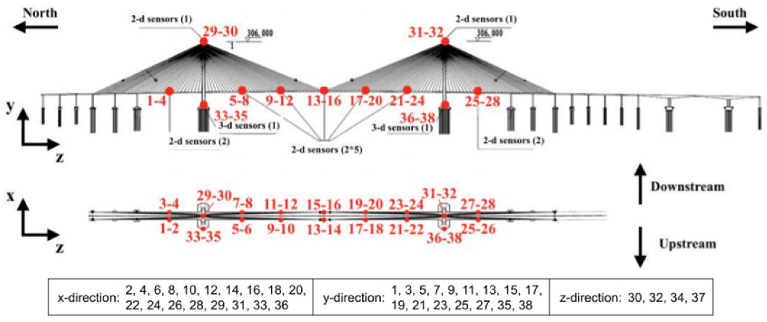
2.1. Bridge Overview and Data Set Composition

This research uses the health monitoring data set of a large-span cable-stayed bridge in China. The main span of the bridge is 1088 m long, and the two side spans are 300 m each, including two 306 m-high towers. The structural health monitoring system of the bridge consists of 38 sensors. The position on the bridge is shown in Figure 1. Sensors include accelerometers, anemometers, strain gauges, global positioning systems (GPS), and thermometers. For this research, one-month (1 January–31 January 2012) acceleration data from all 38 sensors of the SHM system were used for data anomaly detection. The sampling frequency of the accelerometer is 20 Hz. The original continuous measurement data are divided into one-hour time periods, and in a one-month time period, through the method of non-overlapping windows, 744 time series measurement data of each sensor are obtained so as to obtain a total of 28,272 (744 × 38) data. The dimensions of a single data point are 1 × 72,000. Figure 2a–g shows an example of each type of data pattern. Table 1 describes the quantity and characteristics of normal data and six types of abnormal data. Each data point has a real category label. The normal time series measurement data are marked as 1, and the other six abnormal data patterns are marked as 2–7. It can be seen that nearly 52% of the data are abnormal. “Trend” is the main abnormal pattern that constitutes 20% of the data set, followed by “missing” and “square”, each accounting for about 10%. On the other hand, the “outlier” only accounts for 1.9% of the data set, followed by “drift”, which accounts for 2.4% of the data

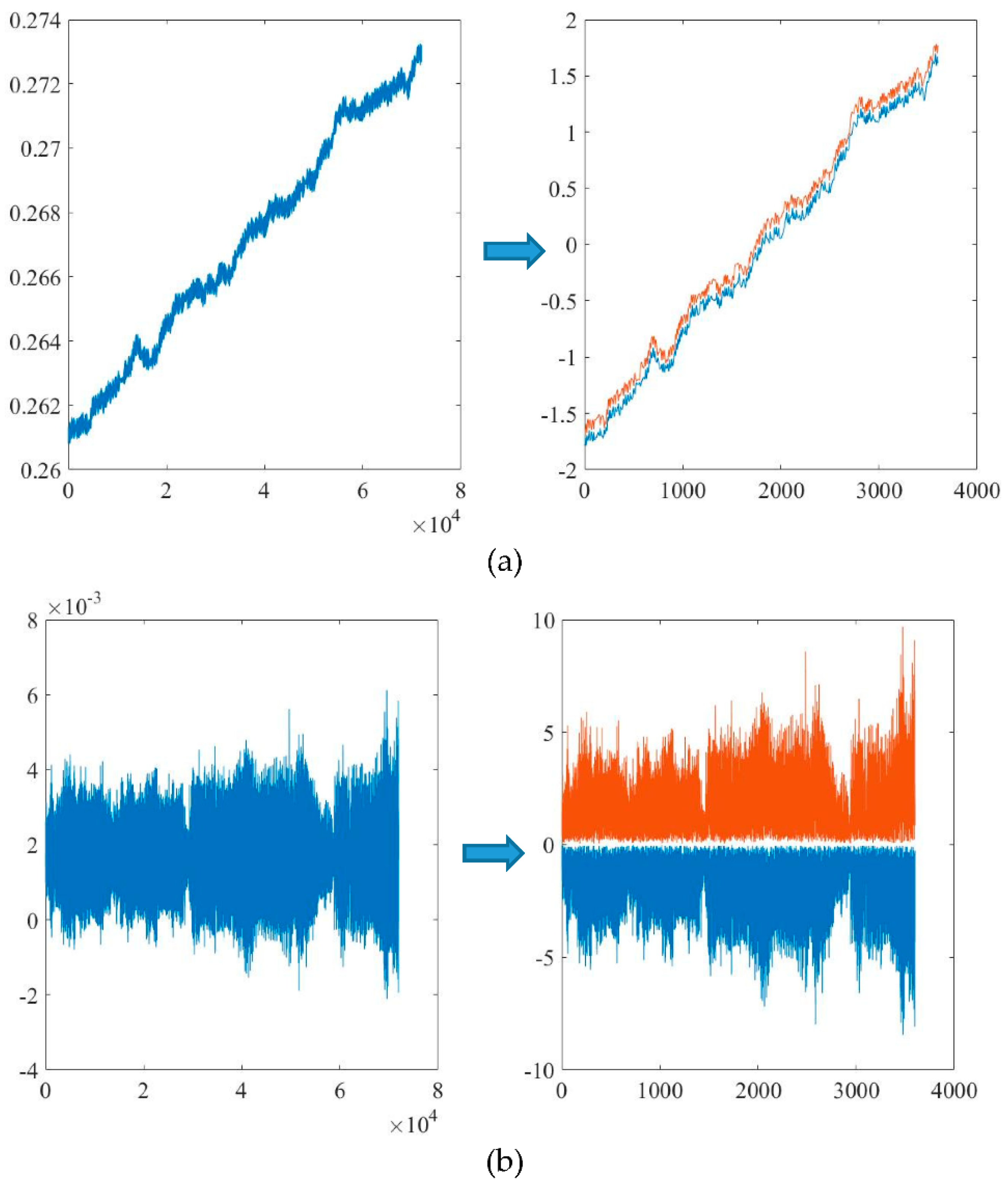
2.2. Data Preprocessing

Since there may be missing values or calculation errors in the process of data acquisition, data cleaning is performed on all data to remove missing or calculated incorrect values, which is reflected in MATLAB as “NAN”. In order to keep the data length unchanged as the input of the neural network, all “NAN” values are replaced with 0.
Zero-mean normalization is used to process the data for one hour so that the normalized data are normally distributed; that is, the mean is zero, and the standard deviation is one. This method can eliminate errors caused by self-variation or large differences in values, making the data more beneficial for subsequent steps. As shown in Equation (1),
x * = x μ σ
Where x is a one-hour time series {x1, x2, …, xN}, μ is the mean of all sampling points, σ is the standard deviation of all sampling points, and x* is the normalized time series.

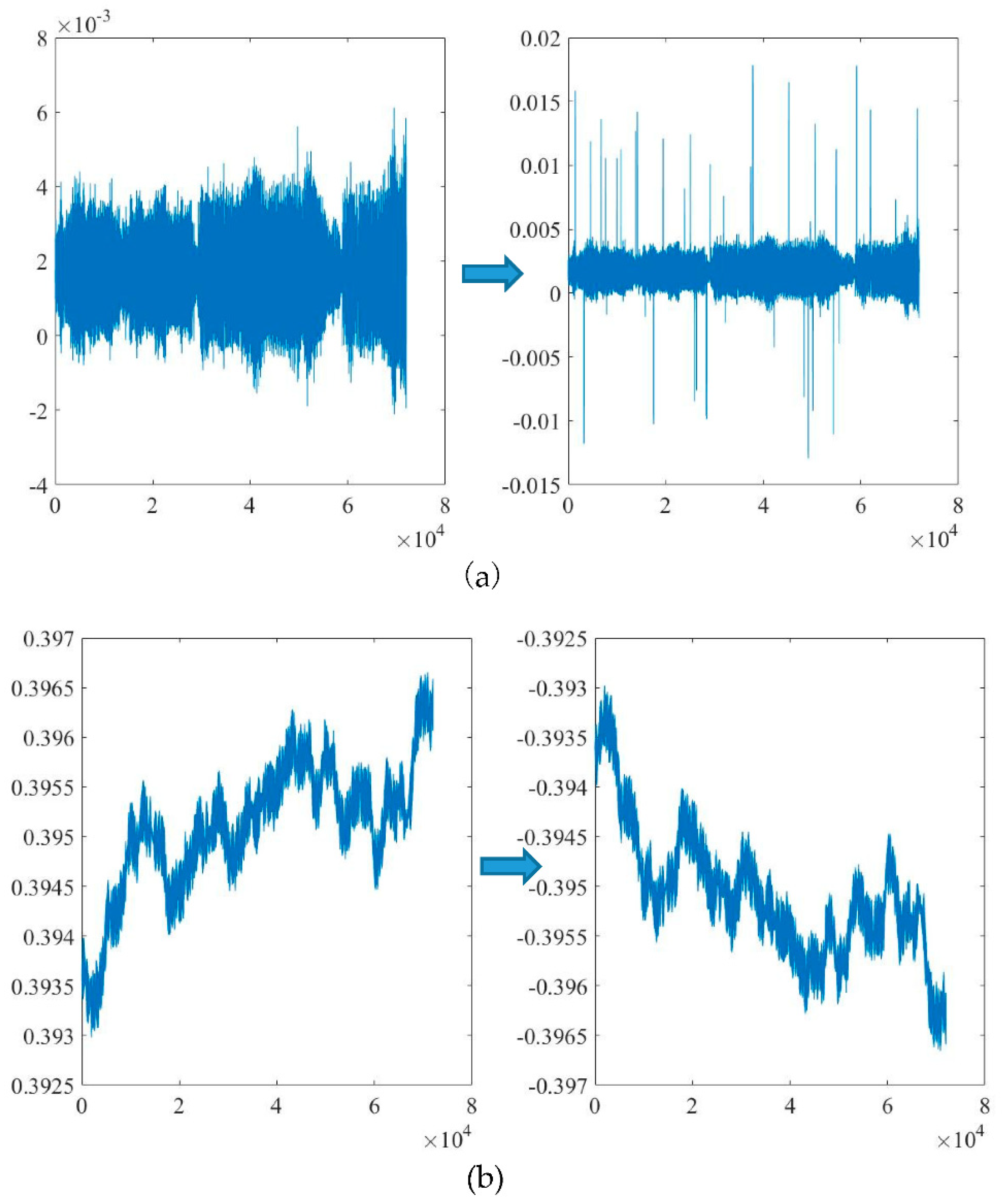
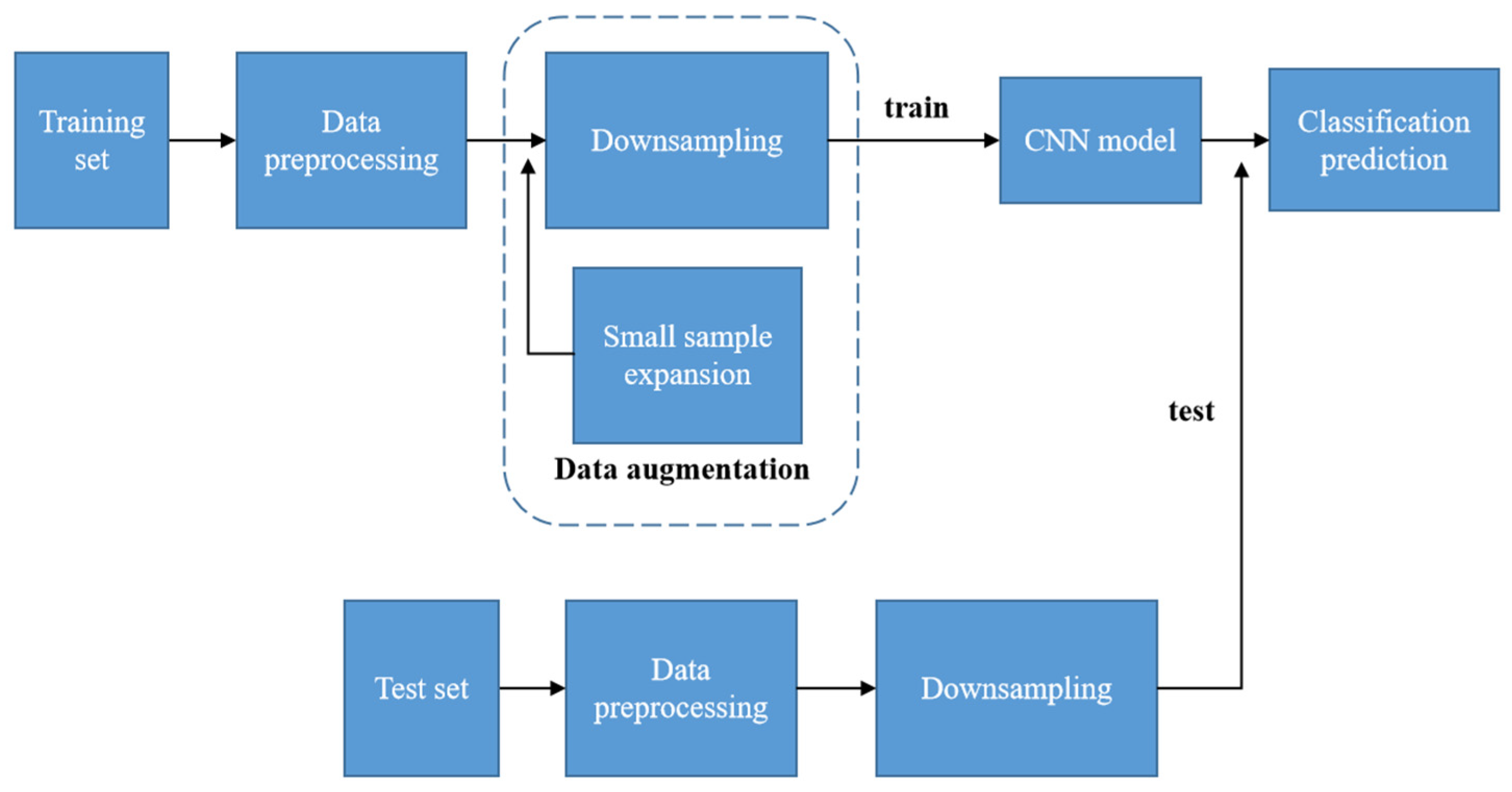
2.3. Data Augmentation
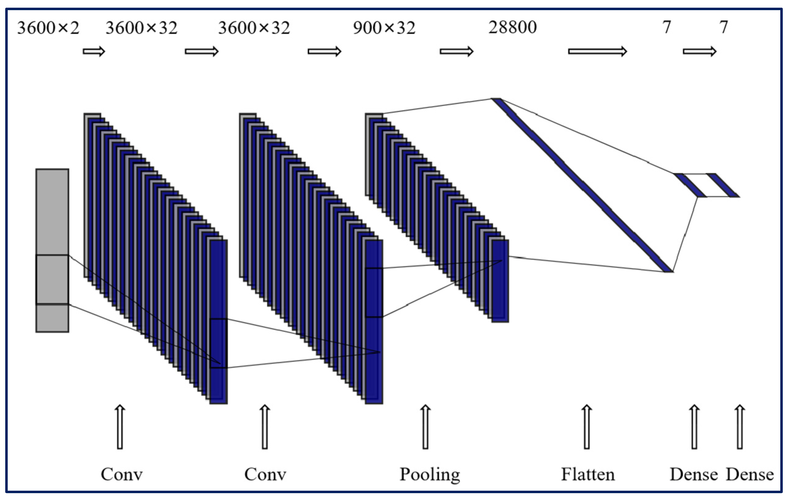
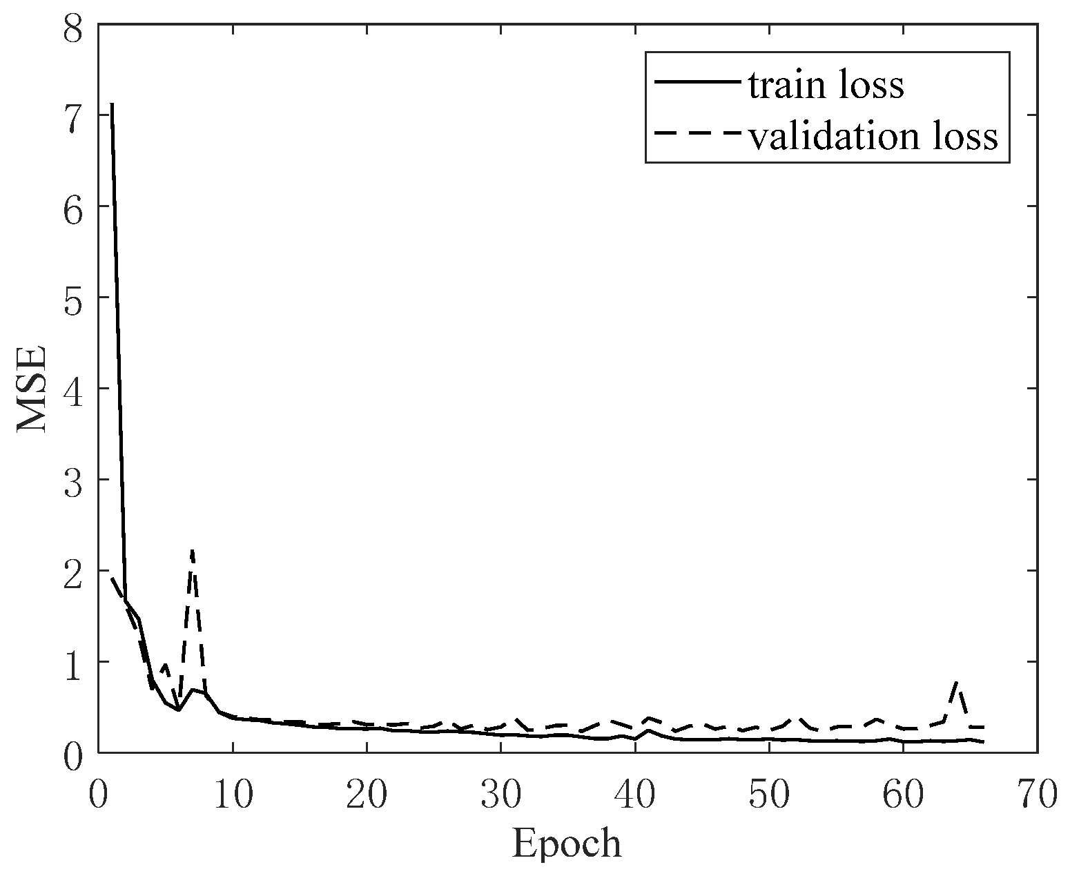
Augmentation methods should always be selected appropriately for the case under consideration [14]. For example, when applied to a time series containing outliers, the sliding window may not be able to capture the mutation features. Therefore, this research deals with every hour, that is, the full length of the sample.
Data enhancement includes two steps: data expansion of a small number of data samples and down-sampling of all samples.
Data expansion is applied to a small number of samples, namely outlier and drift, in the numerical simulation. Not all abnormal samples need to be expanded.
Outlier data can be defined as individual points of the normal data whose amplitude greatly exceeds the normal range. Therefore, a data expansion method that magnifies individual points is used for outlier samples. x is a normal sample {x1, x2, …, xN}, and the proposed method is shown in Equation (2),
x ( p ) = m e a n + β × r a n g e
where p is a random number between 10 and 60, mean is the mean value of x, β is a random number between −2 and 2, and range is the difference between the maximum and minimum values in x.
The method of symmetrical flipping and noise addition is used to expand the data of drift samples. The drift data has a random drift upwards or downwards. Therefore, the method of up-and-down symmetrical flipping can construct an effective sample. For the time series {x1, x2, …, xN}, symmetrical flipping can generate a new time series { x 1 , x 2 , , x N } with the same anomaly labels where x i = - x i . Different degrees of Gaussian white noise are added to the original sequence to generate more samples with the same anomaly labels. Two examples of data expansion are shown in Figure 3. The horizontal axis represents the number of sampling points, and the vertical axis represents the acceleration amplitude in m/s2.
The sample dimension of a single hour is 1 × 72,000, which is relatively large as the input of the neural network. Therefore, down-sampling is used to reduce the dimensionality of the sample while retaining the characteristics of the sample as much as possible to increase the efficiency of the neural network. The upper and lower contours of a sample are both useful features. Therefore, a down-sampling method that uses a sliding window to symmetrically extract the maxi-mum and minimum values is used. All 1 × 72,000 samples are down-sampled over the entire sample length. A step size is selected, which is 20 in this article, and the maximum and minimum values in the sequence are taken out for every sampling point of the step size. Therefore, after processing each of the 72,000 samples, a 2 × 3600 sample size will be obtained. The comparison chart of some examples before and after down-sampling is shown in Figure 4a,b. The horizontal axis represents the number of sampling points, and the vertical axis represents the acceleration amplitude in m/s2.

2.4. 1D-CNN

A convolutional neural network (CNN) usually consists of an input layer, convolutional layer (Conv), pooling layer (Pooling), dense layer (Dense), and output layer. In the CNN architecture, the first few layers usually alternate between convolutional layers and pooling layers, and the last few layers close to the output layer are composed of dense layers. CNN is an end-to-end learning method model, which can use the existing supervised gradient descent algorithm to train the model. For time-series-processing problems, the effect of a one-dimensional convolutional neural network (1D-CNN) can be comparable to a recurrent neural network (RNN), and the computational cost is much smaller. For simple tasks such as time series classification, a small one-dimensional convolutional network can completely replace the RNN, and it runs faster [21].
Regardless of whether one-dimensional or two-dimensional convolution is used, convolutional neural networks have a similar structure. The structure starts with a stack of convolutional and pooling layers, and then connected to a flatten layer to convert two-dimensional features into one-dimensional output, and then multiple dense layers can be added for classification or regression. However, there is a little difference between them: one-dimensional convolutional neural networks can use larger convolution kernels [21]. For example, for a two-dimensional convolution layer, a 3 × 3 convolution kernel contains 3 × 3 = 9 convolution vectors; however, for a one-dimensional convolution layer, a convolution kernel of size 3 only contains 3 convolution vectors. Therefore, a one-dimensional convolution kernel greater than or equal to 9 can be easily used.
The Python Science Suite, Tensorflow, and Keras are used to build a neural network architecture with GPU acceleration. The processor and graphics card types of the hardware platform are Inter Core i5-9400F and Nvidia GeForce RTX 2070. The object function in CNN is set to categorical cross-entropy to estimate the difference between the actual data category and the predicted data category. The metric is set to the accuracy to evaluate the performance of the model. In order to minimize the output of the object function, an adaptation of the mini-batch stochastic gradient descent algorithm called Adam is used as an optimizer.
In the classification, the imbalanced training set needs to be considered; that is, the number of normal samples is much larger than the abnormal samples. If an imbalanced training set is used to train the network, all abnormal samples will be predicted as normal samples during the test, and there will still be a high accuracy, but this is meaningless. Therefore, we choose to use the class weight technique [22], which can make important categories of samples contribute more to the object function during training. Batch Normalization (BN) [23,24] is a method that has been widely used in deep network training. The method of adding BN after the convolutional layer and then adding the activation function can save the operator from adjusting the parameters deliberately and slowly. Figure 5 shows the workflow of the proposed method.

3. Bridge Monitoring Data Verification

According to the proposed method process, anomaly detection is performed on the bridge monitoring data set. First, data preprocessing is performed on all original samples, missing values are deleted, and samples are standardized. In order to test the generalization ability of the model, the data set is divided into training and test sets, and 80% of the samples are randomly selected as the training set. The training set size is 22,616. Twenty percent of the samples are randomly selected as the test set, and the test set size is 5656. In order to simulate real anomalies, the distribution of test samples is unbalanced. Table 2 shows the distribution of selected test samples.
Constructing a balanced training set of various categories is beneficial to the training process. Data expansion is carried out on the small number of anomalies in the training set, namely outlier and drift. The normal samples in all training sets are expanded to outlier samples by magnifying individual points. The Gaussian distributed noise with 2%, 3%, 4%, 5%, 6%, 7%, and 8% standard deviation to the signals are added to each drift sample once, and symmetrical flip it once to obtain 8 times the number of drift samples. Therefore, an additional 10,860 (13,575 × 80%) outlier samples and 4345 (679 × 80% × 8) drift samples were obtained. After adding to the training set, the new training set size is 37,821 (22,616 + 10,860 + 4345).
Down-sampling is implemented on the test set and new training set samples, and the dimensionality of the samples is reduced from 1 × 72,000 to 2 × 3600 while retaining most of their features.
In order to build the 1D-CNN architecture, two one-dimensional convolutional layers are stacked to obtain the deep features of the sample more efficiently, and a flatten layer and two dense layers are connected to convert two-dimensional features into one-dimensional output. The last layer of the network uses the softmax multi-classifier. In short, softmax is the value that maps the output of the previous layer to (0,1) through the softmax function. The sum of these values is 1, which can be understood as a probability. The node with the largest probability is selected as the predicted abnormal data type. The network structure is shown in Figure 6. The detailed structure of 1D-CNN is shown in Table 3. The hyperparameter configuration is shown in Table 4.
Mean Squared Error (MSE) as a loss function for training and validation can be expressed as:
M S E = 1 N i = 1 N ( Y i Y 0 , i ) 2  
where Y represents the predicted value, and Y0 represents the true label value. N represents the total number of samples.
In the training process, the training set is divided into 12.5% as the verification set. During the training process, the training loss and the validation loss (MSE) are monitored, and the training accuracy and verification accuracy (Accuracy) are also monitored. The change of the loss function and the change of the accuracy are shown in Figure 7 and Figure 8.
It can be seen that the overall loss value shows a downward trend, and the overall accuracy shows an upward trend. The amplitude is large at the beginning of training, indicating that the learning rate is appropriate. There are glitches and oscillations locally, possibly because a large batch size is selected for a large number of samples, and there are a small number of samples with incorrect labels in the real-world data set. After the loss value and accuracy stabilized, the final training and validation accuracy reached more than 95%.
Table 5 shows the classification results in a statistical way. In the statistical analysis of binary or multiple classifications, precision, recall, and F1 score are measures of the accuracy of the classification results, and the last one is the harmonic average of the first two. Recall is relative to the sample, that is, how many positive samples in the sample are predicted correctly. Take the missing-type samples in Table 5 as an example. There are a total of 603 missing-type samples. If 602 are predicted correctly, the recall is 602/603 = 99.83%. Precision is relative to the prediction result. It indicates how many of the samples whose predictions are positive are correct. Taking the normal-type samples as an example, a total of 2590 samples are predicted to be normal types. If 2542 predictions are correct, the precision is 2542/2590 = 98.15%. Recall and precision indicators are sometimes contradictory. If a comprehensive indicator is used to express the results of recall and precision, the most common method should be the F1 score as follows:
F 1 = 2 p r e c i s i o n r e c a l l p r e c i s i o n + r e c a l l × 100 %
Where F1 represents F1 score, recall represents recall, and precision represents precision.
It can be seen that the proposed method can effectively identify various data patterns. The recall of normal, missing, minor, square, trend, and drift categories can reach above 90%. Except for the low F1 score of outlier and drift, the other types are all high. A small number of minor samples are classified into the normal category. Some outlier samples are classified into the normal category, and a few are classified into the minor category. The outlier sample may have only a few peaks, and most of the features of the outlier sample are very similar to the normal sample, and the feature that is too small will be lost in the convolution process. Trend and drift are partly confused, probably because they both have slanted features.

4. Conclusions

This paper modeled the anomaly detection problem into a time series classification problem. The original time series undergoes data preprocessing and data augmentation to get a sample set with more uniform distribution, more obvious features, and smaller dimensions. Data augmentation includes data expansion and down-sampling. For small samples, the methods of symmetrical flipping, adding noise, and randomly generating outliers are used for data expansion, and samples with the same label are added without increasing the original samples. The down-sampling method of symmetrically extracting the maximum and minimum values can effectively reduce the dimensionality of the input sample and retain its features. Build a one-dimensional convolutional neural network model that is faster for time series classification problems. Adding the hyperparameter tuning of class weights makes the network more effective in dealing with an unbalanced training set. The method is verified with the acceleration data of a long-span cable-stayed bridge for one month. For the anomaly detection problem modeled as a time series classification problem, the results show that the proposed method can automatically detect a variety of data anomaly categories with high precision.
The proposed method can accurately identify most types of abnormal data, but for abnormal types with very inconspicuous features, such as outlier data, there is still much room for improvement in recognition accuracy. In future work, time series augmentation will not only be carried out in the time domain, but will be expanded to the frequency domain, or more advanced methods (such as GAN) will be used to expand samples.

Author Contributions

Conceptualization, Y.Z. and Y.L.; methodology, Y.Z.; validation, Y.Z. and Y.L.; investigation, Y.Z.; data curation, Y.Z.; writing—original draft preparation, Y.Z.; writing—review and editing, Y.L.; funding acquisition, Y.L. All authors have read and agreed to the published version of the manuscript.

Funding

This research was funded by the National Key R&D Program of China via Grant No. 2018YFC0705606.

Institutional Review Board Statement

Not applicable.

Informed Consent Statement

Not applicable.

Data Availability Statement

Restrictions apply to the availability of these data. Data was obtained from The 1st International Project Competition for Structural Health Monitoring with the permission of The 1st International Project Competition for Structural Health Monitoring organizing committee.

Acknowledgments

The raw data involved in this study were obtained from the organizing committee of the 1st International Project Competition for Structural Health Monitoring (IPC-SHM (2020)), and the authors thank IPC-SHM (2020) organizing committee for its valuable data resources.

Conflicts of Interest

The authors declare no conflict of interest.

References

  1. Yi, T.H.; Huang, H.B.; Li, H.N. Development of sensor validation methodologies for structural health monitoring: A comprehensive review. Measurement 2017, 109, 200–214. [Google Scholar] [CrossRef]
  2. Chang, C.M.; Chou, J.Y. Damage detection of seismically excited buildings based on prediction errors. J. Aerosp. Eng. 2018, 31, 04018032.1–04018032.9. [Google Scholar] [CrossRef]
  3. Kang, F.; Li, J.; Dai, J. Prediction of long-term temperature effect in structural health monitoring of concrete dams using support vector machines with jaya optimizer and salp swarm algorithms. Adv. Eng. Softw. 2019, 131, 60–76. [Google Scholar] [CrossRef]
  4. Moriot, J.; Quaegebeur, N.; Le Duff, A.; Masson, P. A model-based approach for statistical assessment of detection and localization performance of guided wave-based imaging techniques. Struct. Health Monit. 2017, 17, 1460–1472. [Google Scholar] [CrossRef] [Green Version]
  5. Wang, H.; Zhang, Y.M.; Mao, J.X.; Wan, H.P.; Tao, T.Y.; Zhu, Q.X. Modeling and forecasting of temperature-induced strain of a long-span bridge using an improved bayesian dynamic linear model. Eng. Struct. 2019, 192, 220–232. [Google Scholar] [CrossRef]
  6. Chandola, V.; Banerjee, A.; Kumar, V. Anomaly detection: A survey. ACM Comput. Surv. 2009, 41, 15. [Google Scholar] [CrossRef]
  7. Xu, B.; He, J.; Masri, S.F. Data-based model-free hysteretic restoring force and mass identification for dynamic systems. Comput. Aided Civ. Infrastruct. Eng. 2015, 30, 2–18. [Google Scholar] [CrossRef]
  8. Fawaz, H.I.; Forestier, G.; Weber, J.; Idoumghar, L.; Muller, P.A. Deep learning for time series classification: A review. Data Min. Knowl. Discov. 2019, 33, 917–963. [Google Scholar] [CrossRef] [Green Version]
  9. Han, Z.; Zhao, J.; Leung, H.; Ma, K.F.; Wang, W. A review of deep learning models for time series prediction. IEEE Sens. J. 2019, 21, 7833–7848. [Google Scholar] [CrossRef]
  10. Chalapathy, R.; Chawla, S. Deep learning for anomaly detection: A survey. arXiv 2019, arXiv:1901.03407. [Google Scholar]
  11. Bao, Y.; Tang, Z.; Li, H.; Zhang, Y. Computer vision and deep learning-based data anomaly detection method for structural health monitoring. Struct. Health Monit. 2019, 18, 401–421. [Google Scholar] [CrossRef]
  12. Tang, Z.; Chen, Z.; Bao, Y.; Li, H. Convolutional neural network-based data anomaly detection method using multiple information for structural health monitoring. Struct. Control. Health Monit. 2018, 26, e2296. [Google Scholar] [CrossRef] [Green Version]
  13. Mao, J.; Wang, H.; Spencer, B.F. Toward data anomaly detection for automated structural health monitoring: Exploiting generative adversarial nets and autoencoders. Struct. Health Monit. 2020. [Google Scholar] [CrossRef]
  14. Wen, Q.; Sun, L.; Song, X.; Gao, J.; Wang, X.; Xu, H. Time series data augmentation for deep learning: A survey. arXiv 2020, arXiv:2002.12478v1. [Google Scholar]
  15. Sun, J.; Wang, M.T.; Zhao, X.; Zhang, D.J. Multi-View Pose Generator Based on Deep Learning for Monocular 3D Human Pose Estimation. Symmetry 2020, 12, 1116. [Google Scholar] [CrossRef]
  16. Liu, B.; Zhang, Y.; He, D.J.; Li, Y.X. Identification of Apple Leaf Diseases Based on Deep Convolutional Neural Networks. Symmetry 2018, 10, 11. [Google Scholar] [CrossRef] [Green Version]
  17. Cui, Z.; Chen, W.; Chen, Y. Multi-scale convolutional neural networks for time series classification. arXiv 2016, arXiv:1603.06995. [Google Scholar]
  18. Fawaz, H.I.; Forestier, G.; Weber, J.; Idoumghar, L.; Muller, P.A. Data augmentation using synthetic data for time series clas-sification with deep residual networks. arXiv 2018, arXiv:1808.02455v1 [cs.CV]. [Google Scholar]
  19. Wen, T.; Keyes, R. Time series anomaly detection using convolutional neural networks and transfer learning. arXiv 2019, arXiv:1905.13628v1 [cs.LG]. [Google Scholar]
  20. Gao, J.; Song, X.; Wen, Q.; Wang, P.; Sun, L.; Xu, H. Robusttad: Robust time series anomaly detection via decomposition and convolutional neural networks. arXiv 2020, arXiv:2002.09535. [Google Scholar]
  21. Francois Chollet. Deep Learning with Python; Manning: New York, NY, USA, 2018; pp. 188–190. [Google Scholar]
  22. Keras. Available online: https://keras.io/ (accessed on 31 October 2019).
  23. Alom, M.Z.; Taha, T.M.; Yakopcic, C. A State-of-the-Art Survey on Deep Learning Theory and Architectures. Electronics 2019, 8, 292. [Google Scholar] [CrossRef] [Green Version]
  24. Lin, Y.; Nie, Z.; Ma, H. Structural Damage Detection with Automatic Feature-Extraction through Deep Learning. Comput. Aided Civ. Infrastruct. Eng. 2017, 32, 1025–1046. [Google Scholar] [CrossRef]
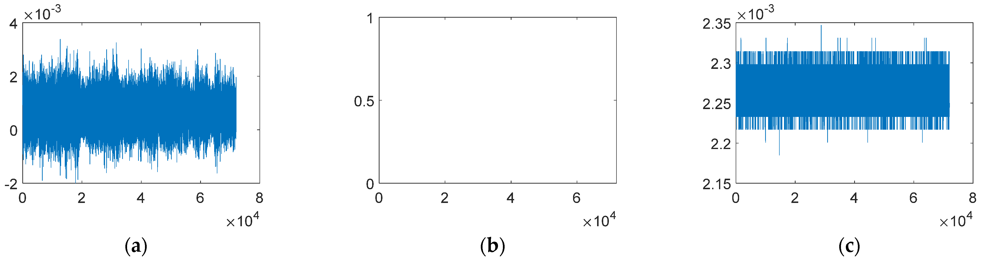
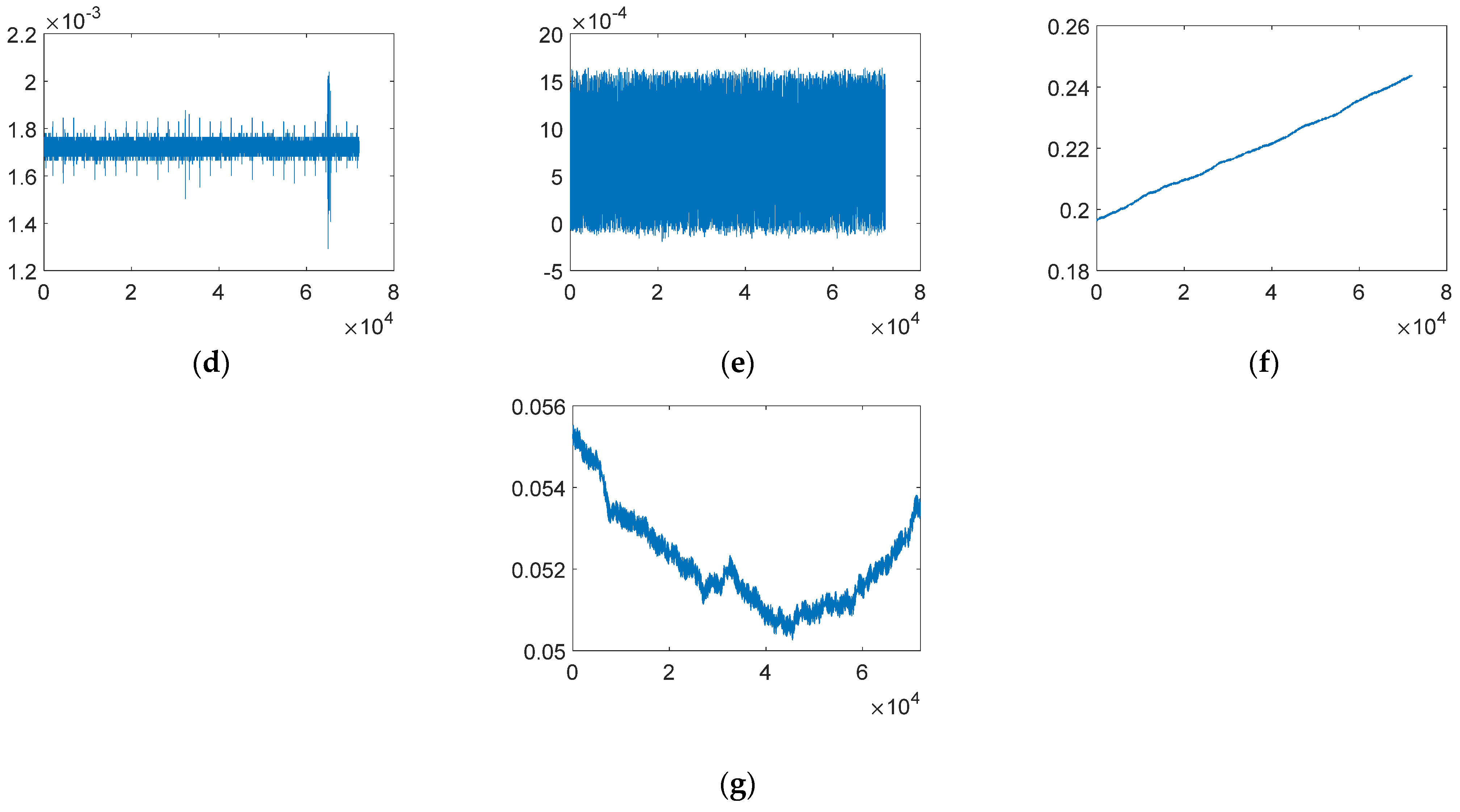
Figure 1. The monitored bridge and the position of the accelerometer on the bridge deck and tower. Source: The 1st International Project Competition for Structural Health Monitoring, July 2020.
Symmetry 13 01186 g001
Figure 2. The example for each data pattern. (a) Normal data; (b) Missing data; (c) Minor data; (d) Outlier data; (e) Square data; (f) Trend data; (g) Drift data.
Symmetry 13 01186 g002aSymmetry 13 01186 g002b
Figure 3. Comparison chart before and after data expansion. (a) Data expansion for outlier data; (b) Data expansion for drift data.
Symmetry 13 01186 g003
Figure 4. Before and after data preprocessing and down-sampling. (a) Preprocessing and down-sampling of trend data; (b) Preprocessing and down-sampling of normal data.
Symmetry 13 01186 g004
Figure 5. Workflow of the proposed method.
Symmetry 13 01186 g005
Figure 6. Schematic of the proposed CNN architecture.
Symmetry 13 01186 g006
Figure 7. Training and validation loss curve.
Symmetry 13 01186 g007
Figure 8. Training and validation accuracy curve.
Symmetry 13 01186 g008
Table 1. Description of each type of data pattern.
No.Anomaly
Patterns
DescriptionQuantity
1NormalThe time response is normal oscillation curve; frequency response is peak-like (may differ between bridges)13575
(48%)
2MissingMost/all of the time response is missing, which makes the time and frequency response zero2942
(10.4%)
3MinorRelative to normal sensor data, the amplitude is very small in the time domain1775
(6.3%)
4OutlierOne or more outliers appear in the time response527
(1.9%)
5SquareThe time response is like a square wave2996
(10.6%)
6TrendThe data has an obvious trend in the time domain and has an obvious peak value in the frequency domain5778
(20.4%)
7DriftThe vibration response is non-stationary, with random drift679
(2.4%)
Table 2. Data distribution of the test set.
1234567
Anomaly patternsNormalMissingMinorOutlierSquareTrendDrift
Quantity26886033601066161147136
Percentage47.5%10.7%6.4%1.9%10.9%20.3%2.4%
Table 3. The detailed architecture of CNN.
LayerTypeInput ShapeOutput ShapeKernel NumKernel SizeStridePaddingwith BNActivation
1Conv(3600, 2)(3600, 32)32161SameTrueLeaky ReLU
2Conv(3600, 32)(3600, 32)32161SameTrueLeaky ReLU
3Pooling(3600, 32)(900, 32)None44ValidFalseNone
4Flatten(900, 32)(28800)NoneNoneNoneNoneNoneNone
5Dense(28800)(7)NoneNoneNoneNoneFalseLeaky ReLU
6Dense(7)(7)NoneNoneNoneNoneFalseSoftmax
Table 4. The configurations of training process.
NameValueDescription
Batch size128The size of data batch used in every training iteration
Initial learning rate10−3The initial learning rate of Adam algorithm
Patience40A parameter of early stopping
α0.01A parameter in Leaky RELU function
0.01 in every activation function
Table 5. The prediction result of the test set.
Predicted Data Pattern
1234567TotalRecall (%)
Real data pattern1-normal2542060721400268894.57
2-missing06021000060399.83
3-minor260326800036090.56
4-outlier21018400010679.24
5-square10126120061699.35
6-trend00200111035114796.77
7-drift000001312313690.44
Total25906023911666261123158565695.45
Precision
(%)
98.15100.083.3850.6097.7698.8477.85
F1 score0.96 1.00 0.87 0.62 0.99 0.98 0.84
Publisher’s Note: MDPI stays neutral with regard to jurisdictional claims in published maps and institutional affiliations.

