Effect of Plastic Anisotropy on the Collapse of a Hollow Disk under Thermal and Mechanical Loading

Abstract

Plastic anisotropy significantly affects the behavior of structures and machine parts. Given the many parameters that classify a structure made of anisotropic material, analytic and semi-analytic solutions are very useful for parametric analysis and preliminary design of such structures. The present paper is devoted to describing the plastic collapse of a thin orthotropic hollow disk inserted into a rigid container. The disk is subject to a uniform temperature field and a uniform pressure is applied over its inner radius. The condition of axial symmetry in conjunction with the assumption of plane stress, permits an exact analytic solution. Two plastic collapse mechanisms exist. One of these mechanisms requires that the entire disk is plastic. According to the other mechanism, plastic deformation localizes at the inner radius of the disk. Additionally, two special solutions are possible. One of these solutions predicts that the entire disk becomes plastic at the initiation of plastic yielding (i.e., plastic yielding simultaneously initiates in the entire disk). The other special solution predicts that the plastic localization occurs at the inner radius of the disk with no plastic region of finite size. An essential difference between the orthotropic and isotropic disks is that plastic yielding might initiate at the outer radius of the orthotropic disk.

1. Introduction

Elastic/plastic plane stress solutions attract considerable interest due to their capability to describe such important engineering structures and machine parts, as thin disks are subject to various types of loading, rotating disks, and open-ended cylinders. A review of solutions for thin hollow disks subject to thermomechanical loading is provided in [1]. The recent study [2] analyzed the available solutions for rotating disks. Several numerical codes were developed to specifically deal with plane stress problems [3,4,5,6,7]. It was noted in [5] that the application of computational models to plane stress problems leads to specific difficulties that are non-existent in other formulations. On the other hand, closed-form solutions, when available, are more computationally efficient than FEM and other numerical solutions [8,9]. Therefore, an analytic method is used in the present study.

Plastic anisotropy is a common property of many metallic materials. It is known that even mild plastic anisotropy significantly affects some features of elastic/plastic solutions [10]. It is, therefore, crucial to study the effect of elastic and plastic anisotropy on the solution behavior for various structures and machine parts. Several solutions for polar orthotropic rotating disks were proposed in [11,12,13,14]. Some studies [11,12,14] deal with elastic anisotropy. Another study [11] emphasizes the influence of orthotropy and gradient on the elastic stress and strain field, especially the circumferential stress distribution, in hollow annular plates rotating at a constant angular speed about its axis. The closed-form expressions were found for the gradient of power–law profiles. In [12], analytical plane stress solutions were developed for polar orthotropic functionally graded annular disks, rotating with a constant angular velocity. A non-linear function involving three parameters, controls the radial variation of the elasticity moduli and thickness. No restriction is imposed on the radial variation of density. Poisson’s ratio is constant. Uniform rotating discs made of radial, functionally graded polar orthotropic materials were studied in [14], using both analytical and numerical methods. Several possible boundary conditions and frequently used distributions of materials properties were adopted. The complementary functions method was used as a numerical technique to solve the governing equation with variable coefficients. Study [13] emphasizes the importance of accounting for plastic anisotropy in elastic/plastic solutions, for thin rotating disks.

A thin disk inserted into a rigid container and subject to simultaneous loading by a uniform pressure over its inner radius and a uniform temperature field, was studied in [15,16]. Another study [15] deals with an elastic, perfectly plastic model of pressure-independent plasticity. This paper revealed several qualitative features of the solution at plastic collapse. In particular, two plastic collapse mechanisms were identified. According to one of these mechanisms, the entire disk becomes plastic. The other mechanism predicts the localization of plastic deformation at the inner radius of the disk. Such solution behavior in the vicinity of holes was first discovered in [17], for an isotropic rigid/plastic model. This phenomenon was further investigated in [18] for an isotropic elastic/plastic model. A particular case of the boundary value problem considered in [15,16] with no mechanical loading was solved in [19], assuming temperature-dependent material properties. It was found that the magnitude of plastic strain at plastic collapse is very small, which justifies adopting the perfectly plastic models.

The present study extends the formulation of the boundary value problem in [15,16] to include plastic anisotropy. It was assumed that the disk was polar orthotropic. Hill’s quadratic yield criterion was adopted [17]. The solution was semi-analytic. A numerical technique was only necessary to solve transcendent equations.

2. Statement of the Problem

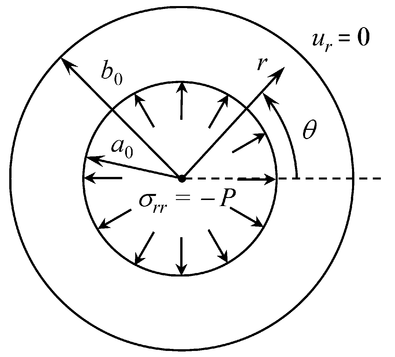
A thin hollow disk of outer radius $b_0$ and inner radius $a_0$ was inserted into a rigid container of radius $b_0$. The disk was subject to a uniform temperature field T and pressure P was uniformly distributed over its inner radius (Figure 1). Here, T was the increase in temperature from its reference value. It is natural to use a cylindrical coordinate system $\left(r,\hspace{0.17em}\theta ,\hspace{0.17em}z\right)$ whose z-axis coincides with the disk’s axis of symmetry. Let ${\sigma }_r$, ${\sigma }_{\theta }$, and ${\sigma }_z$ be the normal stresses referred to this coordinate system. These stresses are the principal stresses. Moreover, the state of stress was plane, ${\sigma }_z=0$. The stress boundary condition was:

$${\sigma }_r=-P \mathrm{for} r=a_0.$$

(1)

Since the container was rigid, the displacement boundary condition was

$$u_r=0 \mathrm{for} r=b_0.$$

(2)

Here, $u_r$ is the radial displacement. The circumferential displacement vanished.

Let ${\epsilon }_r$, ${\epsilon }_{\theta }$, and ${\epsilon }_z$ be the total normal strains referred to the cylindrical coordinate system. The classical Duhamel–Neumann law was adopted in the elastic region. In the case under consideration, this law reduced to:

$${\epsilon }_r^{}=\frac{{\sigma }_r-\nu {\sigma }_{\theta }}{E}+\alpha T,\hspace{1em}{\epsilon }_{\theta }^{}=\frac{{\sigma }_{\theta }-\nu {\sigma }_r}{E}+\alpha T, \mathrm{and} {\epsilon }_z^{}=-\frac{\nu \left({\sigma }_r+{\sigma }_{\theta }\right)}{E}+\alpha T.$$

(3)

Here, $E$ is Young’s modulus, $\nu$ is Poisson’s ratio, and $\alpha$ is the thermal coefficient of linear expansion. Hill’s quadratic yield criterion [17] was adopted in the plastic region, assuming that the anisotropy’s principal axes coincide with the cylindrical coordinate system’s coordinate curves. In the case under consideration, this criterion becomes [1]:

$${\sigma }_r^2+{\left(\frac{{\sigma }_{\theta }}{{\eta }_1}\right)}^2-\frac{\eta }{{\eta }_1}{\sigma }_{\theta }{\sigma }_r={\sigma }_0^2.$$

(4)

Here, $\eta$, ${\eta }_1$, and ${\sigma }_0$ are expressible through the yield stresses, with respect to the principal axes of anisotropy. In particular [20],

$$\eta =XY\left(\frac{1}{X^2}+\frac{1}{Y^2}-\frac{1}{Z^2}\right),{\eta }_1=\frac{Y}{X}, \mathrm{and} {\sigma }_0=X$$

where X, Y, and Z are the yield stresses in the r-, $\theta -$ and z-directions, respectively.

In the case of traditional metallic materials,

$$\eta {\eta }_1<2.$$

(5)

In what follows, it was assumed that this inequality was satisfied. No other constitutive equations were required in the plastic region. The only equilibrium equation that was not satisfied automatically was:

$$\frac{\partial {\sigma }_r}{\partial r}+\frac{{\sigma }_r-{\sigma }_{\theta }}{r}=0.$$

(6)

It was convenient to introduce the following dimensionless quantities:

$$\rho =\frac{r}{b_0},\hspace{1em}\tau =\frac{\alpha TE}{{\sigma }_0},\hspace{1em}p=\frac{P}{{\sigma }_0}, \mathrm{and} a=\frac{a_0}{b_0}.$$

(7)

Then, the boundary conditions (1) and (2) become:

$$\frac{{\sigma }_r}{{\sigma }_0}=-p \mathrm{for} \rho =a$$

(8)

And,

$$u_r=0 \mathrm{for} \rho =1,$$

(9)

respectively.

3. Purely Elastic Solution and the Initiation of Plastic Yielding

The purely elastic solution is well-known [1]. Using (7), one can represent this solution as:

$$\frac{{\sigma }_r}{{\sigma }_0}=\frac{A}{{\rho }^2}+B,\hspace{1em}\frac{{\sigma }_{\theta }}{{\sigma }_0}=-\frac{A}{{\rho }^2}+B,\hspace{1em}\frac{E}{{\sigma }_0}\frac{u_r}{a_0}=\left(1-\nu \right)B\rho -\left(1+\nu \right)\frac{A}{\rho }+\tau \rho .$$

(10)

where A and B are constant. The boundary conditions (8) and (9) require that

$$A=A_e=\frac{a^2\left[\tau -p\left(1-\nu \right)\right]}{\left(1+\nu \right)a^2+1-\nu },\hspace{1em}B=B_e=-\frac{\tau +p{a}^2\left(1+\nu \right)}{\left(1+\nu \right)a^2+1-\nu }.$$

(11)

It is worthy of note that the stress components were independent of $\rho$, if $A=0$. It follows from (10) and (11), that:

$$\frac{{\sigma }_r}{{\sigma }_0}=\frac{{\sigma }_{\theta }}{{\sigma }_0}=-p$$

(12)

if

$$\tau -p\left(1-\nu \right)=0.$$

(13)

Plastic yielding could initiate at $\rho =a$ or $\rho =1$. Substituting (10) and (11) at $\rho =a$ into (4), gives the following:

$$\frac{{\left\{\left[\nu -1+a^2\left(1+\nu \right)\right]p+2\tau \right\}}^2}{{\eta }_1^2{\left[1-\nu +a^2\left(1+\nu \right)\right]}^2}-\frac{\eta p\left\{\left[\nu -1+a^2\left(1+\nu \right)\right]p+2\tau \right\}}{{\eta }_1\left[1-\nu +a^2\left(1+\nu \right)\right]}+p^2-1=0.$$

(14)

This equation determined the interdependence of p and $\tau$, corresponding to the initiation of plastic yielding at the inner radius of the disk. Substituting (10) and (11) at $\rho =1$ into (4), gives:

$$\begin{array}{l}{a}^4{\left[\tau -p\left(1-\nu \right)\right]}^2\left(1+\frac{1}{{\eta }_1^2}+\frac{\eta }{{\eta }_1}\right)+{\left[\tau +p{a}^2\left(1+\nu \right)\right]}^2\left(1+\frac{1}{{\eta }_1^2}-\frac{\eta }{{\eta }_1}\right)-\\ 2a^2\left[\tau -p\left(1-\nu \right)\right]\left[\tau +p{a}^2\left(1+\nu \right)\right]\left(1-\frac{1}{{\eta }_1^2}\right)-{\left[\left(1+\nu \right)a^2+1-\nu \right]}^2=0.\end{array}$$

(15)

This equation determined the dependence between p and $\tau$ corresponding to the initiation of plastic yielding at the outer radius of the disk.

The plastic collapse solution below was based on the assumption that the plastic yielding was initiated at the inner radius of the disk.

4. Plastic Collapse

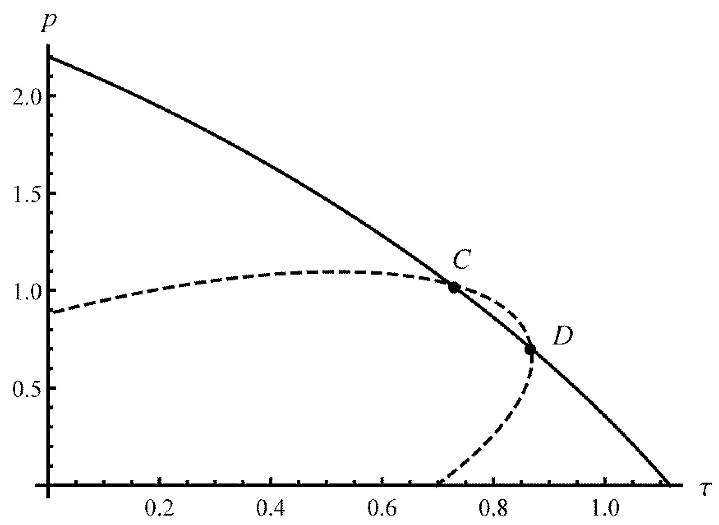
It is shown below that there are two plastic collapse mechanisms and two special solutions. The geometric interpretation of the general structure of the solution is shown in Figure 2 to simplify its further discussion. Curve CDEF represents Equation (14). It encompasses the region where the loading paths are purely elastic. Point C corresponds to the purely mechanical loading and point F to the purely thermal loading. The p-coordinate of the former is determined from (14) where one should put $\tau =0$, and the $\tau$-coordinate of the latter from the same equation where one should put $p=0$.

The yield criterion (4) is satisfied by the following substitution [1]:

$$\frac{{\sigma }_r}{{\sigma }_0}=-\frac{2\sin \psi }{\sqrt{4-{\eta }^2}} \mathrm{and} \frac{{\sigma }_{\theta }}{{\sigma }_0}=-{\eta }_1\left(\frac{\eta \sin \psi }{\sqrt{4-{\eta }^2}}+\cos \psi \right).$$

(16)

Here, $\psi$ is a new arbitrary function of $\rho$. Substituting (16) into the equilibrium Equation (6), gives:

$$2\rho \frac{\partial \psi }{\partial \rho }={\eta }_1\sqrt{4-{\eta }^2}-\left(2-\eta {\eta }_1\right)\tan \psi .$$

(17)

It is worthy of note that this equation has a special solution $\psi ={\psi }_s$, where:

$$\tan {\psi }_s=\frac{{\eta }_1\sqrt{4-{\eta }^2}}{2-\eta {\eta }_1}.$$

(18)

In this case, it follows from (16) that the stress components are independent of $\rho$. The corresponding value of p is determined from the boundary condition (8) and (16), as

$$p_s=\frac{2\sin {\psi }_s}{\sqrt{4-{\eta }^2}}.$$

(19)

It is seen from (5), (18), and (19) that $0<{\psi }_s<\pi /2$. This inequality allows for determining the unique value of ${\psi }_s$ from (18). It follows from (13) and (19) that the solutions (12) and (16) at $\psi ={\psi }_s$ coincide, if:

$$\tau ={\tau }_s=\frac{2\left(1-\nu \right)\sin {\psi }_s}{\sqrt{4-{\eta }^2}}.$$

(20)

Thus, if $p=p_s$ and $\tau ={\tau }_s$, then the plastic region occupies the entire disk at the instant of plastic yielding initiation. Point E in Figure 2 represents this special solution. The straight line determined by Equation (13) passes through the origin of the $\left(p,\tau \right)$ coordinate system and point E.

One can rewrite Equation (17), as:

$$2\rho \cos \psi \frac{\partial \psi }{\partial \rho }={\eta }_1\sqrt{4-{\eta }^2}\cos \psi -\left(2-\eta {\eta }_1\right)\sin \psi .$$

(21)

The coefficient at the derivative vanishes if $\psi =\pi /2$. The general solution of Equation (21) can be represented as

$$\ln \left(\frac{\rho }{{\rho }_0}\right)=\frac{{\eta }_1\sqrt{4-{\eta }^2}\left(\psi -{\psi }_0\right)}{2\left(1+{\eta }_1^2-\eta {\eta }_1\right)}-\frac{\left(2-\eta {\eta }_1\right)}{2\left(1+{\eta }_1^2-\eta {\eta }_1\right)}\ln \left[\frac{{\eta }_1\sqrt{4-{\eta }^2}\cos \psi -\left(2-\eta {\eta }_1\right)\sin \psi }{{\eta }_1\sqrt{4-{\eta }^2}\cos {\psi }_0-\left(2-\eta {\eta }_1\right)\sin {\psi }_0}\right].$$

(22)

The solution in this form satisfies the condition $\psi ={\psi }_0$ for $\rho ={\rho }_0$. Considering ${\psi }_0=\pi /2$ here, leads to:

$$\ln \left(\frac{\rho }{{\rho }_0}\right)=\frac{{\eta }_1\sqrt{4-{\eta }^2}\left(\psi -\pi /2\right)}{2\left(1+{\eta }_1^2-\eta {\eta }_1\right)}-\frac{\left(2-\eta {\eta }_1\right)}{2\left(1+{\eta }_1^2-\eta {\eta }_1\right)}\ln \left[\sin \psi -\frac{{\eta }_1\sqrt{4-{\eta }^2}}{\left(2-\eta {\eta }_1\right)}\cos \psi \right].$$

(23)

Expanding the right-hand side of this equation in a series in the vicinity of $\psi =\pi /2$ gives:

$$\frac{\rho }{{\rho }_0}=1+\frac{{\left(\pi /2-\psi \right)}^2}{\left(2-\eta {\eta }_1\right)}+o\left[{\left(\pi /2-\psi \right)}^2\right]$$

(24)

as $\psi \to \pi /2$. This expansion and (5) shows that $\rho >{\rho }_0$ in the vicinity of $\psi =\pi /2$. This result contradicts the assumption that the plastic region propagates from the inner radius of the disk. Therefore, $\psi$ attains the value $\pi /2$, only if ${\rho }_0=a$ in (23). The solution breaks down at this instant. The physical interpretation of this collapse mechanism is that the localized thickening occurs at $\rho =a$ [17]. If $\psi =\pi /2$ at $\rho =a$ at the initiation of the plastic yielding, no plastic region of finite size develops at the plastic collapse. It is seen from (8) and (16) that this kind of plastic collapse occurs, if:

$$p=p_c=\frac{2}{\sqrt{4-{\eta }^2}}.$$

(25)

The corresponding value of $\tau$ is found from the following quadratic equation that results from the substitution of (25) into (14):

$${\tau }_c^2+\frac{\left[a^2\left(1+\nu \right)\left(2-\eta {\eta }_1\right)+\left(2+\eta {\eta }_1\right)\left(\nu -1\right)\right]}{\sqrt{4-{\eta }^2}}{\tau }_c+\frac{{\left[\left(2+\eta {\eta }_1\right)\left(\nu -1\right)+a^2\left(2-\eta {\eta }_1\right)\left(\nu +1\right)\right]}^2}{4\left(4-{\eta }^2\right)}=0.$$

(26)

Point D in Figure 2 represents this special solution.

The plastic collapse solutions above are special cases of two kinds of plastic collapse mechanisms. To simplify the further writing, PCM1 denotes the plastic collapse mechanism that occurs when the entire disk becomes plastic, and PCM2 is the plastic collapse mechanism that occurs when the localized thickening occurs at $\rho =a$. One of these plastic collapse mechanisms occurs in the general case. In the case of PCM2, Equation (25) is universal. Therefore, this plastic collapse mechanism is represented by a straight line parallel to the $\tau -$axis (line GJ in Figure 2). This line must contain point D. However, PCM1 can occur at a value of p that is smaller than $p_c$.

Let ${\psi }_0$ be the value of $\psi$ at $\rho =a$, at the initiation of plastic yielding. The stress components must be continuous across the elastic/plastic interface. Then, Equations (10), (11) and (16) combine to give:

$$p=\frac{2\sin {\psi }_0}{\sqrt{4-{\eta }^2}},\hspace{1em}\frac{2\tau +p\left[\left(1+\nu \right)a^2-1+\nu \right]}{\left(1+\nu \right)a^2+1-\nu }={\eta }_1\left(\frac{\eta \sin {\psi }_0}{\sqrt{4-{\eta }^2}}+\cos {\psi }_0\right).$$

(27)

These two equations represent the same curve as Equation (14) but in parametric form with ${\psi }_0$ being the parameter. One can eliminate p in the second Equation in (27) using the first equation. As a result,

$$\tau =\frac{\sin {\psi }_0}{\sqrt{4-{\eta }^2}}\left[a^2\left(1+\nu \right)\left(\frac{\eta {\eta }_1}{2}-1\right)+\left(1-\nu \right)\left(\frac{\eta {\eta }_1}{2}+1\right)\right]+\frac{cos{\psi }_0}{2}\left[a^2\left(1+\nu \right)+1-\nu \right]{\eta }_1.$$

(28)

Differentiating the first Equation in (27) and (28), one gets

$$\frac{dp}{d\tau }=4\cos {\psi }_0{\left\{\left[a^2\left(1+\nu \right)\left(\eta {\eta }_1-2\right)+\left(1-\nu \right)\left(\eta {\eta }_1+2\right)\right]\cos {\psi }_0-{\eta }_1\sqrt{4-{\eta }^2}\left[a^2\left(1+\nu \right)+1-\nu \right]\sin {\psi }_0\right\}}^{-1}.$$

(29)

It is seen from this equation that

$$\frac{dp}{d\tau }=0 \mathrm{at} {\psi }_0=\pi /2.$$

(30)

The second derivative is

$$\frac{d^{2}p}{d{\tau }^2}=\frac{d\left(dp/d\tau \right)/d{\psi }_0}{d\tau /d{\psi }_0}.$$

(31)

One can find from (28) that

$$\frac{d\tau }{d{\psi }_0}=-\frac{{\eta }_1}{2}\left[a^2\left(1+\nu \right)+1-\nu \right]$$

(32)

at ${\psi }_0=\pi /2$. Differentiating the right-hand side of (29) results in

$$\frac{d}{d{\psi }_0}\left(\frac{dp}{d\tau }\right)=\frac{4}{{\eta }_1\sqrt{4-{\eta }^2}\left[a^2\left(1+\nu \right)+1-\nu \right]}$$

(33)

at ${\psi }_0=\pi /2$. It is evident from (31), (32) and (33) that $d^{2}p/d{\psi }_0^2<0$ at ${\psi }_0=\pi /2$. Therefore, p as a function of $\tau$, determined by (14), attains a local maximum at ${\psi }_0=\pi /2$. It was shown above that this point of the $\left(p\tau \right)$-space also belongs to the curve that represents PCM2. Therefore, if the loading path in the $p\tau$-space intersects the curve represented by (14) at $\tau \le {\tau }_c$ (arc CD in Figure 2), then PCM2 always occurs.

Consider the loading paths that intersect the curve represented by (14) at $\tau >{\tau }_c$ (arc DEF in Figure 2). Both PCM1 and PCM2 can occur. Beyond the elastic limit, the elastic and plastic regions exist. Let ${\rho }_p$ be the dimensionless radius of the elastic/plastic boundary. The elastic region occupies the domain ${\rho }_p\le \rho \le 1$, and the plastic region is the domain $a\le \rho \le {\rho }_p$. The solution (10) is valid in the elastic region. However, A and B are not given by (11). The radial displacement must satisfy the boundary condition (9). Then, it follows from (10), that:

$$\left(1-\nu \right)B-\left(1+\nu \right)A+\tau =0.$$

(34)

The stress components must be continuous across the elastic/plastic boundary. Then, Equations (10) and (16) combine to give:

$$-\frac{2\sin {\psi }_p}{\sqrt{4-{\eta }^2}}=\frac{A}{{\rho }_p^2}+B \mathrm{and} {\eta }_1\left(\frac{\eta \sin {\psi }_p}{\sqrt{4-{\eta }^2}}+\cos {\psi }_p\right)=\frac{A}{{\rho }_p^2}-B.$$

(35)

Here ${\psi }_p$ is the value of $\psi$ at $\rho ={\rho }_p$. One can solve the Equations in (35) for A and B to get:

$$A=\frac{{\rho }_p^2}{2}\left[\frac{\left(\eta {\eta }_1-2\right)\sin {\psi }_p}{\sqrt{4-{\eta }^2}}+{\eta }_1\cos {\psi }_p\right] \mathrm{and} B=-\frac{1}{2}\left[\frac{\left(\eta {\eta }_1+2\right)\sin {\psi }_p}{\sqrt{4-{\eta }^2}}+{\eta }_1\cos {\psi }_p\right].$$

(36)

Substituting (36) into (34) gives:

$$-\frac{\left(1-\nu \right)}{2}\left[\frac{\left(\eta {\eta }_1+2\right)\sin {\psi }_p}{\sqrt{4-{\eta }^2}}+{\eta }_1\cos {\psi }_p\right]-\frac{\left(1+\nu \right){\rho }_p^2}{2}\left[\frac{\left(\eta {\eta }_1-2\right)\sin {\psi }_p}{\sqrt{4-{\eta }^2}}+{\eta }_1\cos {\psi }_p\right]+\tau =0.$$

(37)

Putting ${\rho }_0={\rho }_p$ and ${\psi }_0={\psi }_p$ in (22) yields:

$$\ln \left(\frac{\rho }{{\rho }_p}\right)=\frac{{\eta }_1\sqrt{4-{\eta }^2}\left(\psi -{\psi }_p\right)}{2\left(1+{\eta }_1^2-\eta {\eta }_1\right)}-\frac{\left(2-\eta {\eta }_1\right)}{2\left(1+{\eta }_1^2-\eta {\eta }_1\right)}\ln \left[\frac{{\eta }_1\sqrt{4-{\eta }^2}\cos \psi -\left(2-\eta {\eta }_1\right)\sin \psi }{{\eta }_1\sqrt{4-{\eta }^2}\cos {\psi }_p-\left(2-\eta {\eta }_1\right)\sin {\psi }_p}\right].$$

(38)

It follows from this equation that:

$$\ln \left(\frac{a}{{\rho }_p}\right)=\frac{{\eta }_1\sqrt{4-{\eta }^2}\left({\psi }_a-{\psi }_p\right)}{2\left(1+{\eta }_1^2-\eta {\eta }_1\right)}-\frac{\left(2-\eta {\eta }_1\right)}{2\left(1+{\eta }_1^2-\eta {\eta }_1\right)}\ln \left[\frac{{\eta }_1\sqrt{4-{\eta }^2}\cos {\psi }_a-\left(2-\eta {\eta }_1\right)\sin {\psi }_a}{{\eta }_1\sqrt{4-{\eta }^2}\cos {\psi }_p-\left(2-\eta {\eta }_1\right)\sin {\psi }_p}\right].$$

(39)

Here ${\psi }_a$ is the value of $\psi$ at $\rho =a$. It is seen from (16) that:

$$\sin {\psi }_a=\frac{p\sqrt{4-{\eta }^2}}{2}.$$

(40)

Therefore, the solution of Equations (37) and (39) supplies ${\rho }_p$ and ${\psi }_p$ at given values of p and $\tau$.

There should be a combination of p and $\tau$ at which PCM1 and PCM2 occur simultaneously (point J in Figure 2). In this special case, $p=p_c$ (or ${\psi }_a=\pi /2$) and the corresponding values of $\tau$ and ${\psi }_p$ are determined from the following equations that result from (37) and (39) at ${\rho }_p=1$:

$$\begin{array}{c}\frac{\left(2\nu -\eta {\eta }_1\right)\sin {\psi }_p}{\sqrt{4-{\eta }^2}}-{\eta }_1\cos {\psi }_p+\tau =0,\\ \ln a=\frac{{\eta }_1\sqrt{4-{\eta }^2}\left(\pi /2-{\psi }_p\right)}{2\left(1+{\eta }_1^2-\eta {\eta }_1\right)}-\frac{\left(2-\eta {\eta }_1\right)}{2\left(1+{\eta }_1^2-\eta {\eta }_1\right)}\ln \left[\frac{\left(2-\eta {\eta }_1\right)}{\left(2-\eta {\eta }_1\right)\sin {\psi }_p-{\eta }_1\sqrt{4-{\eta }^2}\cos {\psi }_p}\right].\end{array}$$

(41)

The solution of the second equation supplies ${\psi }_p$. Then, $\tau$ is immediate from the first equation. This value of $\tau$ is denoted as ${\tau }_F$. PCM2 occurs if $\tau \le {\tau }_F$. This plastic collapse mechanism is represented by line DJ in Figure 2. To find the relation between p and $\tau$ corresponding to PCM1, one needs to put ${\rho }_p=1$ in (37) and (39). As a result,

$$\begin{array}{l}-\frac{\left(1-\nu \right)}{2}\left[\frac{\left(\eta {\eta }_1+2\right)\sin {\psi }_p}{\sqrt{4-{\eta }^2}}+{\eta }_1\cos {\psi }_p\right]-\frac{\left(1+\nu \right)}{2}\left[\frac{\left(\eta {\eta }_1-2\right)\sin {\psi }_p}{\sqrt{4-{\eta }^2}}+{\eta }_1\cos {\psi }_p\right]+\tau =0,\\ \ln a=\frac{{\eta }_1\sqrt{4-{\eta }^2}\left({\psi }_a-{\psi }_p\right)}{2\left(1+{\eta }_1^2-\eta {\eta }_1\right)}-\frac{\left(2-\eta {\eta }_1\right)}{2\left(1+{\eta }_1^2-\eta {\eta }_1\right)}\ln \left[\frac{{\eta }_1\sqrt{4-{\eta }^2}\cos {\psi }_a-\left(2-\eta {\eta }_1\right)\sin {\psi }_a}{{\eta }_1\sqrt{4-{\eta }^2}\cos {\psi }_p-\left(2-\eta {\eta }_1\right)\sin {\psi }_p}\right].\end{array}$$

(42)

These two equations provide the dependence between ${\psi }_a$ and $\tau$ in parametric form, with ${\psi }_p$ being the parameter. This plastic collapse mechanism is represented by curve JEH in Figure 2. This step completes constructing the collapse curve (GDJEH in Figure 2).

5. Illustrative Examples

This section illustrates the effect of plastic anisotropy on the plastic collapse mechanisms. In all cases, $\nu =0.3$ and $a=0.5$. If the principal axes of anisotropy coincide with the principal stress axes, then the orthotropic yield criterion proposed in [17] contains three coefficients, $F_0$, $G_0$, and $H_0$. The solution for the isotropic material can be found as a particular case of the general solution, assuming that $F_0=G_0=H_0$. Papers [21,22] provide four sets of coefficients involved in the yield criterion; namely, (i) $F_0/\left(G_0+H_0\right)=0.243$ and $H_0/\left(G_0+H_0\right)=0.703$ for steel DC06, (ii) $F_0/\left(G_0+H_0\right)=0.587$ and $H_0/\left(G_0+H_0\right)=0.41$ for aluminum alloy AA6016-T4, (iii) $F_0/\left(G_0+H_0\right)=0.498$ and $H_0/\left(G_0+H_0\right)=0.419$ for aluminum alloy AA5182-0, and (iv) $F_0/\left(G_0+H_0\right)=0.239$ and $H_0/\left(G_0+H_0\right)=0.301$ for aluminum alloy AA3104-H19. Using these data, one can find $\eta$ and ${\eta }_1$ involved in (4) from the following equations [20]:

$$\eta =\frac{2H_0}{\sqrt{\left(G_0+H_0\right)\left(F_0+H_0\right)}} \mathrm{and} {\eta }_1=\sqrt{\frac{G_0+H_0}{F_0+H_0}}.$$

(43)

First, it is necessary to show that the assumption that plastic yielding initiates at the inner radius is satisfied. Figure 3a shows the dependencies of p on $\tau$ found from (14) and (15). The broken line corresponds to Equation (14) and the solid line to Equation (15). Point C belongs to both curves. The values of p and $\tau$ at this point satisfy (13). Any loading path in the $\left(p,\tau \right)-$ space that does not contain point C, first intersects the broken line. Therefore, plastic yielding initiates at the inner radius of the disk. This feature of the solution is preserved for DC06, AA6016-T4, and AA5182-0 (Figure 3b). However, the solution behavior for AA3104-H19 is qualitatively different (Figure 4). This figure shows that the curves corresponding to Equations (14) and (15) intersect at two points. Point C belongs to the line determined by Equation (13). In this case, plastic yielding simultaneously initiates in the entire disk. The intersection at point D means that plastic yielding simultaneously initiates at the inner and outer radii. However, the interior of the disk is elastic at this instant. Plastic yielding initiates at the outer radius if the loading path in the $\left(p,\tau \right)-$ space intersects the solid curve between points C and D. This feature of the solution contradicts the initial assumption. Therefore, AA3104-H19 is not considered below.

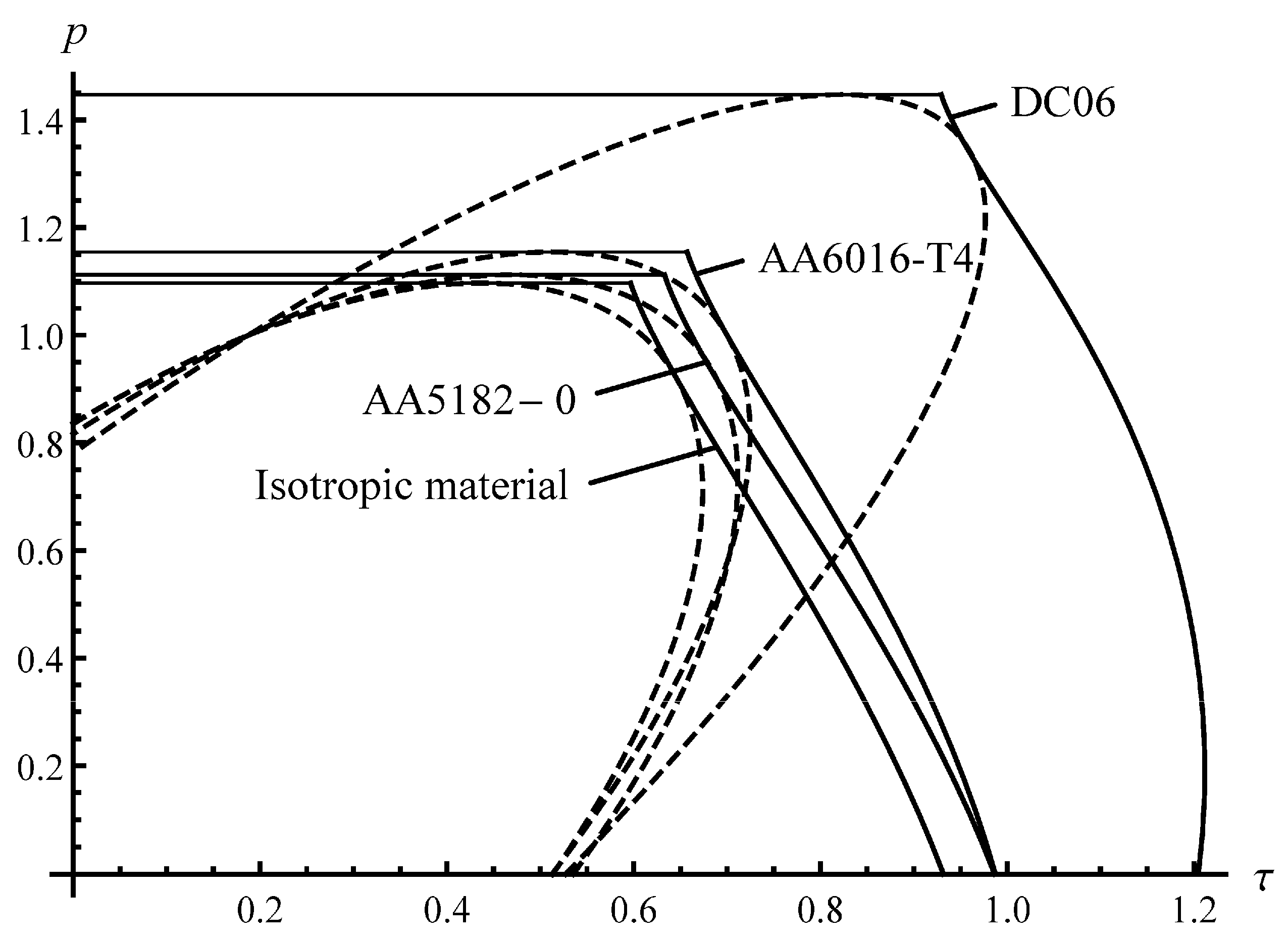
Figure 5 illustrates the elastic limit and plastic collapse curves for DC06, AA6016-T4, AA5182-0, and the isotropic material. The quantitative features of each of these curves are the same as those of the curves shown in Figure 2. The latter was already discussed in the course of constructing the solution in Section 4. Therefore, Figure 5 shows the effect of plastic anisotropy on the solution behavior.

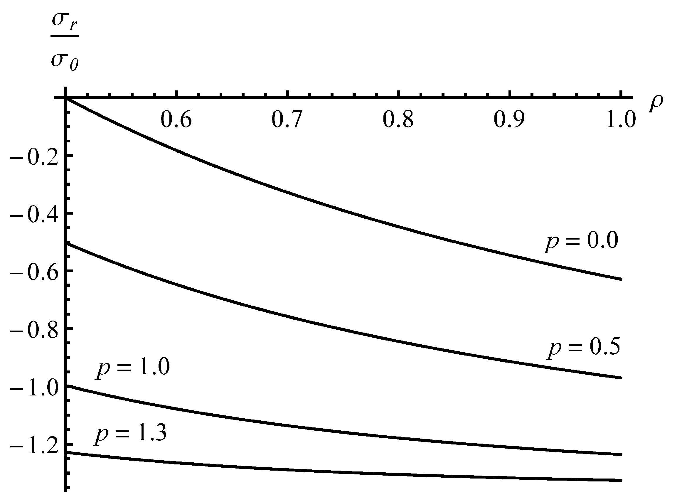
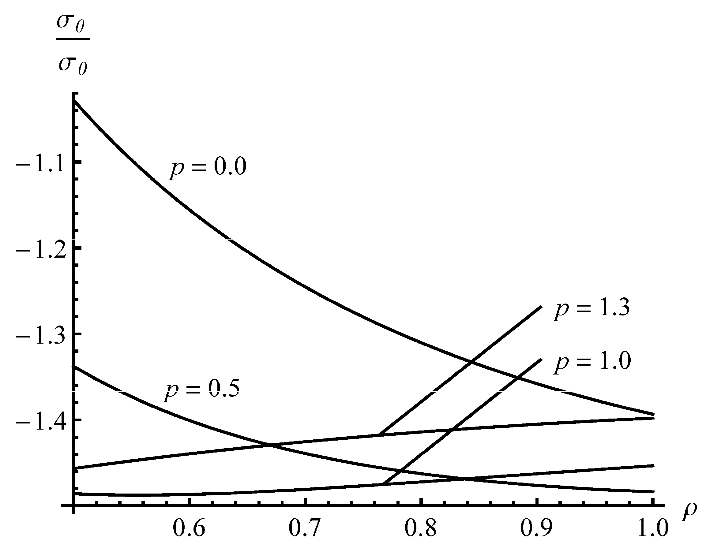
Figure 6 and Figure 7 depict the radial distribution of the radial and circumferential stresses, respectively, in a DC06 disk. The curves show the effect of the loading conditions of the stress distributions at collapse. It is worthy of note that the radial stress is a monotonically decreasing function of $\rho$ at any p. Moreover, the magnitude of this stress decreases as p decreases at any point of the disk. The qualitative behavior of the radial distribution of the circumferential stress depends on the value of p. If p is small enough, then the circumferential stress is a monotonically decreasing function of $\rho$. At intermediate values of p, the function ${\sigma }_{\theta }\left(\rho \right)$ attains a local minimum at a point of the interval $a\le \rho \le 1$. If p is large enough, then the circumferential stress is a monotonically increasing function of $\rho$.

6. Discussion

The analytic solution found revealed the following qualitative features:

• Two plastic collapse mechanisms exist. According to one of these mechanisms, the entire disk becomes plastic (curve JEH in Figure 2 and the corresponding curves in Figure 4). The other mechanism predicts the localization of plastic deformation at the inner radius of the disk (line JG in Figure 2 and the corresponding lines in Figure 5). Both mechanisms occur simultaneously at point J (Figure 2) and the corresponding points in Figure 4.
• There are two special solutions. According to one of these solutions, the entire disk becomes plastic at the initiation of plastic yielding. In this case, the curve corresponding to the elastic limit and the curve corresponding to the plastic collapse have a common point (point E in Figure 2 and the corresponding points in Figure 5). According to the other solution, the localization of plastic deformation at the inner radius of the disk occurs at the initiation of plastic yielding. In this case, the curve corresponding to the elastic limit and the curve corresponding to the plastic collapse also have a common point (point D in Figure 2 and the corresponding points in Figure 5). No plastic region of finite size exists at plastic collapse.
• Plastic yielding might initiate at the outer radius of the disk (Figure 4).
• Plastic anisotropy might have a significant effect on the plastic collapse curve (Figure 5).
• The boundary value problem is classified by three material parameters ($\eta$, ${\eta }_1$, and $\nu$), the geometric parameter a, and the loading path in the $\left(p,\hspace{0.17em}\tau \right)-$ space. Therefore, as in many other problems, for example [9], the present solution is more computationally efficient than FEM and other numerical solutions for parametric studies and preliminary design of disks. The possibility to derive this practical solution results from axial symmetry, in conjunction with the assumption of plane stress.
• The solution found can be directly used to design disks, in the manner proposed in [23].
• At p = 0, the solution found should reduce to one of the solutions given in [1]. The latter coincides with (42), if ${\psi }_a=0$. This comparison validates the solution found.

References

- Alexandrov, S. Elastic/Plastic Discs under Plane Stress Conditions; Springer Science and Business Media LLC.: New York, NY, USA, 2015. [Google Scholar]
- Kamal, S.M. Estimation of optimum rotational speed for rotational autofrettage of disks incorporating Bauschinger effect. Mech. Based Des. Struct. Mach. 2020, 1–20. [Google Scholar] [CrossRef]
- Simo, J.C.; Taylor, R.L. A return mapping algorithm for plane stress elastoplasticity. Int. J. Numer. Methods Eng. 1986, 22, 649–670. [Google Scholar] [CrossRef]
- Jetteur, P. Implicit integration algorithm for elastoplasticity in plane stress analysis. Eng. Comput. 1986, 3, 251–253. [Google Scholar] [CrossRef]
- Kleiber, M.; Kowalczyk, P. Sensitivity analysis in plane stress elasto-plasticity and elasto-viscoplasticity. Comput. Methods Appl. Mech. Eng. 1996, 137, 395–409. [Google Scholar] [CrossRef]
- Valoroso, N.; Rosati, L. Consistent derivation of the constitutive algorithm for plane stress isotropic plasticity. Part I: Theoretical formulation. Int. J. Solids Struct. 2009, 46, 74–91. [Google Scholar] [CrossRef]
- Triantafyllou, S.P.; Koumousis, V.K. An hysteretic quadrilateral plane stress element. Arch. Appl. Mech. 2012, 82, 1675–1687. [Google Scholar] [CrossRef]
- Ball, D.L. Elastic-plastic stress analysis of cold expanded fastener holes. Fatigue Fract. Eng. Mater. Struct. 1995, 18, 47–63. [Google Scholar] [CrossRef]
- Deka, S.; Mallick, A.; Behera, P.P.; Thamburaja, P. Thermal stresses in a functionally graded rotating disk: An approximate closed form solution. J. Therm. Stress. 2021, 44, 20–50. [Google Scholar] [CrossRef]
- Prime, M.B. Amplified effect of mild plastic anisotropy on residual stress and strain anisotropy. Int. J. Solids Struct. 2017, 118–119, 70–77. [Google Scholar] [CrossRef]
- Peng, X.-L.; Li, X.-F. Elastic analysis of rotating functionally graded polar orthotropic disks. Int. J. Mech. Sci. 2012, 60, 84–91. [Google Scholar] [CrossRef]
- Essa, S.; Argeso, H. Elastic analysis of variable profile and polar orthotropic FGM rotating disks for a variation function with three parameters. Acta Mech. 2017, 228, 3877–3899. [Google Scholar] [CrossRef]
- Jeong, W.; Alexandrov, S.; Lang, L. Effect of Plastic Anisotropy on the Distribution of Residual Stresses and Strains in Rotating Annular Disks. Symmetry 2018, 10, 420. [Google Scholar] [CrossRef] [Green Version]
- Yıldırım, V. Numerical/analytical solutions to the elastic response of arbitrarily functionally graded polar orthotropic rotating discs. J. Braz. Soc. Mech. Sci. Eng. 2018, 40, 320. [Google Scholar] [CrossRef]
- Aleksandrov, S.E.; Lyamina, E.A. Plastic limit state of a thin hollow disk under thermomechanical loading. J. Appl. Mech. Tech. Phys. 2012, 53, 891–898. [Google Scholar] [CrossRef]
- Alexandrov, S.; Lyamina, E.; Jeng, Y.-R. Plastic Collapse of a Thin Annular Disk Subject to Thermomechanical Loading. J. Appl. Mech. 2013, 80, 051006. [Google Scholar] [CrossRef]
- Hill, R. The Mathematical Theory of Plasticity; Clarendon Press: Oxford, UK, 1950. [Google Scholar]
- Debski, R.; Zyczkowski, M. On decohesive carrying capacity of variable-thickness annular perfectly plastic discs. Z. Angew. Math. Mech. 2002, 82, 655–669. [Google Scholar] [CrossRef]
- Alexandrov, S.; Wang, Y.-C.; Jeng, Y.-R. Elastic-Plastic Stresses and Strains in Thin Discs with Temperature-Dependent Properties Subject to Thermal Loading. J. Therm. Stress. 2014, 37, 488–505. [Google Scholar] [CrossRef]
- Alexandrova, N.; Alexandrov, S. Elastic-Plastic Stress Distribution in a Plastically Anisotropic Rotating Disk. J. Appl. Mech. 2004, 71, 427–429. [Google Scholar] [CrossRef]
- Bouvier, S.; Teodosiu, C.; Haddadi, H.; Tabacaru, V. Anisotropic work-hardening behaviour of structural steels and aluminium alloys at large strains. J. Phys. Colloq. 2003, 105, 215–222. [Google Scholar] [CrossRef]
- Wu, P.; Jain, M.; Savoie, J.; MacEwen, S.; Tuğcu, P.; Neale, K. Evaluation of anisotropic yield functions for aluminum sheets. Int. J. Plast. 2003, 19, 121–138. [Google Scholar] [CrossRef]
- Alexandrov, S.; Lyamina, E.; Jeng, Y.-R. Design of an Annular Disc Subject to Thermomechanical Loading. Math. Probl. Eng. 2012, 2012, 1–9. [Google Scholar] [CrossRef]
Figure 1.
Geometry of the boundary value problem and the boundary conditions.
Figure 2.
Generic geometric interpretation of the main features of the solution.
Figure 3.
Geometric interpretation of Equations (14) and (15): (a) generic behavior of the curves if plastic yielding initiates at the inner radius and (b) behavior of the curves for specific materials.
Figure 4.
Geometric interpretation of Equations (14) and (15) for AA3104-H19.
Figure 5.
Geometric interpretation of the collapse mechanisms for several materials.
Figure 6.
Radial distribution of the radial stress in a DC06 disk at plastic collapse for several values of p.
Figure 7.
Radial distribution of the circumferential stress in a DC06 disk at plastic collapse for several values of p.
Publisher’s Note: MDPI stays neutral with regard to jurisdictional claims in published maps and institutional affiliations. |
© 2021 by the author. Licensee MDPI, Basel, Switzerland. This article is an open access article distributed under the terms and conditions of the Creative Commons Attribution (CC BY) license (https://creativecommons.org/licenses/by/4.0/).
Share and Cite
MDPI and ACS Style
Lyamina, E. Effect of Plastic Anisotropy on the Collapse of a Hollow Disk under Thermal and Mechanical Loading. Symmetry 2021, 13, 909. https://doi.org/10.3390/sym13050909
AMA Style
Lyamina E. Effect of Plastic Anisotropy on the Collapse of a Hollow Disk under Thermal and Mechanical Loading. Symmetry. 2021; 13(5):909. https://doi.org/10.3390/sym13050909
Chicago/Turabian StyleLyamina, Elena. 2021. "Effect of Plastic Anisotropy on the Collapse of a Hollow Disk under Thermal and Mechanical Loading" Symmetry 13, no. 5: 909. https://doi.org/10.3390/sym13050909
Note that from the first issue of 2016, this journal uses article numbers instead of page numbers. See further details here.