An Accurate Limit Load Solution for an Anisotropic Highly Undermatched Tension Specimen with a Crack

Abstract

Plastic anisotropy significantly influences the behavior of structures subjected to various loading conditions. The extremum principles in the theory of rigid plastic solids are convenient and reliable tools for plastic design. The present paper combines the upper bound theorem and Hill’s quadratic yield criterion for orthotropic materials to evaluate the plastic collapse load of a highly undermatched welded tensile panel with a crack in the weld. The base material is supposed to be rigid. The shape of the crack is quite arbitrary. The orientation of the principal axes of anisotropy varies through the thickness of the weld. The upper bound solution is based on an exact solution for a layer of an anisotropic material. This feature of the upper bound solution is advantageous for increasing its accuracy. A numerical treatment is only necessary to find the solution for the uncracked specimen. This specimen has two axes of symmetry, which simplifies the solution. Simple analytic formulae transform this solution into a solution for the cracked specimens with one axis of symmetry and no symmetry. It is shown that the through-thickness distribution of anisotropic properties significantly affects the limit load.

1. Introduction

Flaw assessment procedures, such as ETM, R6, SINTAP, FITNET, BS 7910, and API 579, are widely used in engineering fracture mechanics (for example, [1,2,3,4,5]). The plastic limit load is one of the key parameters affecting the accuracy of predictions based on these procedures [6]. Compendiums of limit load solutions for structures containing cracks are available in the literature [7,8,9]. Most of these solutions are for isotropic materials. Several solutions for anisotropic materials are reviewed in [9]. These solutions and the solutions found in [10,11,12] reveal a great effect of plastic anisotropy on the limit load. An overview of the state-of-the-art application of engineering fracture mechanics to weldments are provided in [13]. This work emphasizes the inhomogeneous microstructure of the weld. The microstructure of materials, among other factors, affects the mechanical anisotropy. Some of these factors are reviewed in [14] for steels used for pipelines. Only the yield criterion affects the plastic limit load. In particular, elastic properties are immaterial for calculating the plastic limit load [15]. In the present paper, it is assumed that the yield criterion represents the current state of anisotropy, independently of the factors that have caused it. The solutions [9,10,11,12] are based on the assumption that the parameters involved in the yield criterion are constant in the weld and the base material. The review [13] strongly suggests that the distribution of anisotropic properties is not uniform within the weld. Taking into account that the effect of plastic anisotropy on various parameters resulting from elastic/plastic solutions is large [16], it is natural to expect that those non-uniform distributions of anisotropic properties may significantly affect the plastic limit load. A plane strain solution for a highly undermatched middle cracked tensile panel is proposed in [17]. This solution assumes that the weld is orthotropic and obeys Hill’s quadratic yield criterion [18]. The thickness of the weld is constant. The present paper proposes a two-fold extension of the solution [17]. Firstly, quite an arbitrary through-thickness distribution of the parameters involved in Hill’s yield criterion is assumed. Secondly, the shape of the crack is also quite arbitrary, though some restrictions apply. The method proposed in [19] is used to extend the solution for symmetric specimens to a class of the corresponding asymmetric specimens.

Other upper bound solutions for cracked specimens that account for plastic anisotropy are proposed in [10,11,12]. The solutions [11,12] are for over-matched specimens. The general method developed in the present paper is not applicable for such specimens. However, the solution [10] is for highly undermatched scarf joints. Therefore, the method developed is immediately applicable to generalize the solution [10] to non-uniform distributions of anisotropic properties and the crack of arbitrary shape.

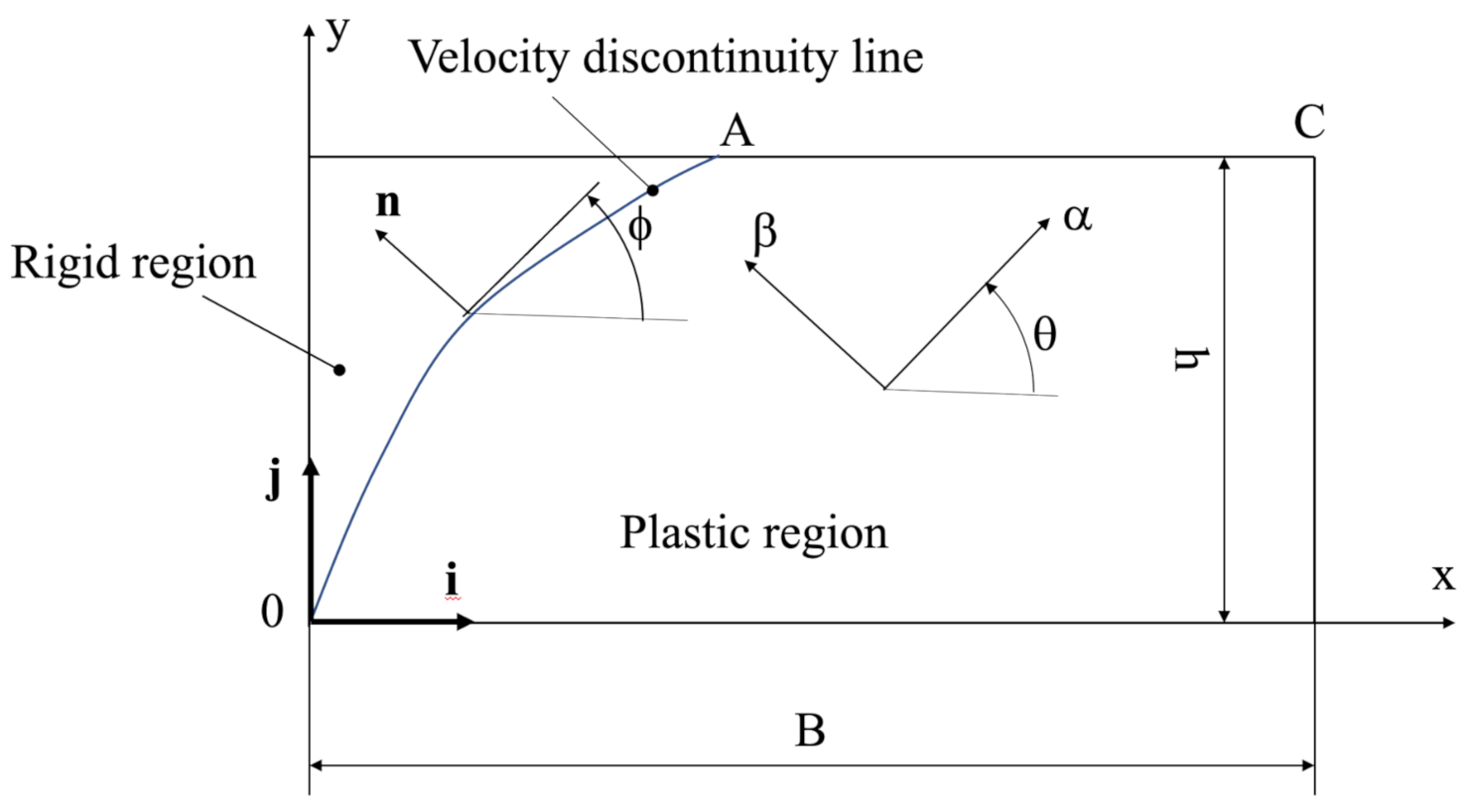
2. Statement of the Problem

A schematic diagram of the weld joint under consideration is shown in Figure 1. The width of the specimen is $2B$, and its thickness is W. The shape of a through-crack is quite arbitrary. The specific restrictions on this shape will be formulated later. The specimen is subject to tension by two forces Q. It is required to evaluate the value of Q at plastic collapse under plane strain deformation.

It is assumed that the weld is much softer than the base material. Therefore, plastic yielding occurs in the weld, whereas the base material is rigid. For this reason, the plastic properties of the base material are immaterial. The elastic properties of both the weld and base material are immaterial at plastic collapse, as follows from the theorem proven in [15]. The weld is plastically anisotropic. Let ${\sigma }_{\alpha \alpha }$, ${\sigma }_{\beta \beta }$, and ${\sigma }_{\alpha \beta }$ be the stress components referred to as the principal axes of anisotropy in planes of flow. Under plane strain conditions, Hill’s quadratic yield criterion reads as follows [18]:

$$\frac{s_{\alpha \beta }^2}{1-c}+{\sigma }_{\alpha \beta }^2=T^2.$$

(1)

Here, $s_{\alpha \beta }=\left({\sigma }_{\alpha \alpha }-{\sigma }_{\beta \beta }\right)/\phantom{\left({\sigma }_{\alpha \alpha }-{\sigma }_{\beta \beta }\right)2}2$, T is the yield stress in shear with respect to the $(\alpha ,\beta )$ axes, and c is expressed in terms of the yield stresses with respect to the principal axes of anisotropy. The expression for c is provided in [18]. For the present paper, it is sufficient to know that the following holds:

$$-\infty <c<1.$$

(2)

In the case of isotropic materials, $c=0$.

The upper bound theorem involves the plastic work rate. Let ${\xi }_{\alpha \alpha }$, ${\xi }_{\beta \beta }$, and ${\xi }_{\alpha \beta }$ be the strain rate components referred to as the principal axes of anisotropy $(\alpha ,\beta )$. The general expression for the plastic work rate per unit volume is derived in [18]. This expression reduces to the following:

$${\omega }_V=2T\sqrt{\left(1-c\right){\xi }_{\beta \beta }^2+{\xi }_{\alpha \beta }^2}$$

(3)

under plane strain deformation. It is taken into account that the material is incompressible and, therefore, ${\xi }_{\alpha \alpha }=-{\xi }_{\beta \beta }$.

We introduce a Cartesian coordinate system $(x,y)$ in the planes of flow. Let $\theta$ be the inclination of the $\alpha$-axis to the x-axis, measured counterclockwise. Then, the following holds:

$$\begin{array}{c}{\sigma }_{\alpha \alpha }=\frac{{\sigma }_{xx}+{\sigma }_{yy}}{2}+\frac{\left({\sigma }_{xx}-{\sigma }_{yy}\right)}{2}cos2\theta +{\sigma }_{xy}sin2\theta ,\hfill \\ {\sigma }_{\beta \beta }=\frac{{\sigma }_{xx}+{\sigma }_{yy}}{2}-\frac{\left({\sigma }_{xx}-{\sigma }_{yy}\right)}{2}cos2\theta -{\sigma }_{xy}sin2\theta ,\hfill \\ {\sigma }_{\alpha \beta }=-\frac{\left({\sigma }_{xx}-{\sigma }_{yy}\right)}{2}sin2\theta +{\sigma }_{xy}cos2\theta .\hfill \end{array}$$

(4)

Here, ${\sigma }_{xx}$, ${\sigma }_{yy}$ and ${\sigma }_{xy}$ are the stress components referred to as the Cartesian coordinates. Equation (4) can be rewritten as follows:

$$\begin{array}{c}{\sigma }_{xx}=\frac{{\sigma }_{\alpha \alpha }+{\sigma }_{\beta \beta }}{2}+\frac{\left({\sigma }_{\alpha \alpha }-{\sigma }_{\beta \beta }\right)}{2}cos2\theta -{\sigma }_{\alpha \beta }sin2\theta ,\hfill \\ {\sigma }_{yy}=\frac{{\sigma }_{\alpha \alpha }+{\sigma }_{\beta \beta }}{2}-\frac{\left({\sigma }_{\alpha \alpha }-{\sigma }_{\beta \beta }\right)}{2}cos2\theta +{\sigma }_{\alpha \beta }sin2\theta ,\hfill \\ {\sigma }_{xy}=\frac{\left({\sigma }_{\alpha \alpha }-{\sigma }_{\beta \beta }\right)}{2}sin2\theta +{\sigma }_{\alpha \beta }cos2\theta .\hfill \end{array}$$

(5)

Analogously,

$$\begin{array}{c}{\xi }_{\alpha \alpha }=\frac{{\xi }_{xx}+{\xi }_{yy}}{2}+\frac{\left({\xi }_{xx}-{\xi }_{yy}\right)}{2}cos2\theta +{\xi }_{xy}sin2\theta ,\hfill \\ {\xi }_{\beta \beta }=\frac{{\xi }_{xx}+{\xi }_{yy}}{2}-\frac{\left({\xi }_{xx}-{\xi }_{yy}\right)}{2}cos2\theta -{\xi }_{xy}sin2\theta ,\hfill \\ {\xi }_{\alpha \beta }=-\frac{\left({\xi }_{xx}-{\xi }_{yy}\right)}{2}sin2\theta +{\xi }_{xy}cos2\theta .\hfill \end{array}$$

(6)

Here, ${\xi }_{xx}$, ${\xi }_{yy}$, and ${\xi }_{xy}$ are the strain rate components referred to as the Cartesian coordinates.

3. Solution for the Specimen with No Crack

It will be seen later that the solution for the specimen with no crack can be immediately adopted to evaluate the limit load of the specimen with quite an arbitrary crack. A schematic diagram of the specimen considered in this section, together with the Cartesian coordinate system, is shown in Figure 2. The axes of this coordinate system coincide with the symmetry axes of the specimen.

3.1. An Exact Solution for a Layer of Anisotropic Material

Even though the upper bound theorem does not require that the equilibrium equations are satisfied, it is advantageous to choose a kinematically admissible velocity field so that the associated stress field satisfies the equilibrium equations and associated flow rule. An exact solution for the compression of an anisotropic material layer between two parallel plates is provided in [20]. Since the material is incompressible, this solution can be immediately adopted for the tension of the layer. Because of symmetry, it is sufficient to consider the solution in the first quadrant, $x\ge 0$ and $y\ge 0$. The rigid base material moves with velocity V along the y-axis. The magnitude of this velocity is immaterial.

Let $u_x$ and $u_y$ be the velocity components referred to the Cartesian coordinate system. The velocity field found in [20] is as follows:

$$\frac{u_x}{V}=-\frac{x}{h}+\frac{2}{h}\underset{h}{\overset{y}{\int }}cot2\phi d\chi +u_0,\frac{u_y}{V}=\frac{y}{h}.$$

(7)

Here, $u_0$ is constant, $\chi$ is a dummy variable of integration, and $cos2\phi$ is determined as follows:

$$cot2\phi =\frac{\partial s_{xy}}{\partial {\sigma }_{xy}}.$$

(8)

Here, $s_{xy}=\left({\sigma }_{xx}-{\sigma }_{yy}\right)/\phantom{\left({\sigma }_{xx}-{\sigma }_{yy}\right)2}2$. The pair $s_{xy}$ and ${\sigma }_{xy}$ involved in (8) should satisfy the yield criterion. The solution [20] is valid if $\phi$ is independent of x. In what follows, it is convenient to use the dimensionless quantities:

$$\zeta =\frac{y}{h},\eta =\frac{x}{B},b=\frac{B}{h}.$$

(9)

Then, Equation (7) becomes the following:

$$\frac{u_x}{V}=-\eta b+2\underset{1}{\overset{\zeta }{\int }}cot2\phi d\chi +u_0,\frac{u_y}{V}=\zeta .$$

(10)

Using (7), one can find the strain rate components as follows:

$${\xi }_{xx}=\frac{\partial u_x}{\partial x}=-\frac{V}{h},{\xi }_{yy}=\frac{\partial u_y}{\partial y}=\frac{V}{h},{\xi }_{xy}=\frac{1}{2}\left(\frac{\partial u_x}{\partial y}+\frac{\partial u_y}{\partial x}\right)=\frac{V}{h}cot2\phi .$$

(11)

Equation (1) is satisfied by the following substitution:

$$s_{\alpha \beta }=T\sqrt{1-c}cos2\gamma ,{\sigma }_{\alpha \beta }=Tsin2\gamma .$$

(12)

Here, $\gamma$ is an arbitrary function of $\zeta$. Equations (5) and (12) combine to give the following:

$$\begin{array}{c}{s}_{xy}=T\left(\sqrt{1-c}cos2\gamma cos2\theta -sin2\gamma sin2\theta \right),\hfill \\ {\sigma }_{xy}=T\left(\sqrt{1-c}cos2\gamma sin2\theta +sin2\gamma cos2\theta \right).\hfill \end{array}$$

(13)

It is seen from (8) and (13) that the condition that $\phi$ is a function only of $\zeta$ is satisfied if $\theta$ is a function only of $\zeta$. The latter is assumed in the present paper. It follows from (8) and (13) that the following holds:

$$cot2\phi =\frac{\sqrt{1-c}cos2\theta sin2\gamma +cos2\gamma sin2\theta }{\sqrt{1-c}sin2\theta sin2\gamma -cos2\gamma cos2\theta }.$$

(14)

If ${\sigma }_{xy}$ has the same value at $y=h$ and $y=-h$ (Figure 2), the solution for the shear stress given in [20] reads as follows:

$${\sigma }_{xy}=T\mu \zeta .$$

(15)

Here, $\mu$ is a constant whose value is determined by the boundary condition at $\zeta =1$. The second equation in (13) and (15) combine to provide the following:

$$\sqrt{1-c}cos2\gamma sin2\theta +sin2\gamma cos2\theta =\mu \zeta .$$

(16)

Using the trigonometric identities

$$sin2\gamma =\frac{2tan\gamma }{1+{tan}^2\gamma }\mathrm{and}cos2\gamma =\frac{1-{tan}^2\gamma }{1+{tan}^2\gamma },$$

(17)

one transforms (16) to the following:

$$\left(\mu \zeta +\sqrt{1-c}sin2\theta \right)ta{n}^2\gamma -2cos2\theta tan\gamma +\mu \zeta -\sqrt{1-c}sin2\theta =0.$$

(18)

It is a quadratic equation for $tan\gamma$. Its solution is the following:

$$tan\gamma =\frac{cos2\theta \pm \sqrt{1-c{sin}^{2}2\theta -{\mu }^2{\zeta }^2}}{\mu \zeta +\sqrt{1-c}sin2\theta }.$$

(19)

Four values of $\gamma$ are determined from this equation. The unique solution satisfies the following inequalities:

$$-\frac{\pi }{2}\le \gamma \le \frac{\pi }{2}$$

(20)

and

$$\sqrt{1-c}cos2\gamma cos2\theta -sin2\gamma sin2\theta \le 0.$$

(21)

The latter follows from the assumption that $s_{xy}\le 0$ and the first equation in (13). Substituting $\gamma$ found from (19) into (14), one finds $\phi$ as a function of $\zeta$. Then, Equation (11) supplies the strain rate components as functions of $\zeta$.

3.2. Upper Bound Solution

The general structure of the solution is illustrated in Figure 3. The velocity field (10) is kinematically admissible in the plastic region. In particular, it is seen from (11) that the incompressibility equation, ${\xi }_{xx}+{\xi }_{yy}=0$, is satisfied. It follows from (10) that $u_y=0$ at $\zeta =0$ and $u_y=V$ at $\zeta =1$. The velocity component $u_x$ does not satisfy the condition $u_x=0$ at $\eta =0$. Therefore, there must exist a rigid region that contains the y-axis (Figure 3). This region moves along the y-axis, together with the rigid base material. Therefore, its velocity is represented as follows:

$${\mathbf{U}}_{\mathbf{r}}=V\mathbf{j}$$

(22)

where $\mathbf{j}$ is one of the unit base vectors of the Cartesian coordinate system. The other unit base vector is denoted as $\mathbf{i}$. The velocity vector in the plastic region is represented as follows:

$${\mathbf{U}}_{\mathbf{p}}=u_x\mathbf{i}+u_y\mathbf{j}.$$

(23)

Here, Equation (10) supplies $u_x$ and $u_y$. Let $\varphi$ be the inclination of the tangent to velocity discontinuity line $OA$ to the x-axis, measured counterclockwise (Figure 3). Then, the unit vector normal to $OA$ is represented as follows:

$$\mathbf{n}=-\mathbf{i}sin\varphi +\mathbf{j}cos\varphi .$$

(24)

The velocity component normal to the velocity discontinuity line $OA$ must be continuous. Therefore, ${\mathbf{U}}_{\mathbf{r}}·\mathbf{n}={\mathbf{U}}_{\mathbf{p}}·\mathbf{n}$. Substituting (22), (23), and (24) into this equation and using (10), one obtains the following:

$$cos\varphi =\left[\eta b-2\underset{1}{\overset{\zeta }{\int }}cot2\phi d\chi -u_0\right]sin\varphi +\zeta cos\varphi .$$

(25)

It follows from the geometry of Figure 3 and (9) that the following holds:

$$tan\varphi =\frac{dy}{dx}=\frac{hd\zeta }{Bd\eta }=\frac{d\zeta }{bd\eta }.$$

(26)

Equations (25) and (26) combine to give the following:

$$\frac{d\eta }{d\zeta }=\frac{\eta }{1-\zeta }-\frac{2}{b\left(1-\zeta \right)}\underset{1}{\overset{\zeta }{\int }}cot2\phi d\chi -\frac{u_0}{b\left(1-\zeta \right)}.$$

(27)

It is a linear differential equation for determining the shape of the velocity discontinuity line. This line should pass through the origin of the Cartesian coordinate system. Therefore, the boundary condition to Equation (27) is $\eta =0$ for $\zeta =0$. The solution of Equation (27) satisfying this boundary condition is as follows:

$$\eta ={\eta }_{OA}\left(\zeta \right)=-\frac{2}{b\left(1-\zeta \right)}\left[\underset{0}{\overset{\zeta }{\int }}\underset{1}{\overset{\beta }{\int }}cot2\phi d\chi d\beta +\frac{\zeta u_0}{2}\right].$$

(28)

Integrating by parts, one obtains the following:

$$\underset{0}{\overset{\zeta }{\int }}\underset{1}{\overset{\beta }{\int }}cot2\phi d\chi d\beta =\zeta \underset{1}{\overset{\zeta }{\int }}cot2\phi d\chi -\underset{0}{\overset{\zeta }{\int }}\chi cot2\phi d\chi .$$

(29)

Equations (28) and (29) combine to provide the following:

$$\eta ={\eta }_{OA}\left(\zeta \right)=\frac{2}{b\left(1-\zeta \right)}\left[\underset{0}{\overset{\zeta }{\int }}\chi cot2\phi d\chi -\zeta \underset{1}{\overset{\zeta }{\int }}cot2\phi d\chi -\frac{\zeta u_0}{2}\right].$$

(30)

The velocity discontinuity line may have a common point with the line $\zeta =1$ only if the numerator in (30) vanishes at $\zeta =1$. Therefore, the following holds:

$$u_0=2\underset{0}{\overset{1}{\int }}\chi cot2\phi d\chi .$$

(31)

Substituting (31) into (30) and applying l’Hospital’s rule, one determines the value of $\eta$ at point A (Figure 3) as the following:

$${\eta }_A=\frac{2}{b}\underset{0}{\overset{1}{\int }}\chi cot2\phi d\chi .$$

(32)

The present solution is valid if the following holds:

$$0<{\eta }_A\le 1.$$

(33)

The final expression for the velocity discontinuity line follows from (30) and (31) as follows:

$$\eta ={\eta }_{OA}\left(\zeta \right)=\frac{2}{b\left(1-\zeta \right)}\left[\underset{0}{\overset{\zeta }{\int }}\chi cot2\phi d\chi -\zeta \underset{1}{\overset{\zeta }{\int }}cot2\phi d\chi -\zeta \underset{0}{\overset{1}{\int }}\chi cot2\phi d\chi \right].$$

(34)

Using (14) and (19), one can evaluate the integrals numerically. The infinitesimal length element of the velocity discontinuity line is $dL=\sqrt{{\left(dx\right)}^2+{\left(dy\right)}^2}=\sqrt{{\left(dx/\phantom{dxdy}dy\right)}^2+1}dy$. Here, the derivative $dx/dy$ is determined from (26) and (27). Then, using (9) and (30), one can represent the infinitesimal length element as follows:

$$dL={\Omega }_1\left(y\right)dy$$

(35)

where ${\Omega }_1\left(y\right)$ is a known function of y. Alternatively, using (9), one transforms the expression $dL=\sqrt{{\left(dx\right)}^2+{\left(dy\right)}^2}$ into the following:

$$dL=\sqrt{{\left(d\eta \right)}^2{B}^2+{\left(d\zeta \right)}^2{h}^2}=h\sqrt{{\left(d\eta \right)}^2{b}^2+{\left(d\zeta \right)}^2}=h\sqrt{b^2{\left(\frac{d{\eta }_{OA}}{d\zeta }\right)}^2+1}d\zeta .$$

(36)

The derivative $d{\eta }_{OA}/\phantom{d{\eta }_{OA}d\zeta }d\zeta$ is determined from (27) and (31) as follows:

$$\frac{d{\eta }_{OA}}{d\zeta }=\frac{{\eta }_{OA}\left(\zeta \right)}{1-\zeta }-\frac{2}{b\left(1-\zeta \right)}\underset{1}{\overset{\zeta }{\int }}cot2\phi d\chi -\frac{2}{b\left(1-\zeta \right)}\underset{0}{\overset{1}{\int }}\chi cot2\phi d\chi .$$

(37)

Using (34) and (37), one obtains the coefficient of $d\zeta$ in (36) as a function of $\zeta$. Then, the infinitesimal length element is represented as follows:

$$dL={\Omega }_1\left(y\right)dy={\Omega }_2\left(\zeta \right)d\zeta ,$$

(38)

where ${\Omega }_2\left(\zeta \right)$ is a known function of $\zeta$. The amount of velocity jump across the velocity discontinuity line is represented as $\left[u\right]=\left|{\mathbf{U}}_{\mathbf{r}}-{\mathbf{U}}_{\mathbf{p}}\right|$. Substituting (22) and (23) into this equation, one arrives at the following:

$$\left[u\right]=\sqrt{u_x^2+{\left(u_y-V\right)}^2}.$$

(39)

The velocity components $u_x$ and $u_y$ are understood to be calculated at the velocity discontinuity line. Therefore, Equations (10), (31) and (39) combine to give the following:

$$\frac{\left[u\right]}{V}=\sqrt{{\left[-b{\eta }_{OA}\left(\zeta \right)+2\underset{1}{\overset{\zeta }{\int }}cot2\phi d\chi +2\underset{0}{\overset{1}{\int }}\chi cot2\phi d\chi \right]}^2+{\left(\zeta -1\right)}^2}.$$

(40)

The strain rate components involved in (3) are determined from (6) and (11) as follows:

$${\xi }_{\beta \beta }=\frac{V}{h}\left(cos2\theta -cot2\phi sin2\theta \right),{\xi }_{\alpha \beta }=\frac{V}{h}\left(sin2\theta +cot2\phi cos2\theta \right).$$

(41)

Equations (3) and (41) combine to give the following:

$${\omega }_V=\frac{2TV}{h}\sqrt{\left(1-c\right){\left(cos2\theta -cot2\phi sin2\theta \right)}^2+{\left(sin2\theta +cot2\phi cos2\theta \right)}^2}.$$

(42)

It follows from the upper bound theorem and Equation (35) that the following holds:

$$QV\le 2W\left[\underset{0}{\overset{h}{\int }}\underset{B{\eta }_{OA}}{\overset{B}{\int }}{\omega }_{V}dxdy+\underset{0}{\overset{h}{\int }}\tau \left[u\right]{\Omega }_{1}dy+\underset{B{\eta }_A}{\overset{B}{\int }}{\tau }_s\left|u_x\right|dx\right].$$

(43)

The velocity component $u_x$ is understood to be calculated at $\zeta =1$. The first integral in (43) represents the plastic work rate in the plastic region, the second at the velocity discontinuity line $OA$, and the third at the velocity discontinuity line $AC$ (Figure 3). Then, $\tau$ is the actual shear stress over the velocity discontinuity line $OA$ and ${\tau }_s$ is the actual shear stress over the velocity discontinuity line $AC$.

Using (9) and (38), one can rewrite (43) as follows:

$$\frac{Q}{2TWB}\le \underset{0}{\overset{1}{\int }}\underset{{\eta }_{OA}}{\overset{1}{\int }}\frac{h{\omega }_V}{TV}d\eta d\zeta +\frac{1}{b}\underset{0}{\overset{1}{\int }}\frac{\tau }{T}\frac{\left[u\right]}{V}\frac{{\Omega }_2}{h}d\zeta +\underset{{\eta }_A}{\overset{1}{\int }}\frac{{\tau }_s}{T}\frac{\left|u_x\right|}{V}d\eta .$$

(44)

Using (42), one transforms the first integral in (44) to the following:

$$\begin{array}{c}\underset{0}{\overset{1}{\int }}\underset{{\eta }_{OA}}{\overset{1}{\int }}\frac{h{\omega }_V}{TV}d\eta d\zeta =\hfill \\ 2\underset{0}{\overset{1}{\int }}\underset{{\eta }_{OA}}{\overset{1}{\int }}\sqrt{\left(1-c\right){\left(cos2\theta -cot2\phi sin2\theta \right)}^2+{\left(sin2\theta +cot2\phi cos2\theta \right)}^2}d\eta d\zeta =\hfill \\ 2\underset{0}{\overset{1}{\int }}\sqrt{\left(1-c\right){\left(cos2\theta -cot2\phi sin2\theta \right)}^2+{\left(sin2\theta +cot2\phi cos2\theta \right)}^2}\left(1-{\eta }_{OA}\right)d\zeta .\hfill \end{array}$$

(45)

The integrand is a known function of $\zeta$. Therefore, the integral can be evaluated numerically.

Using (36) and (40), one transforms the second integral in (44) to the following:

$$\begin{array}{c}\hfill \begin{array}{c}\underset{0}{\overset{1}{\int }}\frac{\tau }{T}\frac{\left[u\right]}{V}\frac{{\Omega }_2}{h}d\zeta =\hfill \\ \underset{0}{\overset{1}{\int }}\frac{\tau }{T}\sqrt{{\left[-b{\eta }_{OA}+2\underset{1}{\overset{\zeta }{\int }}cot2\phi d\chi +2\underset{0}{\overset{1}{\int }}\chi cot2\phi d\chi \right]}^2+{\left(\zeta -1\right)}^2}\sqrt{b^2{\left(\frac{d{\eta }_{OA}}{d\zeta }\right)}^2+1}d\zeta .\hfill \end{array}\end{array}$$

(46)

Since $\tau$ is the actual shear stress over the velocity discontinuity line, its value is unknown. Therefore, the integral in (46) cannot be evaluated. In the case of isotropic materials, this difficulty is resolved by replacing $\tau$ with the shear yield stress, which is a material constant. Since $\tau$ is less or equal to the shear yield stress, this replacement cannot reduce the value of the integral in (46). Based on this argument, one concludes that the resulting right-hand side of (44) provides an upper bound on Q. However, the shear yield stress in anisotropic materials depends on the plane’s orientation over which it applies. The second equation in (13) gives the shear stress over any plane when the yield criterion is satisfied. It follows from this equation that we have the following:

$$\tau \le {\tau }_m=max\left\{T,T\sqrt{1-c}\right\}.$$

(47)

One can replace $\tau$ with ${\tau }_m$ in (44) and (46) to arrive at the following:

$$\begin{array}{c}\frac{Q_u}{2TWB}=q_u=\underset{0}{\overset{1}{\int }}\underset{{\eta }_{OA}}{\overset{1}{\int }}\frac{h{\omega }_V}{TV}d\eta d\zeta +\frac{{\tau }_m}{bT}\underset{0}{\overset{1}{\int }}\frac{\left[u\right]}{V}\frac{{\Omega }_2}{h}d\zeta +\underset{{\eta }_A}{\overset{1}{\int }}\frac{{\tau }_s}{T}\frac{\left|u_x\right|}{V}d\eta ,\hfill \\ \underset{0}{\overset{1}{\int }}\frac{{\tau }_m}{T}\frac{\left[u\right]}{V}\frac{{\Omega }_2}{h}d\zeta =\hfill \\ \frac{{\tau }_m}{T}\underset{0}{\overset{1}{\int }}\sqrt{{\left[-b{\eta }_{OA}+2\underset{1}{\overset{\zeta }{\int }}cot2\phi d\chi +2\underset{0}{\overset{1}{\int }}\chi cot2\phi d\chi \right]}^2+{\left(\zeta -1\right)}^2}\sqrt{b^2{\left(\frac{d{\eta }_{OA}}{d\zeta }\right)}^2+1}d\zeta .\hfill \end{array}$$

(48)

Here, $Q_u$ is the upper bound limit load and $q_u$ is its dimensionless representation.

The essential difference between the $OA$ and $AC$ velocity discontinuity lines is that the bi-material interface is an envelope of characteristics in the exact solution. Therefore, ${\tau }_s$ involved in the third integral in (48) is as follows [18]:

$${\tau }_s=T\sqrt{1-c{sin}^{2}2{\theta }_s}.$$

(49)

Here, ${\theta }_s$ is the value of $\theta$ at $\zeta =1$. It follows from (10), (31), and (32) that the following holds:

$$\frac{u_x}{V}=b\left({\eta }_A-\eta \right).$$

(50)

Substituting (49) and (50) into (48), one obtains the following:

$$q_u=\underset{0}{\overset{1}{\int }}\underset{{\eta }_{OA}}{\overset{1}{\int }}\frac{h{\omega }_V}{TV}d\eta d\zeta +\frac{{\tau }_m}{bT}\underset{0}{\overset{1}{\int }}\frac{\left[u\right]}{V}\frac{{\Omega }_2}{h}d\zeta +\frac{b\sqrt{1-c{sin}^{2}2{\theta }_s}{\left(1-{\eta }_A\right)}^2}{2}.$$

(51)

Using (45), (47) and the second equation in (48), one can calculate $q_u$ from (51). It follows from (15) and (49) that the following holds:

$$\mu =\sqrt{1-c{sin}^{2}2{\theta }_s}.$$

(52)

3.3. Numerical Examples

It is seen from the previous section that a numerical technique is only necessary for evaluating ordinary integrals. The Wolfram Language function NIntegrate is used for this purpose. It is assumed that $b=5$ in all calculations presented in this section. Figure 4 and Figure 5 depict the variation of the dimensionless limit load with c if $\theta$ is a constant function and a linear function of $\zeta$, respectively. The linear function is defined as $\theta ={\theta }_0\zeta$, where ${\theta }_0$ is constant. Figure 6 illustrates the effect of the through-thickness variation of $\theta$ on the dimensionless limit load. In this case, $\theta$ is represented by second-order polynomials as follows:

$$\theta =\left(\frac{\pi }{2}-\delta \right)+\delta {\zeta }^2.$$

(53)

where $\delta$ is constant. The particular case $\delta =0$ corresponds to one of the solutions shown in Figure 4. The range of $\delta$ is restricted by the condition that $sin2\theta$ is a monotonic function of $\zeta$ in the range $0\le \zeta \le 1$.

All the curves in Figure 4 and Figure 5 intersect at $c=0$ (isotropic material). The effect of $\theta$ (Figure 4) and ${\theta }_0$ (Figure 5) on the limit load increases as $\left|c\right|$ increases. The qualitative behavior of the solution is different in the ranges of $c>0$ and $c<0$. In particular, $q_u$ is an increasing function of $\left|c\right|$ for all $\theta$ (Figure 4) and all ${\theta }_0$ Figure 5) in the range $c<0$. However, it may be a decreasing or increasing function of c in the range $c>0$. Therefore, predictions of flaw assessment procedures based on the assumption of isotropic material may be non-conservative if $c>0$.

Figure 6 shows that the limit load is sensitive to the through-thickness distribution of anisotropic properties. It is particularly sensitive if $\delta$ is small. Small $\delta$-values mean that $\theta$ is close to $\pi /2$ everywhere, as follows from (53).

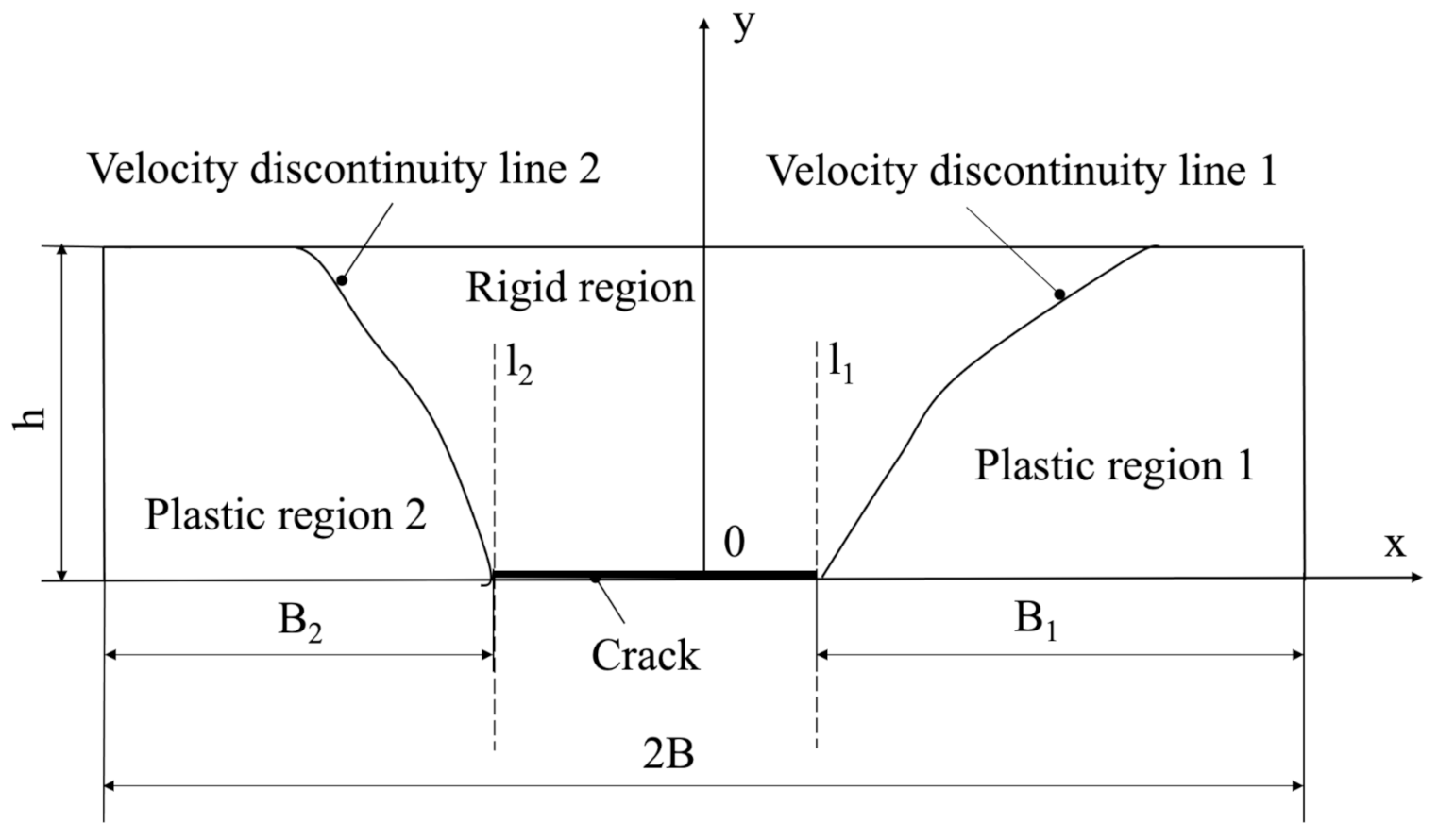
4. Solution for the Specimen with a Crack

This section demonstrates that the solution derived in Section 3 can be immediately adopted to find an upper bound limit load for a class of the specimens with a crack.

4.1. Crack on the x-Axis

As shown in Figure 2, the boundary value problem is symmetric relative to the x-axis. Therefore, it is sufficient to consider the domain $y\ge 0$. A schematic diagram of the weld and the general structure of a kinematically admissible velocity field are shown in Figure 7. It is seen from this figure that the solution from Section 3 is valid on the right to line $l_1$ if B is replaced with $B_1$. Analogously, the solution from Section 3 is valid on the left to line $l_2$ if B is replaced with $B_2$. Then, we have the following:

$$q_u=\frac{1}{2}\left(q_u^{\left(1\right)}\frac{B_1}{B}+q_u^{\left(2\right)}\frac{B_2}{B}\right).$$

(54)

Here, $q_u^{\left(1\right)}$ and $q_u^{\left(2\right)}$ are determined from (48) at $b=b_1=B_1/\phantom{B_{1}h}h$ and $b=b_2=B_2/\phantom{B_{2}h}h$, respectively. The factor 1/2 appears because (51) gives the limit load for the specimen whose width is $2B$.

Both the velocity discontinuity lines (Figure 7) should satisfy the inequality (33). Of practical importance is the inequality ${\eta }_A\le 1$. Putting ${\eta }_A=1$ in (32), one obtains the following:

$$b_m=2\underset{0}{\overset{1}{\int }}\chi cot2\phi d\chi .$$

(55)

The solution is valid if $b_1\ge b_m$ and $b_2\ge b_m$. Figure 8 depicts the variation of $b_m$ with c at several values of $\theta$, assuming that $\theta$ is constant.

4.2. Arbitrary Crack

The boundary value problem is not symmetric relative to any axis. Therefore, it is necessary to consider the entire domain occupied by the weld. A schematic diagram of the weld and the general structure of a kinematically admissible velocity field are shown in Figure 9. The kinematically admissible velocity fields on the right to $l_1$ and left to $l_2$ are taken the same as in the specimen shown in Figure 7. For the entire velocity field to be kinematically admissible, it is necessary to introduce two additional velocity discontinuity lines, $a_1{c}_1$ and $a_2{c}_2$. Then, the only restriction on the shape of the crack is that it is compatible with the motion of the two rigid regions along the y-axis in the opposite directions. The contribution of the additional velocity discontinuity lines to the right-hand side of (43) involves $\tau$. As in the case of the velocity discontinuity line $OA$ (Figure 3), one can replace $\tau$ with ${\tau }_m$ given by (47). Then, the contribution of the additional velocity discontinuity lines to the right-hand side of (43) can be represented as follows:

$${\Omega }_a=VW{\tau }_m\left(L_1+L_2\right).$$

(56)

Here, $L_1$ and $L_2$ are the lengths of lines $a_1{c}_1$ and $a_2{c}_2$, respectively. Using (47), (54), and (56), one arrives the following expression for the dimensionless limit load:

$$q_u=\frac{1}{2}\left(q_u^{\left(1\right)}\frac{B_1}{B}+q_u^{\left(2\right)}\frac{B_2}{B}\right)+\frac{1}{4}\left(\frac{{\tau }_m}{T}\right)\left(\frac{L_1}{B}+\frac{L_2}{B}\right).$$

(57)

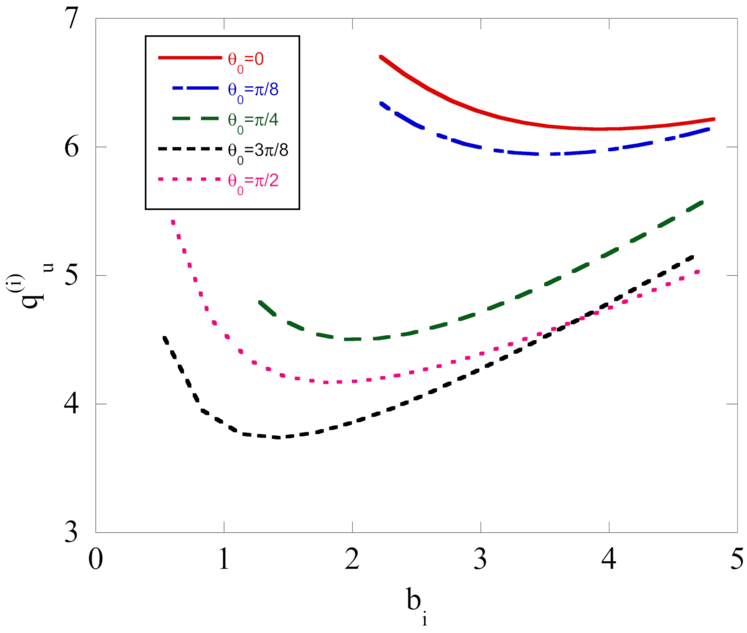
4.3. Numerical Examples

Given the mechanical properties, Equations (54) and (57) allow the limit load to be easily calculated for the specimen having any crack if the dependence of $q_u^{\left(i\right)}$ on $b_i$ is known. Here, $q_u^{\left(i\right)}=q_u^{\left(1\right)}$ and $b_i=b_1$ or $q_u^{\left(i\right)}=q_u^{\left(2\right)}$ and $b_i=b_2$. Figure 10 depicts the variation of $q_u^{\left(i\right)}$ with $b_i$ at several values of $\theta$, assuming that $\theta$ is constant. Figure 11 shows the variation of $q_u^{\left(i\right)}$ with $b_i$ at several values of ${\theta }_0$, assuming that $\theta ={\theta }_0\zeta$. The results presented in Figure 10 and Figure 11 are for $c=-1$. The left ends of the curves in Figure 10 correspond to $b_i=b_m$ (Figure 8).

The limit load for isotropic materials is an increasing function of b. An important feature of the solution illustrated in Figure 10 and Figure 11 is that the limit load considered a function of b may have a minimum if the material is anisotropic. This feature should affect the prediction of flaw assessment procedures.

5. Conclusions

A new upper bound limit load solution is proposed for a highly undermatched tension specimen containing a crack. The weld is supposed to be plastically anisotropic. The distinguishing features of this solution are (i) through-thickness variation in the plastic anisotropy, and (ii) crack of an arbitrary shape. Some restrictions of the variation in the plastic anisotropy and the shape of the crack apply, but they are not restrictive for practical applications.

An advantage of the solution is that the stress field associated with the kinematically admissible velocity field chosen satisfies the equilibrium equations. Therefore, this solution should be more accurate than other upper bound solutions of the same level of complexity.

The solution is practically analytic. A numerical technique is only required for evaluating ordinary integrals. It is particularly important because the material properties are classified by an arbitrary function rather than a set of parameters. Therefore, no parametric study is possible. However, the calculation of the limit load for any given function is fast and straightforward.

The numerical example has revealed the following interesting features of the solution: (i) predictions of flow assessment procedures based on the assumption of isotropic materials may be non-conservative for certain anisotropic materials, and (ii) the limit load is represented by a non-monotonic function of the relative thickness of the weld for certain anisotropic properties.

The solution is ready for use in conjunction with flaw assessment procedures. Such procedures are widely accepted in practical applications [1].

References

1. Zerbst, U.; Ainsworth, R.A.; Schwalbe, K.-H. Basic principles of analytical flaw assessment methods. Int. J. Press. Vessel. Pip. 2000, 77, 855–867. [Google Scholar] [CrossRef]
2. Konosu, S. Assessment procedure for multiple cracklike flaws in failure assessment diagram (FAD). ASME J. Press. Vessel Technol. 2009, 131, 041402. [Google Scholar] [CrossRef]
3. Zerbst, U.; Madia, M. Analytic flaw assessment. Eng. Fract. Mech. 2018, 187, 316–367. [Google Scholar] [CrossRef]
4. Tung, F.-Y.; Lu, Y.-J.; Wang, C.-H. Determination of the critical length of the crack-like flaws and its effect on safety. J. Loss Preven. Proc. Ind. 2021, 69, 104365. [Google Scholar] [CrossRef]
5. Fajuyigbe, A.; Brennan, F. Fitness-for-purpose assessment of cracked offshore wind turbine monopile. Marine Struct. 2021, 77, 102965. [Google Scholar] [CrossRef]
6. Zerbst, U.; Kiyak, Y.; Madia, M.; Burgold, A.; Riedel, G. Reference loads for plates with semi-elliptical surface cracks subjected to tension and bending for application within R6 type flaw assessment. Eng. Fract. Mech. 2013, 99, 132–140. [Google Scholar] [CrossRef]
7. Miller, A.G. Review of limit loads of structures containing defects. Int. J. Press. Vessel. Pip. 1988, 32, 197–327. [Google Scholar] [CrossRef]
8. Kim, Y.-J.; Schwalbe, K.-H. Compendium of yield load solutions for strength mis-matched DE(T), SE(B) and C(T) specimens. Eng. Fract. Mech. 2001, 68, 1137–1151. [Google Scholar] [CrossRef]
9. Alexandrov, S. Upper Bound Limit Load Solutions for Welded Joints with Cracks; Springer: New York, NY, USA, 2012. [Google Scholar]
10. Alexandrov, S.; Mustafa, Y. Influence of plastic anisotropy on the limit load of highly under-matched scarf joints with a crack subject to tension. Eng. Fract. Mech. 2014, 131, 616–626. [Google Scholar] [CrossRef]
11. Lyamina, E.; Kalenova, N.; Nguyen, D.K. Influence of plastic anisotropy on the limit load of an overmatched cracked tension specimen. Symmetry 2020, 12, 1079. [Google Scholar] [CrossRef]
12. Alexandrov, S.; Lyamina, E.; Pirumov, A.; Nguyen, D.K. A limit load solution for anisotropic welded cracked plates in pure bending. Symmetry 2020, 12, 1764. [Google Scholar] [CrossRef]
13. Zerbst, U. Application of fracture mechanics to welds with crack origin at the weld toe: A review. Part 1: Consequences of inhomogeneous microstructure for materials testing and failure assessment. Weld. World 2019, 63, 1715–1732. [Google Scholar] [CrossRef]
14. Joo, M.S.; Suh, D.W.; Bhadeshia, H.K.D.H. Mechanical anisotropy in steels for pipelines. ISIJ Int. 2013, 53, 1305–1314. [Google Scholar] [CrossRef] [Green Version]
15. Drucker, D.C.; Prager, W.; Greenberg, H.J. Extended limit design theorems for continuous media. Quart. Appl. Math. 1952, 9, 381–389. [Google Scholar] [CrossRef] [Green Version]
16. Prime, M.B. Amplified effect of mild plastic anisotropy on residual stress and strain anisotropy. Int. J. Solids Struct. 2017, 118, 70–77. [Google Scholar] [CrossRef]
17. Alexandrov, S.; Chung, K.-H.; Chung, K. Effect of plastic anisotropy of weld on limit load of undermatched middle cracked tension specimens. Fat. Fract. Eng. Mater. Struct. 2007, 30, 333–341. [Google Scholar] [CrossRef]
18. Hill, R. The Mathematical Theory of Plasticity; Clarendon Press: Oxford, UK, 1950. [Google Scholar]
19. Alexandrov, S. A limit load solution for a highly weld strength undermatched tensile panel with an arbitrary crack. Eng. Fract. Mech. 2010, 77, 3368–3371. [Google Scholar] [CrossRef]
20. Collins, I.F.; Meguid, S.A. On the influence of hardening and anisotropy on the plane-strain compression of thin metal strip. ASME J. Appl. Mech. 1977, 44, 271–278. [Google Scholar] [CrossRef]
Figure 1. Schematic diagram of the specimen under consideration.
Symmetry 13 01941 g001
Figure 2. Schematic diagram of the uncracked specimen and Cartesian coordinates.
Symmetry 13 01941 g002
Figure 3. General structure of the solution for the uncracked specimen.
Symmetry 13 01941 g003
Figure 4. Variation of the dimensionless limit load with c if θ is a constant.
Symmetry 13 01941 g004
Figure 5. Variation of the dimensionless limit load with c if θ is a linear function of ζ .
Symmetry 13 01941 g005
Figure 6. Effect of the through-thickness variation of θ on the dimensionless limit load.
Symmetry 13 01941 g006
Figure 7. Schematic diagram of the weld of the middle cracked specimen and the general structure of a kinematically admissible velocity field.
Symmetry 13 01941 g007
Figure 8. Geometric illustration of the solution validity condition if θ is constant.
Symmetry 13 01941 g008
Figure 9. Schematic diagram of the weld and the general structure of a kinematically admissible velocity field in the case of an arbitrary crack.
Symmetry 13 01941 g009
Figure 10. Variation of q u ( i ) with b i for several values of θ , which is a constant function.
Symmetry 13 01941 g010
Figure 11. Variation of q u ( i ) with b i for several values of θ 0 assuming that θ = θ 0 ζ .
Symmetry 13 01941 g011
Publisher’s Note: MDPI stays neutral with regard to jurisdictional claims in published maps and institutional affiliations.