Article

Hermite Cubic Spline Collocation Method for Nonlinear Fractional Differential Equations with Variable-Order

1
School of Mathematics, Lanzhou City University, Lanzhou 730070, China
2
School of Mathematics and Statistics, Lanzhou University, Lanzhou 730000, China
*
Author to whom correspondence should be addressed.
These authors contributed equally to this work.
Symmetry 2021, 13(5), 872; https://doi.org/10.3390/sym13050872
Submission received: 8 April 2021 / Revised: 9 May 2021 / Accepted: 10 May 2021 / Published: 13 May 2021
(This article belongs to the Special Issue Applied Mathematics and Fractional Calculus)

Abstract

:
In this paper, we develop a Hermite cubic spline collocation method (HCSCM) for solving variable-order nonlinear fractional differential equations, which apply C 1 -continuous nodal basis functions to an approximate problem. We also verify that the order of convergence of the HCSCM is about O ( h min { 4 α , p } ) while the interpolating function belongs to C p ( p 1 ) , where h is the mesh size and α the order of the fractional derivative. Many numerical tests are performed to confirm the effectiveness of the HCSCM for fractional differential equations, which include Helmholtz equations and the fractional Burgers equation of constant-order and variable-order with Riemann-Liouville, Caputo and Patie-Simon sense as well as two-sided cases.

1. Introduction

As a powerful tool for modeling a broad range of non-classical phenomena, fractional calculus has already gained much attention from various science and engineering fields during recent decades. For models of anomalous transport processes and diffusion, there are a lot of fractional partial differential equations proposed in publications [1,2] as well as for the modeling of frequency dependent damping behavior such as in viscoelastic, continuum and statistical mechanics, solid mechanic, economics [3,4], and so on. For modelling the energy supply-demand system, the Caputo-Fabrizio fractional derivative is applied and leads to an interesting fractional energy supply-demand equation [5]. With extensive applications of fractional calculus operators, many fractional differential equations (FDEs) are presented.
Meanwhile, there is increasing demand for a robust method to produce a high accuracy solution to FDEs. Publications on numerical methods for FDEs are largely substantial. A considerable number of them are based on finite difference, see [6,7,8,9,10,11,12,13,14,15,16,17] and the references therein. There are many works based on finite element methods, see [18,19,20,21,22,23]. Methods based on spectral/pseudo-spectral or collocation methods, even the spectral element method, can be seen in [24,25,26,27,28,29,30,31,32,33].
The main challenge of approximating FDEs is the precision deterioration caused by singularity of fractional derivatives [34]. For the spectral-type methods, which are one of the most popular numerical methods due to their high accuracy [35,36,37,38], the singularity of endpoints may damage “the spectral accuracy”. Spectral or collocation methods using fractional polynomials rather than polynomials as basis functions provide a promising way to develop an efficient algorithm for numerically solving FDEs and even fractional operator-related problems. There are theoretical and practical efforts involved in publications such as [29,39,40,41,42,43,44,45,46,47,48].
The demand of flexibility may lead researchers to pursue a multi-domain method or domain decomposition method. A multi-domain spectral collocation method (MDSCM) is suggested to numerically solve FDEs [49]. Authors make use of piecewise continuous ( C 0 ) nodal basis functions to approximate the problem. However, a piecewise continuous function may have infinite derivatives of fractional-order. Let us introduce the following result from [49]:
Lemma 1.
Let α ( 0 , 2 ) be a constant, and a , b , c R such that a < c < b . If u C 2 [ a , c ] C 2 [ c , b ] C [ a , b ] and u ( c ) and u ( c + ) exist, then
R L D a , x α u ( x ) = k = 0 1 ( x a ) k α Γ ( k + 1 α ) u ( k ) ( a ) + ( x c ) 1 α Γ ( 2 α ) [ u ( c + ) u ( c ) ] + s ( x ) ,
for any x ( c , b ) , where
s ( x ) = 1 Γ ( 3 α ) d d x a x u ( τ ) ( x τ ) 2 α d τ , if α ( 0 , 1 ) , 1 Γ ( 4 α ) d 2 d x 2 a x u ( τ ) ( x τ ) 3 α d τ , if α ( 1 , 2 ) .
Here, the R L D a , x α denotes the left Riemann-Liouville fractional derivative of α -order; we will give its definition in the following section. The above lemma shows that lim x c R L D a , x α u ( x ) = if the conditions u ( c + ) u ( c ) and α > 1 are satisfied. To overcome this drawback, C 1 -continuous nodal basis functions are needed. It is well-known that spline functions are a special class of piecewise polynomials, which provide continuous differentiable solutions over the whole spatial domain with great accuracy. One promising candidate as a C 1 -continuous nodal basis function is the Hermite cubic spline function.
Spline collocation methods are successfully applied to numerical approximation of differential equations (see [50,51,52] and references therein). However, there are a few publications devoted to the spline collocation method for FDEs. Recently, Liu et al. [53] presented an interesting result of stability and convergence of quadratic spline collocation method for time-dependent fractional diffusion equations. Majeed et al. [54] applied the cubic B-spline collocation method to solve time fractional Burgers’ and Fisher’s equations. Khalid et al. [55] presented a non-polynomial quintic spline collocation method to solve fourth-order fractional boundary value problems involving products terms. Emadifar et al. [56] explored exponential spline interpolation with multiple parameters to find solutions of fractional boundary value problem and conducted the convergence analysis for this technique.
In this paper, our aim is to develop a Hermite cubic spline collocation method (HCSCM) for solving variable-order nonlinear fractional differential equations, which makes use of C 1 -continuous nodal basis functions to approximate a problem. In particular, the collocation fractional differentiation matrix is derived for fractional derivatives in various senses including Riemann-Liouville, Caputo, Patie-Simon. The main contributions of this work are as follows:
  • A set of C 1 nodal basis functions are constructed and the corresponding collocation fractional differentiation matrix is derived for the discretization.
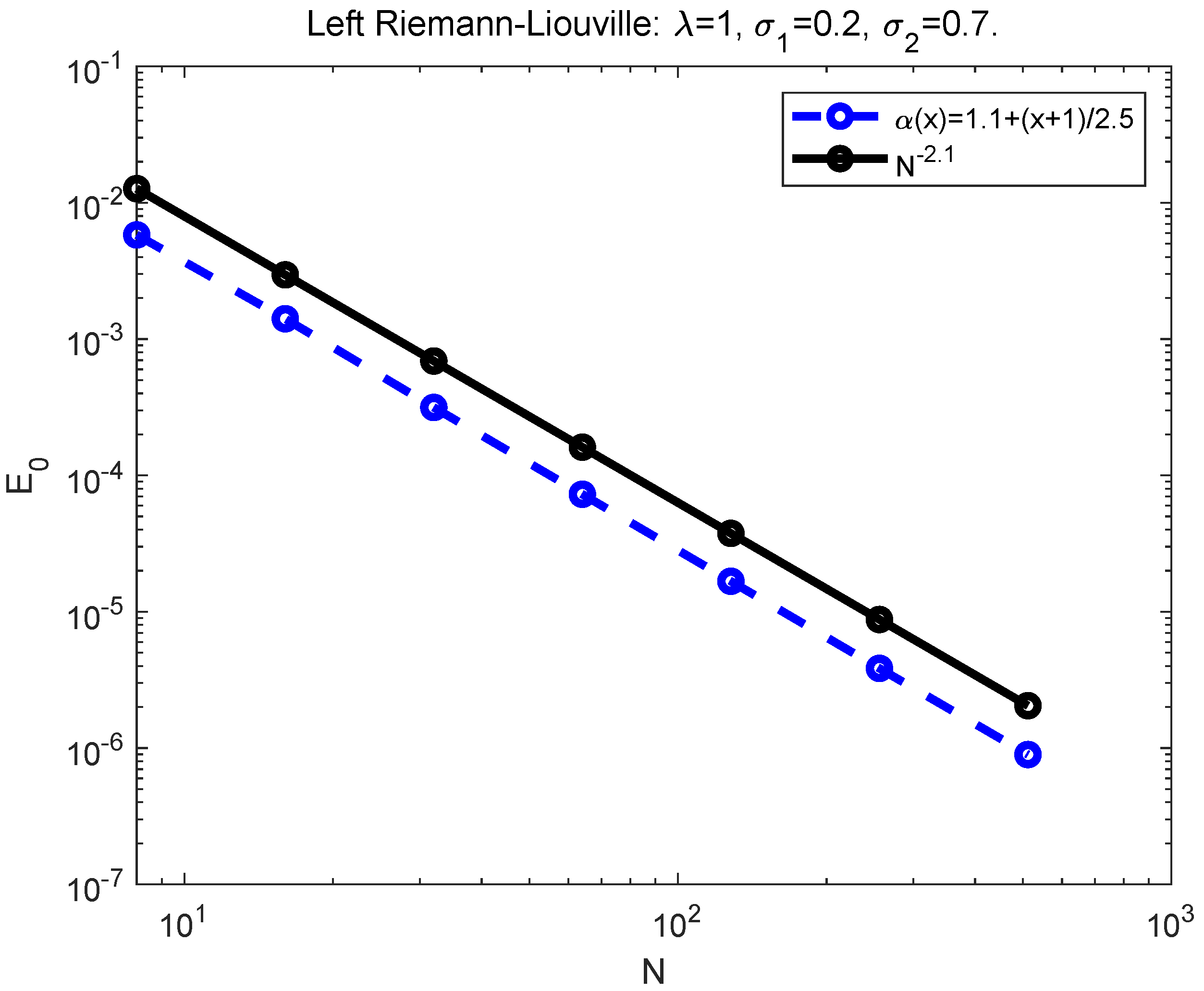
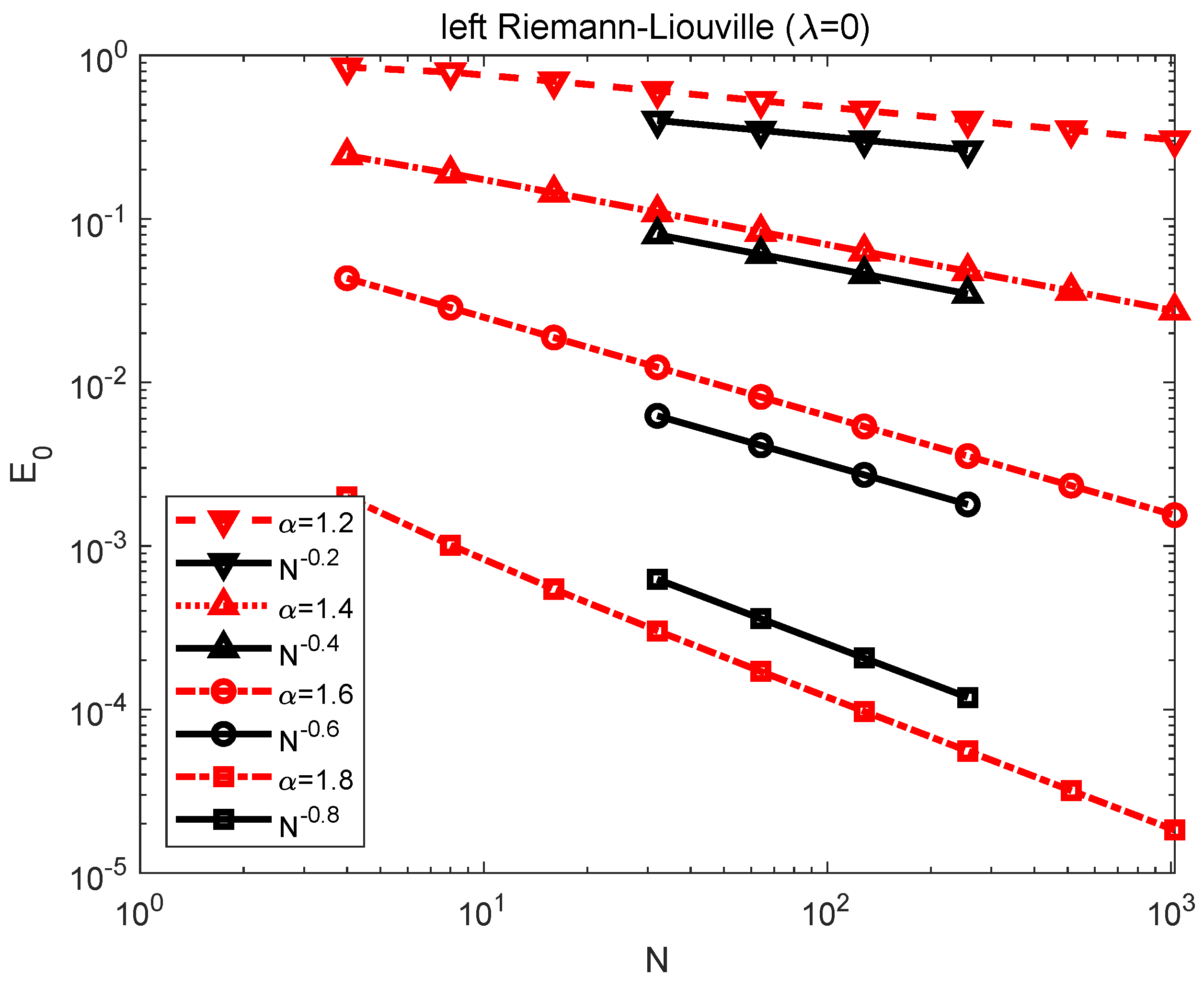
  • Making use of the Hermite cubic spline collocation method, numerical solution could be found for variable-order nonlinear fractional differential equations. The order of convergence of the HCSCM is also analysed for the left Riemann-Liouville case.
  • The effectiveness of the HCSCM is confirmed by solving fractional Helmholtz equations of constant-order and variable-order. With application the HCSCM to the fractional Burgers equation, the numerical fractional diffusion is simulated with different senses.
The paper is organized as follows: in the next Section, some definitions and properties are reviewed for later discussion. The Hermite cubic spline collocation method (HCSCM) is presented in Section 3. The key part is to set up the collocation fractional differentiation matrix. In Section 4, the order of convergence of the HCSCM approximation is analyzed for the left Riemann-Liouville case. Several numerical tests are presented in Section 5. This includes applying HCSCM to fractional Helmholtz equations and fractional Burgers equations. Finally, we conclude in Section 6.

2. Preliminaries

In this Section, some definitions of fractional calculus are reviewed for subsequent discussions. The most common-used definitions of fractional derivatives are possibly the Riemann-Liouville’s and the Caputo’s, found in various publications, such as ([57,58]). The following definitions are variable-order versions, which provide constant-order definitions when α ( x ) α is a constant in the formulas.
Definition 1.
For a function f ( x ) , x [ x L , x R ] , the left Riemann-Liouville fractional integral of order α ( x ) > 0 is defined as
x L I x α ( x ) f ( x ) : = 1 Γ ( α ( x ) ) x L x ( x s ) α ( x ) 1 f ( s ) d s ,
and the right Riemann-Liouville fractional integral of order α ( x ) > 0 is defined as
x I x R α ( x ) f ( x ) : = 1 Γ ( α ( x ) ) x x R ( s x ) α ( x ) 1 f ( s ) d s ,
where Γ ( · ) is the Euler’s gamma function.
Definition 2.
For a function f ( x ) , x [ x L , x R ] , the left Riemann-Liouville fractional derivative of order α ( x ) > 0 is defined as
R L D x L , x α ( x ) f ( x ) : = 1 Γ ( n α ( x ) ) d n d ξ n x L ξ ( ξ s ) n α ( x ) 1 f ( s ) d s ξ = x ,
and the right Riemann-Liouville fractional derivative of order α ( x ) > 0 is defined as
R L D x , x R α ( x ) f ( x ) : = ( 1 ) n Γ ( n α ( x ) ) d n d ξ n ξ x R ( s ξ ) n α ( x ) 1 f ( s ) d s ξ = x ,
where n is the positive integer such that n 1 < α ( x ) < n .
Definition 3.
For a function f ( x ) , x [ x L , x R ] , the left Caputo fractional derivative of order α ( x ) > 0 is defined as
C D x L , x α ( x ) f ( x ) : = 1 Γ ( n α ( x ) ) x L x ( x s ) n α ( x ) 1 f ( n ) ( s ) d s ,
and the right Caputo fractional derivative of order α ( x ) > 0 is defined as
C D x , x R α ( x ) f ( x ) : = ( 1 ) n Γ ( n α ( x ) ) x x R ( s x ) n α ( x ) 1 f ( n ) ( s ) d s ,
where n is the positive integer such that n 1 < α ( x ) < n .
The well-known relationship between Riemann-Liouville and the Caputo derivative is as follows:
Lemma 2.
If R L D x L , x α ( x ) f ( x ) , C D x L , x α ( x ) f ( x ) , R L D x , x R α ( x ) f ( x ) and C D x , x R α ( x ) f ( x ) exist, then
R L D x L , x α ( x ) f ( x ) = C D x L , x α ( x ) f ( x ) + k = 0 n 1 f ( k ) ( x L ) Γ ( k + 1 α ( x ) ) ( x x L ) k α ( x ) ,
and
R L D x , x R α ( x ) f ( x ) = C D x , x R α ( x ) f ( x ) + k = 0 n 1 ( 1 ) n j f ( k ) ( x R ) Γ ( k + 1 α ( x ) ) ( x R x ) k α ( x ) .
Besides the common-used definitions above, the fractional diffusion operators which limit the order 1 < α ( x ) 2 are also considered. A definition was proposed by Patie and Simon in [59] as follows.
Definition 4.
For a function f ( x ) , x [ x L , x R ] , the left Patie-Simon (or mixed Caputo) fractional derivative of order 1 < α ( x ) < 2 is defined as
P S D x L , x α ( x ) f ( x ) : = 1 Γ ( 2 α ( x ) ) d d ξ x L ξ ( ξ s ) 1 α ( x ) f ( s ) d s ξ = x ,
and the right Patie-Simon (or mixed Caputo) fractional derivative of order 1 < α ( x ) < 2 is defined as
P S D x , x R α ( x ) f ( x ) : = 1 Γ ( 2 α ( x ) ) d d ξ ξ x R ( s ξ ) 1 α ( x ) f ( s ) d s ξ = x .
From the above definitions and Lemma 2, hold the following relationships:
Lemma 3.
If 1 < α ( x ) < 2 and R L D x L , x α ( x ) f ( x ) , C D x L , x α ( x ) f ( x ) , P S D x L , x α ( x ) f ( x ) , R L D x , x R α ( x ) f ( x ) , C D x , x R α ( x ) and P S D x , x R α ( x ) f ( x ) exist, then
R L D x L , x α ( x ) f ( x ) = P S D x L , x α ( x ) f ( x ) + f ( x L ) Γ ( 1 α ( x ) ) ( x x L ) α ( x ) ,
and
R L D x , x R α ( x ) f ( x ) = P S D x , x R α ( x ) f ( x ) + f ( x R ) Γ ( 1 α ( x ) ) ( x R x ) α ( x ) ,
and
P S D x L , x α ( x ) f ( x ) = C D x L , x α ( x ) f ( x ) + f ( x L ) Γ ( 2 α ( x ) ) ( x x L ) 1 α ( x ) ,
and
P S D x , x R α ( x ) f ( x ) = C D x , x R α ( x ) f ( x ) + f ( x R ) Γ ( 2 α ( x ) ) ( x R x ) 1 α ( x ) .
Proof. 
Since
x L ξ ( ξ s ) 1 α ( x ) f ( s ) d s = ( ξ x L ) 2 α ( x ) 2 α ( x ) f ( x L ) + 1 2 α ( x ) x L ξ ( ξ s ) 2 α ( x ) f ( s ) d s .
Then note that 1 < α ( x ) < 2 ,
d 2 d ξ 2 x L ξ ( ξ s ) 1 α ( x ) f ( s ) d s = ( 1 α ( x ) ) ( ξ x L ) α ( x ) f ( x L ) + d d ξ x L ξ ( ξ s ) 1 α ( x ) f ( s ) d s ] .
The equality (11) is obtained by dividing factor Γ ( 2 α ( x ) ) . Other results can be derived by a similar argument. □
There exist the following well-known properties:
Lemma 4.
Let m be an integer number, the following properties hold for x [ x L , x R ] and Riemann-Liouville fractional calculus
x L I x α ( x ) ( x x L ) m = m ! Γ m + α ( x ) + 1 ( x x L ) m + α ( x ) , x I x R α ( x ) ( x R x ) m = m ! Γ m + α ( x ) + 1 ( x R x ) m + α ( x ) , R L D x L , x α ( x ) ( x x L ) m = m ! Γ m α ( x ) + 1 ( x x L ) m α ( x ) , R L D x , x R α ( x ) ( x R x ) m = m ! Γ m α ( x ) + 1 ( x R x ) m α ( x ) ,
and for the Caputo fractional derivative,
C D x L , x α ( x ) ( x x L ) m = m ! Γ m α ( x ) + 1 ( x x L ) m α ( x ) , i f m > α ( x ) , 0 , i f m < α ( x ) , C D x , x R α ( x ) ( x R x ) m = m ! Γ m α ( x ) + 1 ( x R x ) m α ( x ) , i f m > α ( x ) , 0 , i f m < α ( x ) ,
and for the Patie-Simon fractional derivative of 1 < α ( x ) < 2 ,
P S D x L , x α ( x ) ( x x L ) m = m ! Γ m α ( x ) + 1 ( x x L ) m α ( x ) , i f m > 0 , 0 , i f m = 0 , P S D x , x R α ( x ) ( x R x ) m = m ! Γ m α ( x ) + 1 ( x R x ) m α ( x ) , i f m > 0 , 0 , i f m = 0 .
The following operators with top-tilde are useful in HCSCM for x > x R ,
x L I ˜ x R α ( x ) f ( x ) : = 1 Γ ( α ( x ) ) x L x R ( x s ) α ( x ) 1 f ( s ) d s ,
and for x < x L ,
x L I ˜ x R α ( x ) f ( x ) : = 1 Γ ( α ( x ) ) x L x R ( s x ) α ( x ) 1 f ( s ) d s ,
and for x > x R ,
R L D ˜ x L , x R α ( x ) f ( x ) : = 1 Γ ( n α ( x ) ) d n d ξ n x L x R ( ξ s ) n α ( x ) 1 f ( s ) d s ξ = x ,
and for x < x L ,
R L D ˜ x L , x R α ( x ) f ( x ) : = ( 1 ) n Γ ( n α ( x ) ) d n d ξ n x L x R ( s ξ ) n α ( x ) 1 f ( s ) d s ξ = x .
Operators C D ˜ x L , x R α ( x ) , C D ˜ x L , x R α ( x ) , P S D ˜ x L , x R α ( x ) , P S D ˜ x L , x R α ( x ) are defined similarly.
Lemma 5.
Let x L < x c < x R and x ( x c , x R ] , then
x L I x α ( x ) f ( x ) = x L I ˜ x c α ( x ) f ( x ) + x c I x α ( x ) f ( x ) , R L D x L , x α ( x ) f ( x ) = R L D ˜ x L , x c α ( x ) f ( x ) + R L D x c , x α ( x ) f ( x ) , C D x L , x α ( x ) f ( x ) = C D ˜ x L , x c α ( x ) f ( x ) + C D x c , x α ( x ) f ( x ) , P S D x L , x α ( x ) f ( x ) = P S D ˜ x L , x c α ( x ) f ( x ) + P S D x c , x α ( x ) f ( x ) ,
and when x [ x L , x c ) , we have
x I x R α ( x ) f ( x ) = x I x c α ( x ) f ( x ) + x c I ˜ x R α ( x ) f ( x ) , R L D x , x R α ( x ) f ( x ) = R L D x , x c α ( x ) f ( x ) + R L D ˜ x c , x R α ( x ) f ( x ) , C D x , x R α ( x ) f ( x ) = C D x , x c α ( x ) f ( x ) + C D ˜ x c , x R α ( x ) f ( x ) , P S D x , x R α ( x ) f ( x ) = P S D x , x c α ( x ) f ( x ) + P S D ˜ x c , x R α ( x ) f ( x ) .
Proof. 
Since
x L x ( x s ) α ( x ) 1 f ( s ) d s = x L x c ( x s ) α ( x ) 1 f ( s ) d s + x c x ( x s ) α ( x ) 1 d s ,
Then the first equality in (22) is obtained by dividing factor Γ ( α ( x ) ) and the definitions (1) and (18). Other results can be derived by a similar argument. □
If D α ( x ) and D α ( x ) represent all left-sided and right-sided definitions of the above-mentioned, respectively, then the two-sided fractional derivative can be written as
D r α ( x ) : = r D α ( x ) + ( 1 r ) D α ( x ) , 0 r 1 .

3. Hermite Cubic Spline Collocation Method (HCSCM)

In the Section, the HCSCM is presented. The key role of HCSCM is the collocation fractional differentiation matrix.

3.1. Fractional Differentiation Matrix (FDM) for HCSCM

Let Λ : = ( x L , x R ) , the first step is to divide the interval Λ into N elements, that is,
x L = x 0 < x 1 < < x N = x R .
Denote I i = [ x i 1 , x i ] , i = 1 , 2 , , N the i th element and h i = x i x i 1 the length of I i . Let P N I be the collection of all algebraic polynomials defined on interval I with degree at most N. The piecewise Hermite cubic polynomial space is
V N = { v C 1 ( Λ ) : v | I i P 3 I i , i = 1 , 2 , , N } .
which is defined by the following set of nodal basis functions. It contains 2 N + 2 functions as follows. The first two functions as
φ 0 ( x ) = 1 + 2 x x 0 h 1 1 x x 0 h 1 2 , if x I 1 , 0 , otherwise ,
and
ϕ 0 ( x ) = x x 0 h 1 1 x x 0 h 1 2 h 1 , if x I 1 , 0 , otherwise .
For i = 1 , 2 , , N 1 ,
φ i ( x ) = 3 2 x x i 1 h i x x i 1 h i 2 , if x I i , 1 + 2 x x i h i + 1 1 x x i h i + 1 2 , if x I i + 1 , 0 , otherwise ,
and
ϕ i ( x ) = 1 x x i 1 h i x x i 1 h i 2 h i , if x I i , x x i h i + 1 1 x x i h i + 1 2 h i + 1 , if x I i + 1 , 0 , otherwise .
and the last two functions as
φ N ( x ) = 3 2 x x N 1 h N x x N 1 h N 2 , if x I N , 0 , otherwise ,
and
ϕ N ( x ) = 1 x x N 1 h N x x N 1 h N 2 h N , if x I N , 0 , otherwise .
Therefore,
V N = span { φ i , ϕ i , i = 0 , 1 , , N } .
If u N V N , then can be expanded as
u N ( x ) = i = 0 N u N ( x i ) φ i ( x ) + u N ( x i ) ϕ i ( x ) .
In each element I i , x i , 1 c , x i , 2 c I i are the collocation points, where
x i , 1 c = x i 1 + σ i , 1 h i , x i , 2 c = x i 1 + σ i , 2 h i , i = 1 , 2 , , N ,
and 0 σ i , 1 < σ i , 2 1 . In fact, a choice of this points is the Gauss-type quadrature nodes, σ i , 1 = ( 1 σ i , 2 ) = 3 3 , which is named by orthogonal spline collocation. However, the stable collocation points may not be symmetric in the view of [60,61].
As a collocation approximation to the α ( x ) th-order differential operators defined in Section 2, we denote by D α the collocation fractional differentiation matrix, which satisfies
( D α u N ) l = D α ( x i j c ) u N ( x i j c ) , j = 1 , 2 ; i = 1 , 2 , , N .
The structure of the collocation fractional differentiation matrix (FDM) may differ with the ordering of the collocation points and the unknowns. In natural ordering l = 2 ( i 1 ) + j , we have
u = [ u 0 , u 1 , u 1 , , u N 1 , u N 1 , u N ] T , x c = [ x 11 c , x 12 c , x 21 c , x 22 c , , x N 1 c , x N 2 c ] T .
and D α with Dirichlet boundary conditions is
D α = D ϕ 0 ( x 11 c ) D φ 1 ( x 11 c ) D ϕ 1 ( x 11 c ) D ϕ N ( x 11 c ) D ϕ 0 ( x 12 c ) D φ 1 ( x 12 c ) D ϕ 1 ( x 12 c ) D ϕ N ( x 12 c ) D ϕ 0 ( x N 1 c ) D φ 1 ( x N 1 c ) D ϕ 1 ( x N 1 c ) D ϕ N ( x N 1 c ) D ϕ 0 ( x N 2 c ) D φ 1 ( x N 2 c ) D ϕ 1 ( x N 2 c ) D ϕ N ( x N 2 c ) ,
here D = D α ( x i j c ) is one of the fractional differential operators defined in Section 2. Typically, the matrix D is block-triangular for left and right fractional operators.
Remark 1.
According to the Lemma 2, Lemma 3 and the special nodal basis functions, the collocation FDM D α of the Riemann-Liouville operators is equal to the corresponding FDM of the Patie-Simon operators. For the Caputo operators, the corresponding FDM is different only from the first or last column.

3.2. Computing the Entries of FDM

For ease of computing, operations are shifted from an arbitrary interval [ a , b ] to the reference interval [ 1 , 1 ] . Let the linear transformation
x = h 2 y + 1 + a , or y = 2 h x a 1 , h : = b a
shift functions f ( x ) , α ( x ) defined on the interval [ a , b ] to f ^ ( y ) , α ^ ( y ) on the reference interval [ 1 , 1 ] . Then we have the following relations:
a I x α ( x ) f ( x ) = h 2 α ^ ( y ) 1 I y α ^ ( y ) f ^ ( y ) , x I b α ( x ) f ( x ) = h 2 α ^ ( y ) y I 1 α ^ ( y ) f ^ ( y ) , D α ( x ) f ( x ) = 2 h α ^ ( y ) D α ^ ( y ) f ^ ( y ) ,
here D α ( x ) be one of the seven: R L D a , x α ( x ) ,   R L D x , b α ( x ) , C D a , x α ( x ) ,   C D x , b α ( x ) , P S D a , x α ( x ) , P S D x , b α ( x ) , D r α ( x ) .
For the tilde operators, the following relations also hold:
a I ˜ b α ( x ) f ( x ) = h 2 α ^ ( y ) 1 I ˜ 1 α ^ ( y ) f ^ ( y ) , a I ˜ b α ( x ) f ( x ) = h 2 α ^ ( y ) 1 I ˜ 1 α ^ ( y ) f ^ ( y ) , D ˜ α ( x ) f ( x ) = 2 h α ^ ( y ) D ˜ α ^ ( y ) f ^ ( y ) ,
here D ˜ α ( x ) can be one of the six: R L D ˜ a , b α ( x ) , R L D ˜ a , b α ( x ) , C D ˜ a , b α ( x ) , C D ˜ a , b α ( x ) , P S D ˜ a , b α ( x ) , P S D ˜ a , b α ( x ) .
The nodal basis functions presented in Section 3, are the so-called shape functions after being transferred by (28), that is,
ξ 1 ( y ) : = ( 2 + y ) 1 y + 1 2 2 , ξ 2 ( y ) : = y + 1 2 1 y + 1 2 2 , ( except   factor h i ) , ξ 3 ( y ) : = 2 y y + 1 2 2 , ξ 4 ( y ) : = 1 y + 1 2 y + 1 2 2 , ( except   factor h i ) ,
and y [ 1 , 1 ] . The Hermite Spline collocation method will perform all the operators mentioned above on the shape functions (31).

4. Order of Convergence of the Approximation with HCSCM

In this Section, the order of convergence of the approximation with HCSCM is analysed. Typically, the left Riemann-Liouville fractional derivative is considered. For convenience of analysis, denote D α = R L D x L , x α ( x ) and let h i = x i x i 1 = h , σ i , 1 = σ 1 , σ i , 2 = σ 2 , i = 1 , 2 , , N . Then x i = x 0 + i h , i = 0 , 1 , , N and the collocation points
x i , 1 c = x 0 + ( i 1 + σ 1 ) h , x i , 2 c = x 0 + ( i 1 + σ 2 ) h , i = 1 , 2 , , N .
Let Π N : C 1 ( Λ ) V N be the piecewise Hermite cubic interpolation operator, determined uniquely by
Π N f ( x i ) = f ( x i ) , d d x ( Π N f ) ( x i ) = f ( x i ) , i = 0 , 1 , , N ,
for every f C 1 ( Λ ) .
For a function u ( x ) C ( Λ ) , the maximum norm is defined by
u = max x Λ | u ( x ) | .
The following results are related to the interpolation errors [62].
Lemma 6.
Let u ( x ) C 4 ( Λ ) . Then
d j d x j u Π N u C h 4 j u ( 4 ) , 0 j 3 ,
where C is a constant number which do not dependent on N.
If u ( x ) C p ( Λ ) ( p 1 ) , the interpolation error holds (see [63]):
d j d x j u Π N u C h s j u ( s ) , 0 j p .
where s = min { p , 4 } .
In the following, the error bound is presented for D α ( Π N u u ) with constant-order α ( 1 , 2 ) . Let τ ( x ) = Π N u u , we have
D α τ ( x ) = 1 Γ ( 2 α ) d 2 d x 2 x L x τ ( s ) ( x s ) α 1 d s .
Assume that x [ x j 1 , x j ] for some j, then the above integration can be split as
x L x τ ( s ) ( x s ) α 1 d s = i = 1 j 1 x i 1 x i τ ( s ) ( x s ) α 1 d s + x j 1 x τ ( s ) ( x s ) α 1 d s .
Let x ¯ i = ( x i 1 + x i ) / 2 , i = 1 , 2 , , N . Under the assumption of u ( x ) C 4 ( Λ ) , from Taylor’s theorem we have
d 2 d x 2 x i 1 x i τ ( s ) ( x s ) α 1 d s = k = 0 3 τ ( k ) ( x ¯ i ) k ! d 2 d x 2 x i 1 x i ( s x ¯ i ) k ( x s ) α 1 d s + 1 24 d 2 d x 2 x i 1 x i u ( 4 ) ( ζ i ) ( s x ¯ i ) 4 ( x s ) α 1 d s = : k = 0 3 J k ( x ) + J 4 ( x ) ,
where ζ i ( x i 1 , x i ) . Now from the Mean Value Theorem for integrals for k = 0 , 1 , 2 , 3
J k ( x ) = τ ( k ) ( x ¯ i ) k ! ( ζ ^ i , k x ¯ i ) k ( α 1 ) [ ( x x i ) α ( x x i 1 ) α ] ,
and
J 4 ( x ) = u ( 4 ) ( ζ ˜ i ) ( ζ ^ i , 4 x ¯ i ) 4 24 ( α 1 ) ( x x i ) α ( x x i 1 ) α ,
where ζ ˜ i , ζ ^ i , k ( x i 1 , x i ) . For the second integral in (34), we have
d 2 d x 2 x j 1 x τ ( s ) ( x s ) α 1 d s = τ ( x ¯ j ) ( 1 α ) ( x x j 1 ) α + τ ( x ¯ j ) h 2 ( 1 α ) ( x x j 1 ) α + ( x x j 1 ) 1 α + τ ( x ¯ j ) 2 [ h 2 4 ( 1 α ) ( x x j 1 ) α h ( x x j 1 ) 1 α + 2 2 α ( x x j 1 ) 2 α ] + τ ( x ¯ j ) 6 [ h 3 8 ( 1 α ) ( x x j 1 ) α + 3 h 2 4 ( x x j 1 ) 1 α + 3 h 2 α ( x x j 1 ) 2 α + 6 ( 2 α ) ( 3 α ) ( x x j 1 ) 3 α ] + u ( 4 ) ( ζ ˜ j ) ( ζ ^ j x ¯ j ) 4 24 ( 1 α ) ( x x j 1 ) α = : J ( x ) .
Let σ h = x x j 1 . Note that σ ( 0 , 1 ) , it is easy to know that
σ α > σ α ( σ + 1 ) α > ( σ + 1 ) α ( σ + 2 ) α >
Hence, by Lemma 6, for k = 0 , 1 , 2 , 3 and every i < j we have
| J k ( x ) | | τ ( k ) ( x ¯ i ) | k ! h k α ( α 1 ) σ α ( σ + 1 ) α C h 4 α u ( 4 ) ,
and
| J 4 ( x ) | | u ( k ) ( ζ ˜ i ) | 4 ! h 4 α ( α 1 ) σ α ( σ + 1 ) α C h 4 α u ( 4 ) ,
and
| J ( x ) | τ ( x ¯ j ) h α ( 1 α ) σ α + τ ( x ¯ j ) h 1 α ( 1 α ) 2 σ α + σ 1 α + τ ( x ¯ j ) h 2 α 1 α 8 σ α 1 2 σ 1 α + 1 2 α σ 2 α + τ ( x ¯ j ) h 3 α α 1 48 σ α + σ 1 α 8 + σ 2 α 2 ( 2 α ) + σ 3 α ( 2 α ) ( 3 α ) + ( ζ j ^ x ¯ j ) 4 h α u ( 4 ) ( ζ ˜ j ) 24 ( 1 α ) σ α C h 4 α u ( 4 ) .
Now collecting the inequalities (40)–(42) gives the following result for the case of p = 4 .
Theorem 1.
If u ( x ) C p ( Λ ) and p 1 an integer number, then it holds the error estimate:
D α ( Π N u u ) C h min { p , 4 α } u ( p ) ,
where C independent on N.
Proof of Theorem 1.
When p = 1 , the Taylor’s theorem gives
d 2 d x 2 x i 1 x i τ ( s ) ( x s ) α 1 d x = [ τ ( x ¯ i ) + τ ( ζ ˜ i ) ( ζ ^ i x ¯ i ) ] ( α 1 ) [ ( x x i ) α ( x x i 1 ) α ] ,
and
d 2 d x 2 x j 1 x τ ( s ) ( x s ) α 1 d x = [ τ ( x ¯ j ) + τ ( ζ ˜ j ) ( ζ ^ j x ¯ j ) ] ( α 1 ) [ ( x x j 1 ) α ] .
So, by (33), the estimate (43) follows. For the cases p = 2 and p = 3 , the estimate (43) can be obtained by a similar argument. □
Remark 2.
For a real number p ( 0 , 1 ) , the numerical tests show that the estimate (43) also holds.

5. Applications to Fractional Differential Equations

In this Section, some numerical examples are presented to demonstrate the efficiency of our approximation method. The following three types of meshes are used in numerical tests:
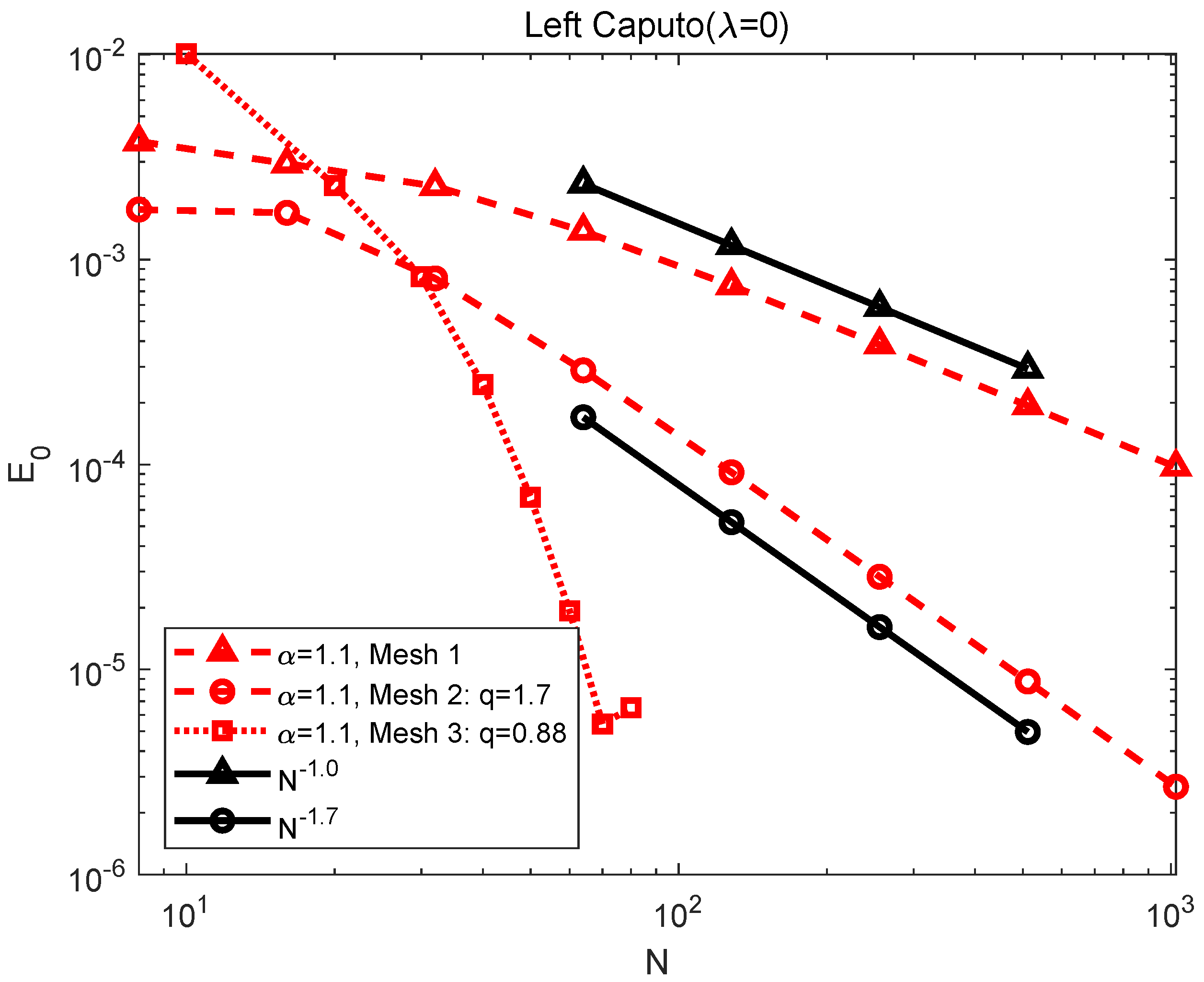
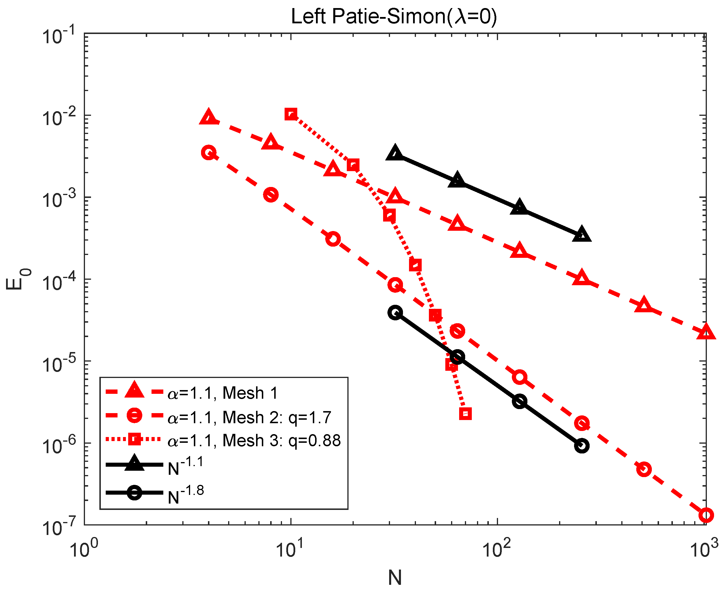
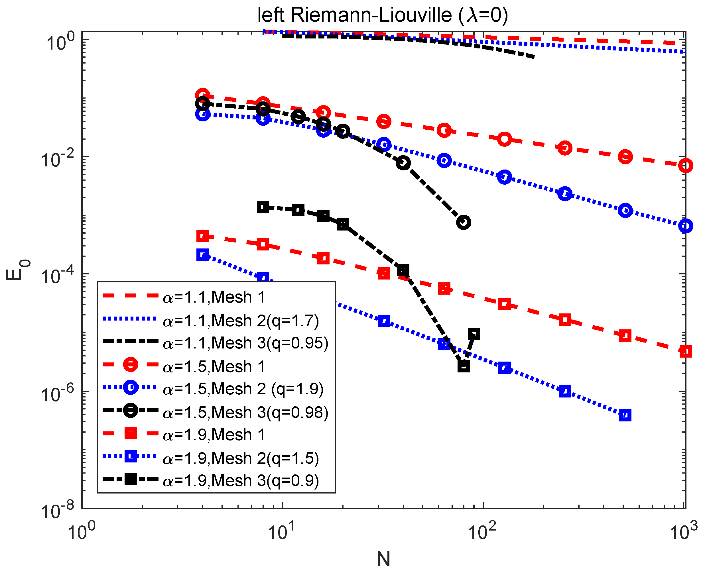
  • Uniform mesh (Mesh 1):
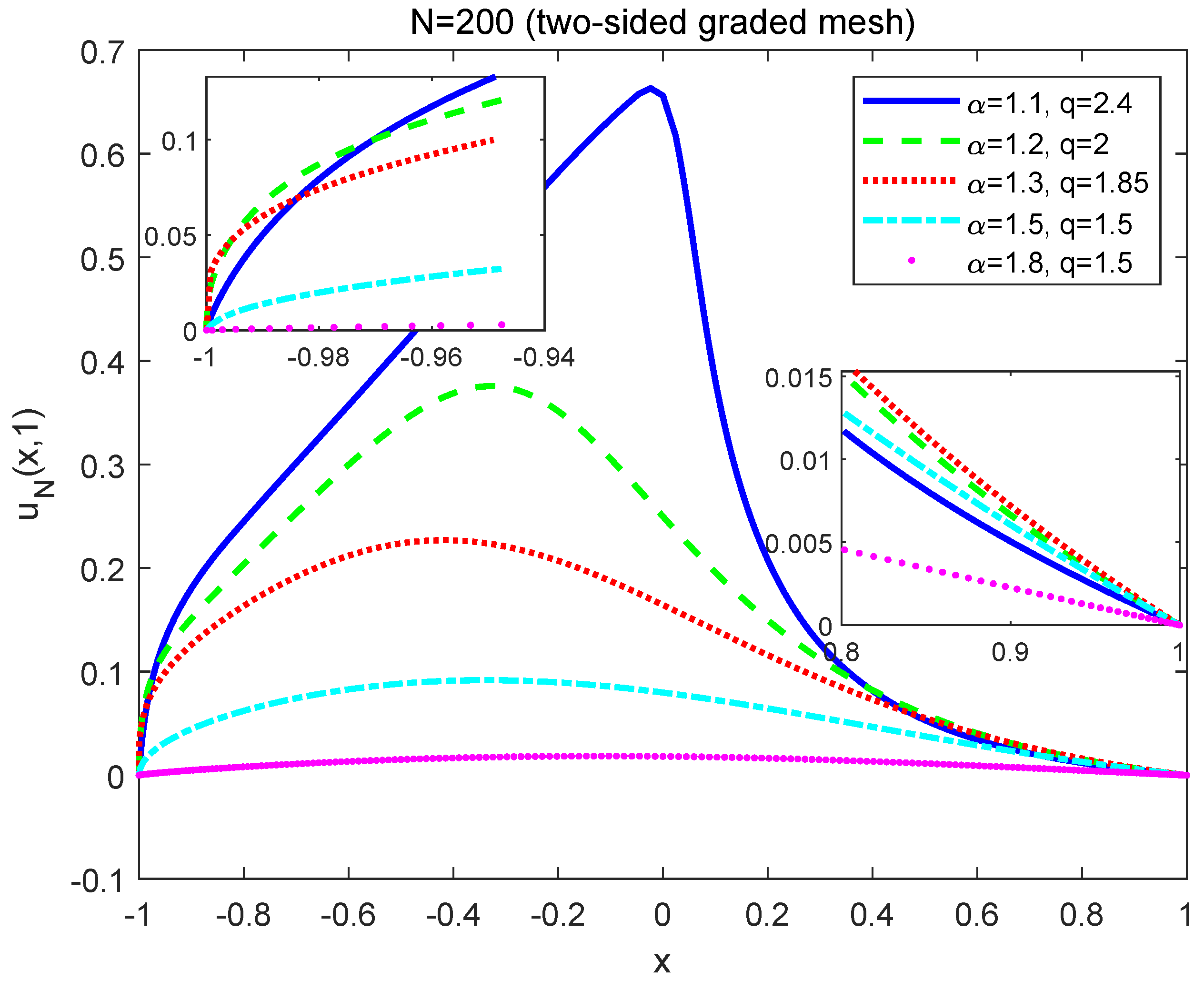
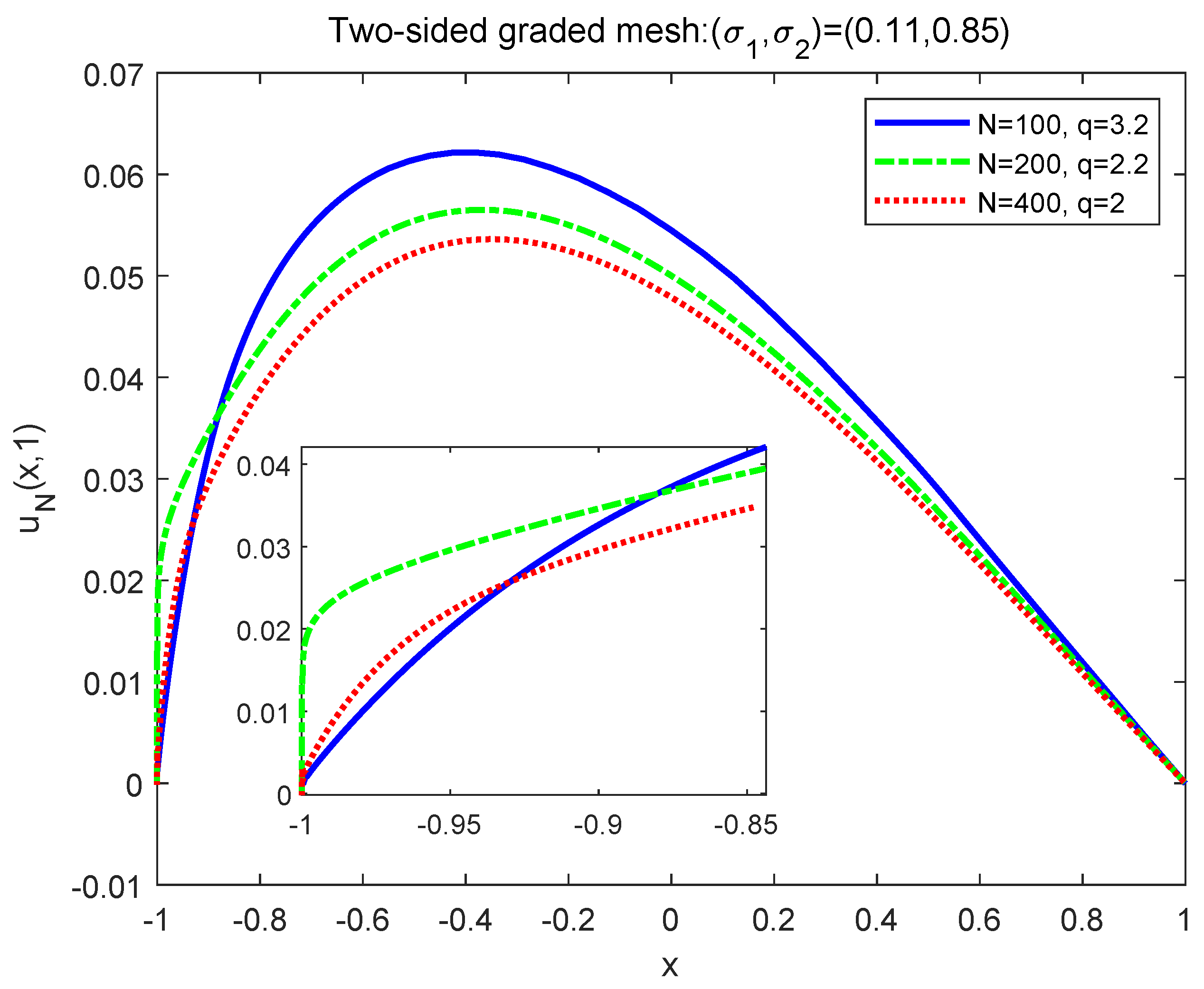
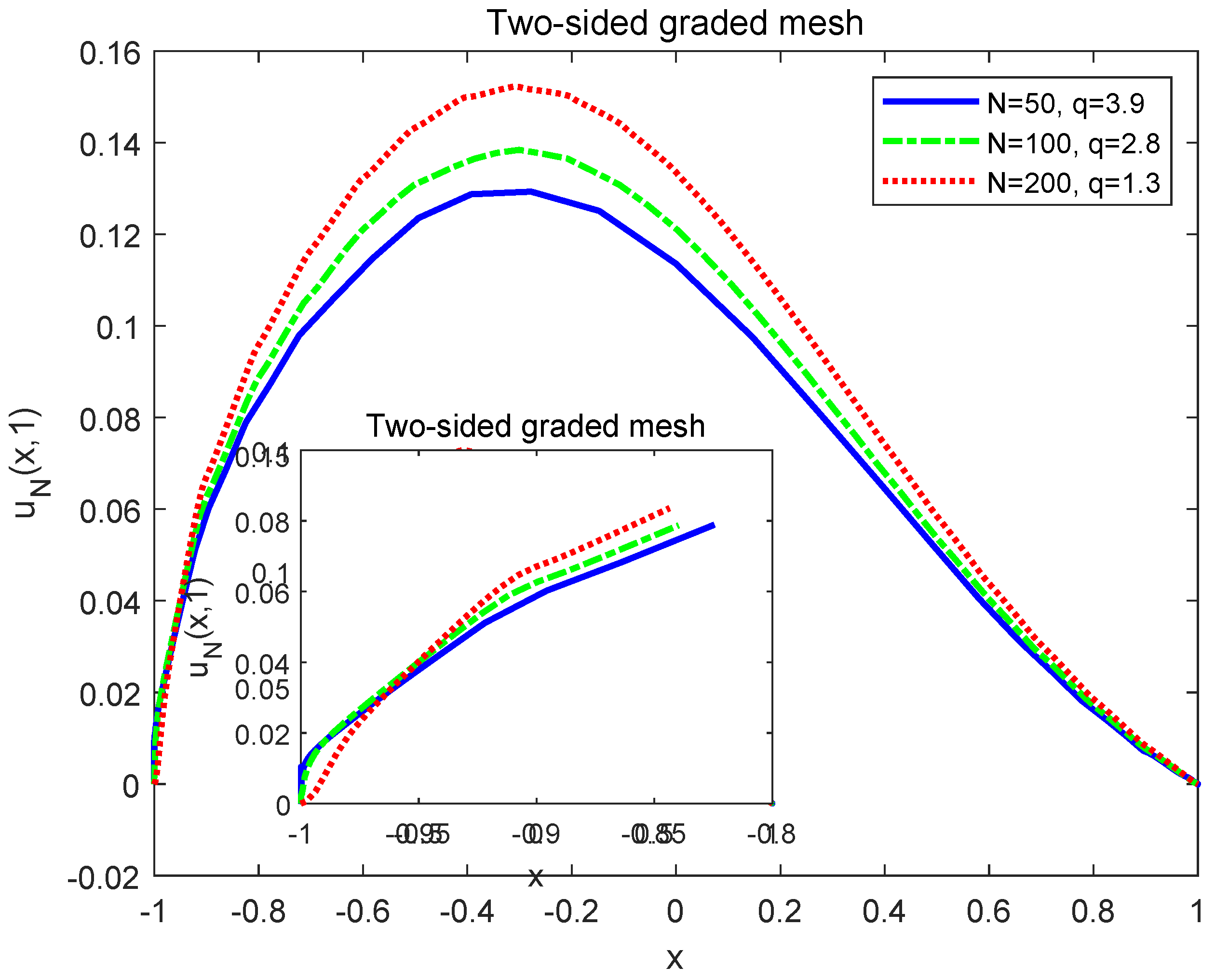
    x j = x L + ( x R x L ) j N , j = 0 , 1 , , N .
  • Graded mesh (Mesh 2):
    x j = x L + ( x R x L ) j N q , q > 1 , j = 0 , 1 , , N .
    Note: For the two-sided operator, two-sided graded mesh will be used with an even number N:
    x j = x L + ( x R x L ) 2 j N h q 1 , j = 0 , 1 , , N h x j = x R ( x R x L ) 2 N j N h q 2 , j = N h + 1 , N h + 2 , N ,
    where N h = N 2 and when q = q 1 = q 2 , the two-sided mesh is symmetric.
  • Geometric mesh (Mesh 3):
    x 0 = x L , x j = x L + ( x R x L ) q N j , 0 < q < 1 , j = 1 , 2 , , N .

5.1. Fractional Helmholtz Equations

To measure the accuracy of the HCSCM when the exact solution is known, we define the errors by
E 0 = max x { x 1 , x 2 , , x N 1 } { | u N ( x ) u ( x ) | } ,
where u N ( x ) and u ( x ) are numerical and exact solution respectively. Let Λ : = ( x L , x R ) and 1 < α ( x ) < 2 . In this subsection we apply the HCSCM to the following variable-order fractional Helmholtz equation with homogeneous boundary conditions
λ 2 u ( x ) D α ( x ) u ( x ) = f ( x ) , x Λ , u ( x L ) = u ( x R ) = 0 .
The HCSCM for (44) is to find u N V N , such that
λ 2 u N ( x ) D α ( x ) u N ( x ) = f ( x ) , x x c , u N ( x L ) = u N ( x R ) = 0 .
The above equation leads to the following linear system:
λ 2 M D α u = f
where M = [ ϕ 0 ( x c ) , φ 1 ( x c ) , ϕ 1 ( x c ) , , φ N 1 ( x c ) , ϕ N 1 ( x c ) , ϕ N ( x c ) ] is the collocation matrix, x c and u as in (26), f = f ( x c ) and D α is the fractional differentiation matrix with respect to the fractional operator D α ( x ) as in (27).
Example 1.
Our first test of HCSCM is to consider the problem (44) with exact solution u ( x ) = sin ( π x ) at [ x L , x R ] = [ 1 , 1 ] .
The right-hand side function f ( x ) = λ 2 u ( x ) D α ( x ) u ( x ) in which the fractional derivative term is approximated by when D α ( x ) = R L D 1 , x α ( x )
R L D 1 , x α ( x ) sin ( π x ) = k = 0 L ( 1 ) k + 1 π 2 k + 1 ( x + 1 ) 2 k + 1 α ( x ) Γ ( 2 k + 2 α ( x ) ) ,
and when D α ( x ) = R L D x , 1 α ( x )
R L D x , 1 α ( x ) sin ( π x ) = k = 0 L ( 1 ) k π 2 k + 1 ( 1 x ) 2 k + 1 α ( x ) Γ ( 2 k + 2 α ( x ) ) ,
with L = 50 , respectively.
For α ( x ) , we consider the following two cases:
  • The constant-order α = 1.1 , 1.2 , 1.4 , 1.5 , 1.6 , 1.8 , 1.9 .
  • The variable-order α ( x ) = 1.1 + x + 1 2.5 .
The aim of this example is to test the accuracy of the proposed method for the smooth solution. In this example, the uniform mesh is used. The error E 0 and the orders of convergence are listed in Table 1. It is shown that the order of convergence of the approximation is 4 α .
The error E 0 and CPU time for α = 1.4 are listed in Table 2. Similar results can be obtained for other cases. All the computations are performed by Matlab R2020a on pc with AMD PRO A10-8770 R7, 10 COMPUTE CORES 4C+6G 3.50GHz. The Matlab route inv is used to solve the linear system (46) in our numerical tests. Other faster solver such as LU decomposition, iteration-type methods and so forth might be used to improve the efficiency.
The error E 0 is given in Figure 1 and Figure 2. In Figure 1, it is clearly shown that the orders of convergence of approximation is about 4 α which confirms the estimate in Theorem 1. In Figure 2, the orders of convergence of approximation is about
4 max 1 x 1 α ( x )
for the variable-order case.
Example 2.
Our second test of HCSCM is to consider the problem (44) with an exact solution that has low regularity.
When we take u ( x ) = ( 1 x ) ( 1 + x ) α ( x ) with x L = 1 , x R = 1 , the right-hand functions are same for left Riemann-Liouville, left Caputo and left Patie-Simon cases, that is,
f ( x ) = λ 2 u ( x ) 2 Γ ( 1 + α ( x ) ) + Γ ( 2 + α ( x ) ) ( 1 + x ) .
In fact, here we have u ( x ) C α ( Λ ) .
The error E 0 and the orders of convergence are listed in Table 3. It is shown that the order of convergence of the approximation is α .
The error E 0 for uniform mesh and for α = 1.1 , 1.5 , 1.9 are shown in Figure 3. It is clear that the order of convergence of E 0 is α .
The error E 0 for α = 1.2 with three types of mesh are shown in Figure 4. It is shown that the uniform mesh achieves an α order of convergence of E 0 and the graded mesh improves significantly the order of convergence. We can also observe that the geometric mesh might achieve “higher accuracy” (see the dotted line with squares Figure 3), although the precisions are damaged for large N. The errors E 0 for the Caputo case and Patie-Simon case are plotted in Figure 5 and Figure 6.
If we take u ( x ) = ( 1 x ) ( 1 + x ) α ( x ) 1 , it means that u ( x ) C α 1 ( Λ ) , which has very low regularity with x L = 1 , x R = 1 and then the right-hand function
f ( x ) = λ 2 u ( x ) + Γ ( 1 + α ( x ) )
for left Riemann-Liouville and left Patie-Simon cases (but not for left Caputo case).
The error E 0 and the orders of convergence are listed in Table 4. It is shown that the order of convergence of the approximation is α 1 .
The errors E 0 are plotted in Figure 7, Figure 8, Figure 9 and Figure 10. Compared the Figure 4 with the Figure 7, we can find that the orders of convergence of E 0 are dropped to α 1 for the exact solution that belongs to C α 1 ( Λ ) , which agree with the results in Theorem 1. It is also observed that the orders of convergence of E 0 are improved by making use of the graded mesh and the geometric mesh similarly.
The HCSCM is comparable to the MDSCM [49] since both of them are applied piecewise polynomial to approximation problems. The numerical errors are compared by using the HCSCM and the MDSCM. The maximum errors with the degree of freedom are plotted for the constant-order α = 1.1 , 1.5 and 1.9 and for the variable-order α ( x ) = 1.1 + ( x + 1 ) / 2.5 in Figure 9 and Figure 10. The black lines are for the MDSCM with fixed N = 3 and the penalty parameter τ = 100,000. By the choice of N = 3 of the MDSCM, the degree of piecewise polynomial in the HCSCM is the same as ones in the MDSCM. Both the uniform meshes are applied for two methods. It is shown that the accuracy of the HCSCM is better than those of the MDSCM [49] with h-refinement but the orders of convergence are almost same.

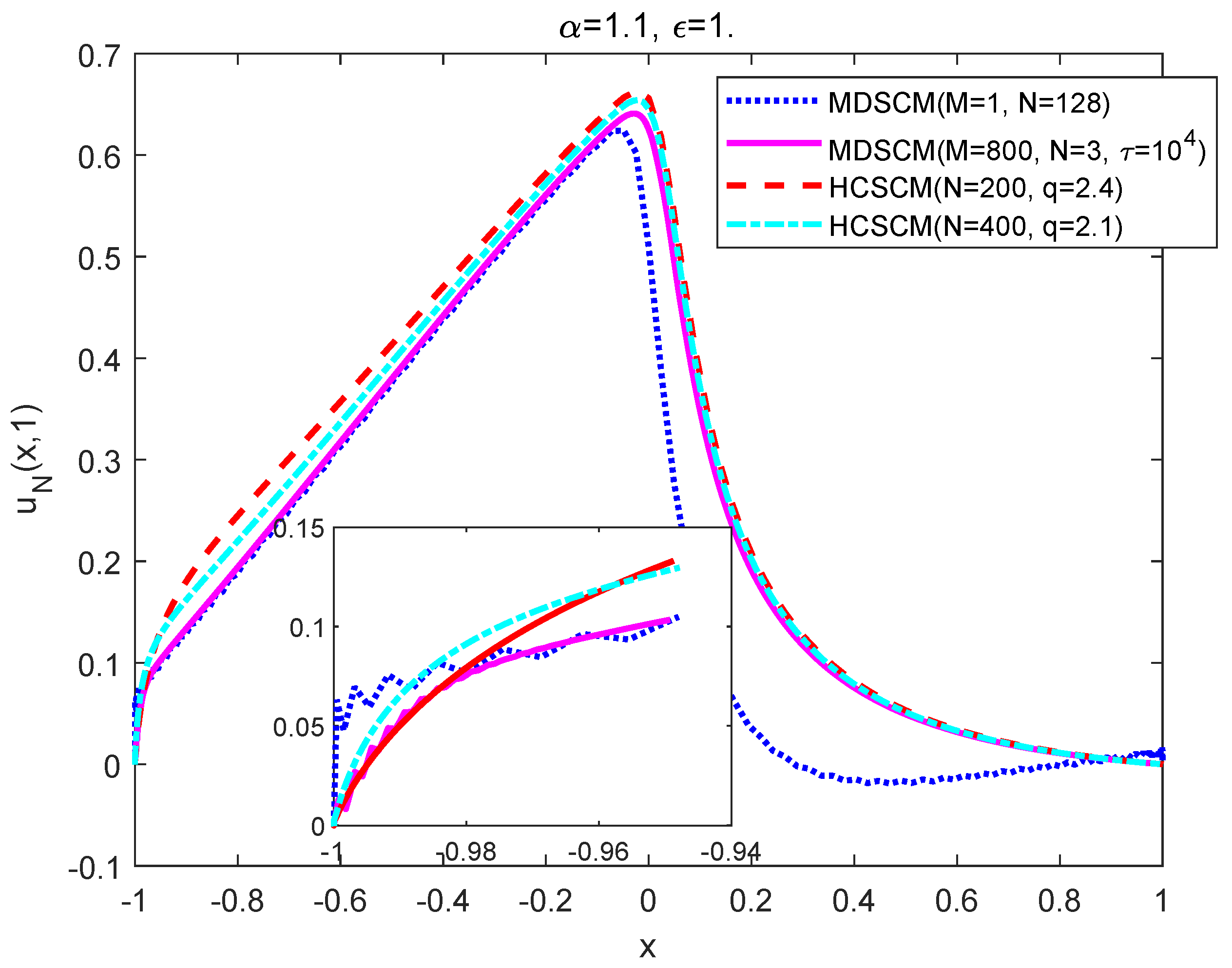
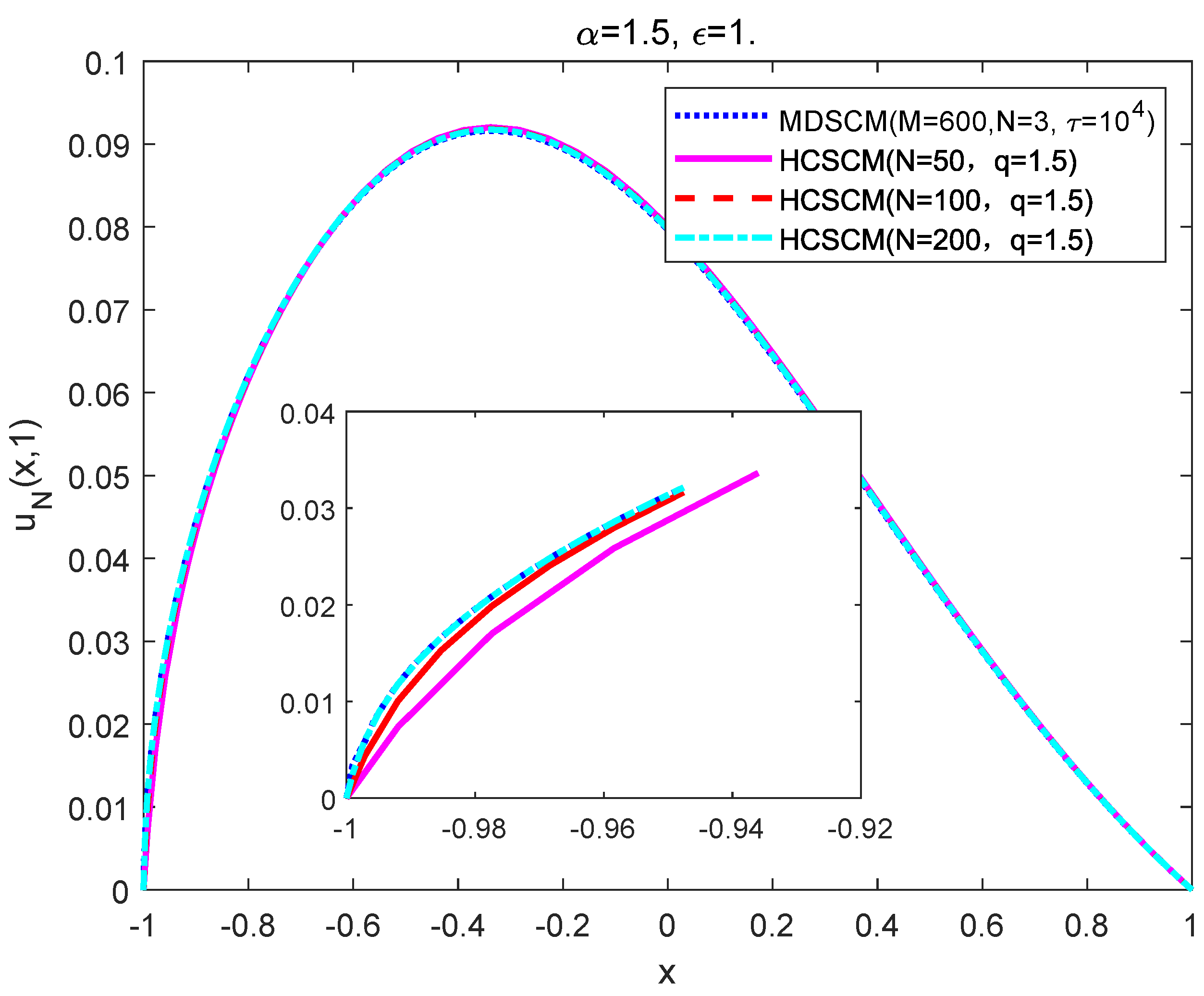
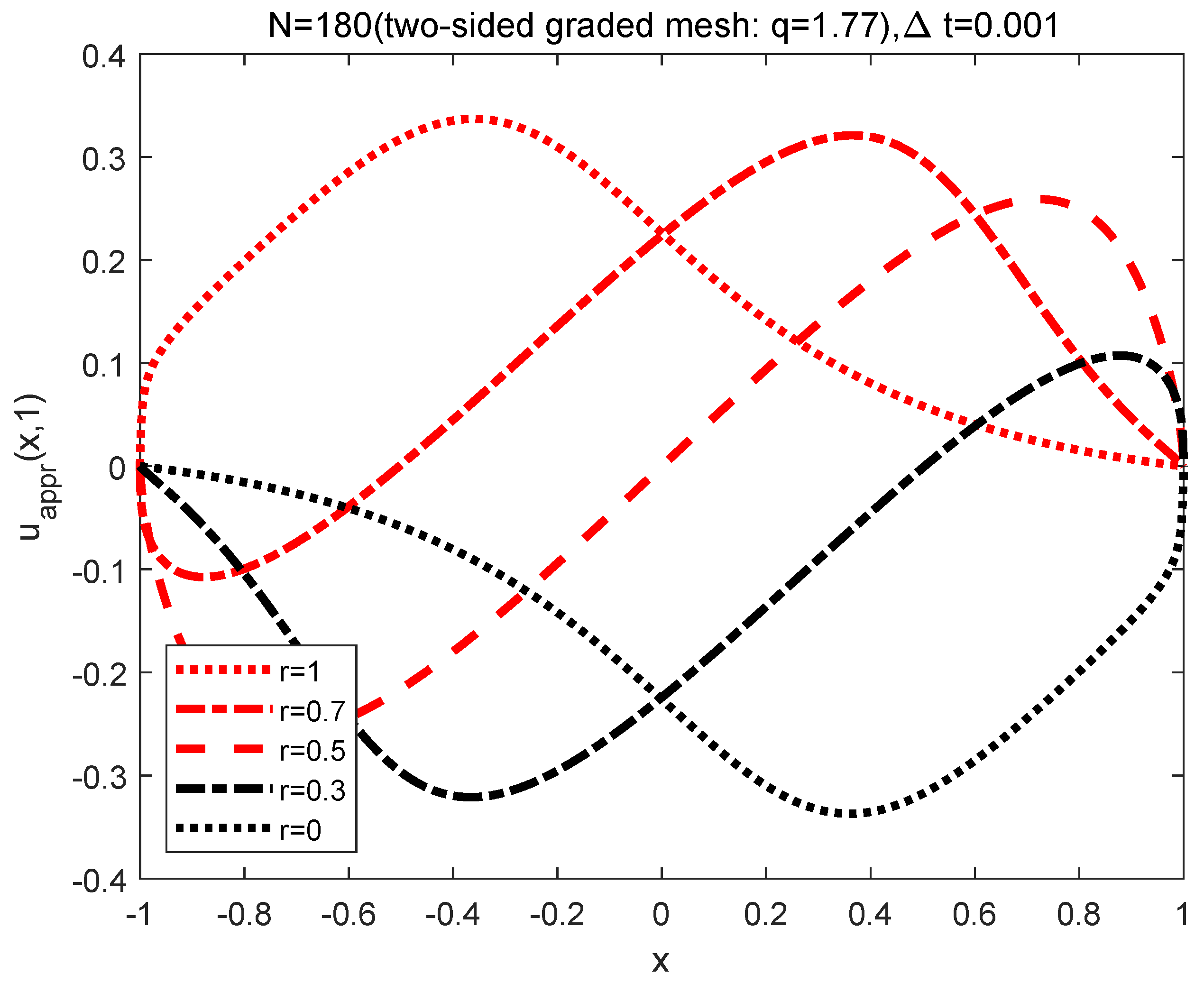
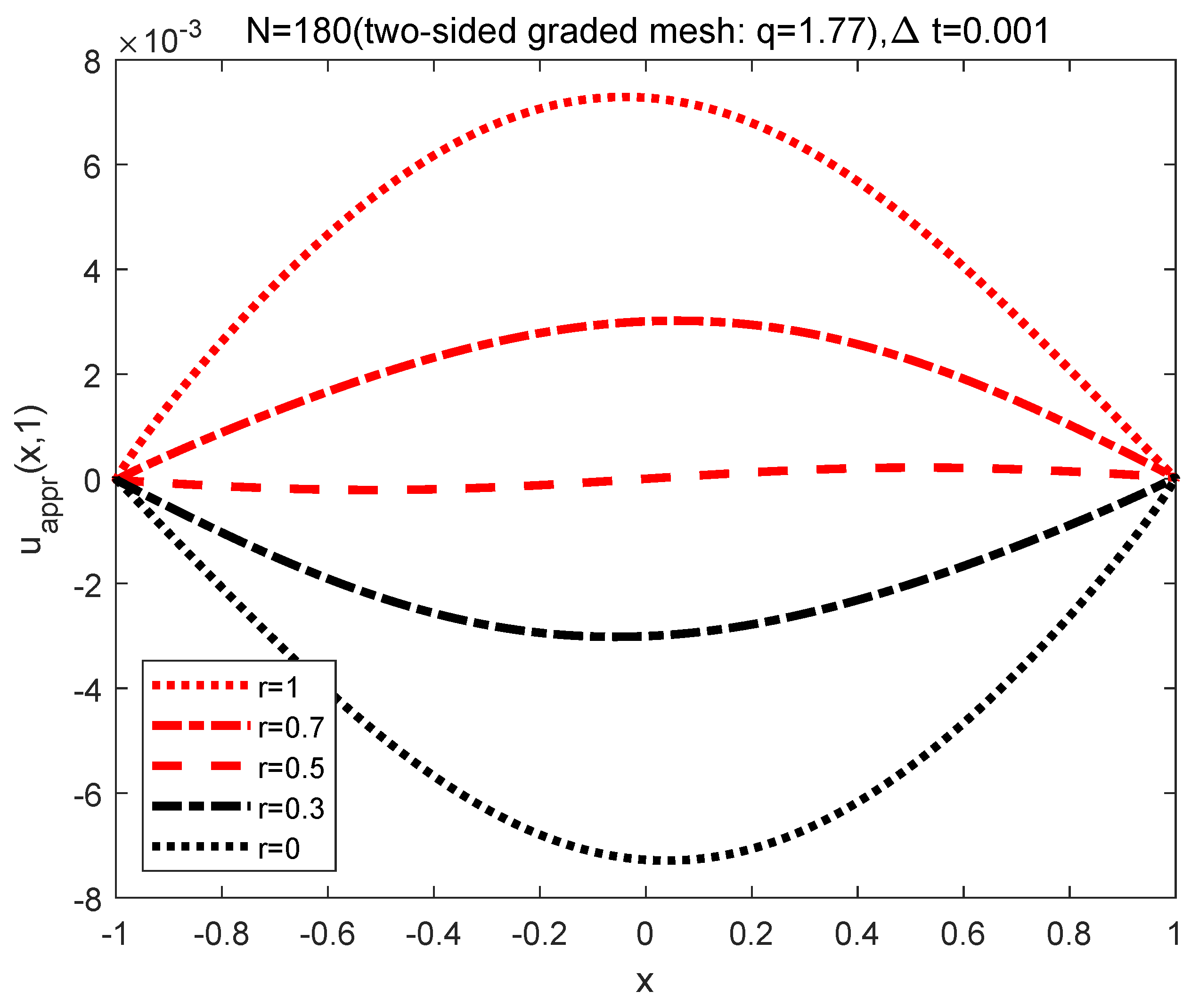
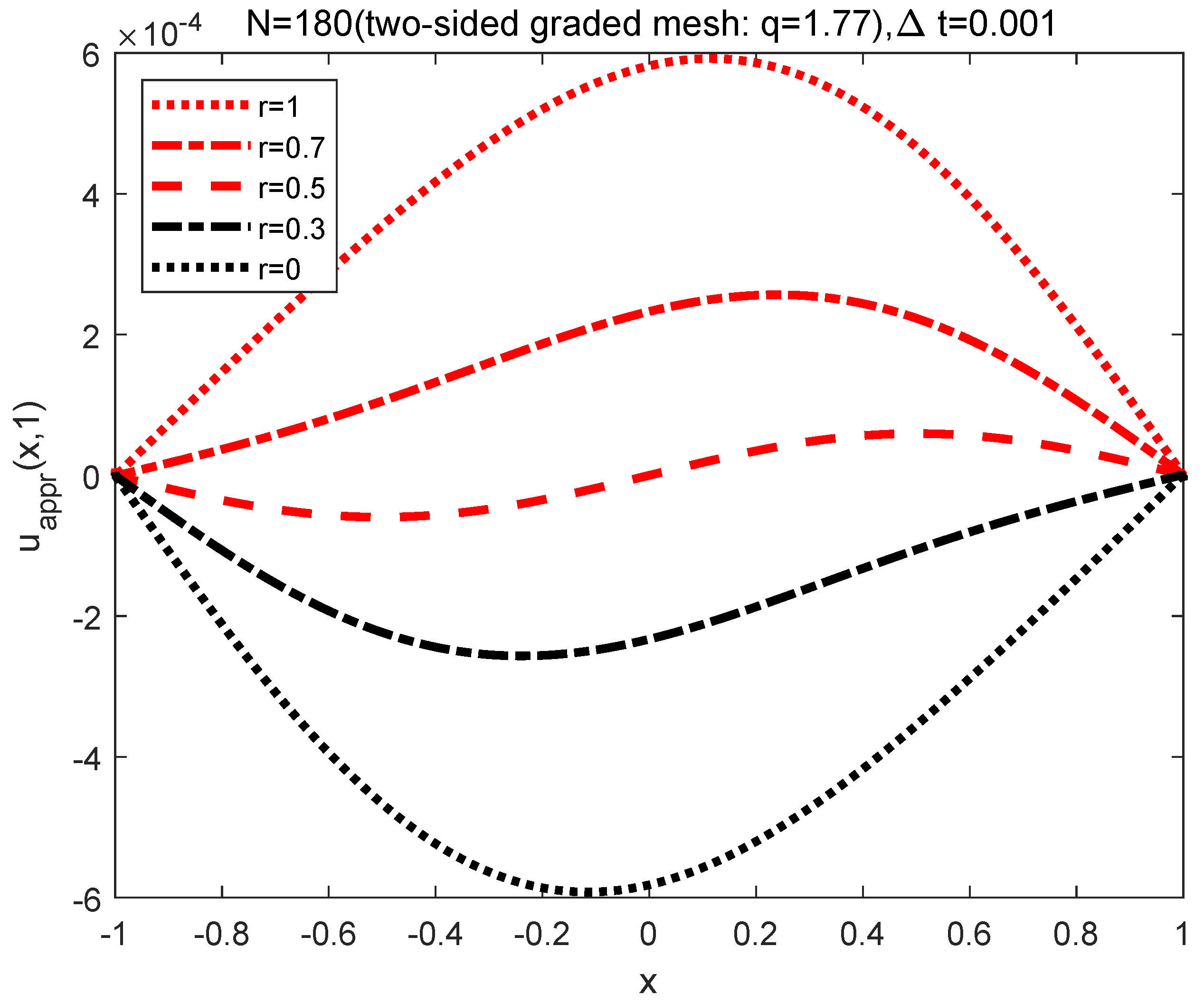
5.2. Fractional Burgers Equations

In this subsection, we try to solve the fractional Burgers equation as
t u ( x , t ) + u ( x , t ) x u ( x , t ) = ϵ D r α ( x , t ) u ( x , t ) ,
subject to homogeneous Dirichlet boundary condition and initial condition u ( x , 0 ) = u 0 ( x ) , where ϵ > 0 , 1 < α ( x , t ) < 2 and ( x , t ) ( 1 , 1 ) × ( 0 , 1 ] .
The two-step Crank-Nicolson/leapfrog scheme is first employed for time stepping, then the HCSCM is applied to the resulting equations. Thus, the full discretization scheme reads as: for k = 1 , 2 , ,
M Δ t ϵ D α k + 1 u k + 1 = g , M u 1 = M + Δ t ϵ D α 0 u 0 Δ t M u 0 . S u 0 M u 0 = u 0 ( x ) ,
where
g = M + Δ t ϵ D α k 1 u k 1 2 Δ t M u k . S u k ,
and Δ t is the time stepsize, M the collocation matrix, D α k the fractional differentiation matrix of order α k = α ( x , k Δ t ) with respect to the fractional operator D α ( x , t ) = D r α ( x , t ) as in (25), S the collocation first-order differentiation matrix which defines as
S = [ ϕ 0 ( x c ) , φ 1 ( x c ) , ϕ 1 ( x c ) , , φ N 1 ( x c ) , ϕ N 1 ( x c ) , ϕ N ( x c ) ] ,
and notation . the entry-to-entry multiplication.
Example 3.
In this example, we consider the fractional Burgers Equation (47) with the initial condition u 0 ( x ) = sin ( π x ) .
Our first test is the numerical solutions to the Equation (47) of the left Riemann-Liouville fractional derivative. The following five cases of fractional order are considered in [40,49]:
  • Case 1: (constant-order) α ( x , t ) = 1.1 , 1.2 , 1.3 , 1.5 , 1.8 ;
  • Case 2: (monotonic increasing-order) α ( x , t ) = 1 + 5 + 4 x 10 ;
  • Case 3: (monotonic decreasing-order) α ( x , t ) = 1 + 5 4 x 10 ;
  • Case 4: (nonsmooth order) α ( x , t ) = 1.1 + 4 5 | sin ( 10 π ( x t ) ) | ;
  • Case 5: (nonsmooth order) α ( x , t ) = 1.1 + 4 | x t | 5 .
In Figure 11, the numerical solutions at t = 1 is plotted for constant-order cases (Case 1). The obtained numerical result is the same as the one in Fig4.6 ([49]). We also compare some results by the multi-domain spectral collocation method(MDSCM) with those by the presented method(HCSCM) for α = 1.1 , 1.5 in Figure 12 and Figure 13. It is shown that by the HCSCM one get smoother numerical solution near the left boundary x = 1 than that by the MDSCM.
The numerical solutions at t = 1 for variable-order cases(Case 2–5) are plotted in Figure 14, Figure 15, Figure 16 and Figure 17, which are agree with the results in [40,49].
The numerical solutions are also computed to the fractional Burgers equation with two-sided operators. The numerical solutions at t = 1 for various α ’s and r’s are plotted in Figure 18, Figure 19, Figure 20, Figure 21, Figure 22 and Figure 23.

6. Conclusions

In this paper, a Hermite cubic spline collocation method (HCSCM) are developed for solving variable-order nonlinear fractional differential equations, which apply C 1 -continuous nodal basis functions to approximate problem. It is verified that the order of convergence of the HCSCM is O ( h min { 4 α , p } ) , while the interpolating function belongs to C p ( p 1 ) , where h is the mesh-size and α the order of the fractional derivative. The effectiveness of the HCSCM is demonstrated by solving fractional Helmholtz equations of constant-order and variable-order, and solving the fractional Burgers equation. The numerical fractional diffusions are compared with different senses.
The HCSCM can be applied to fractional-order differential equations on a two or three dimensional Descartes product domain by nodal basis tensor. Through adjusting the location of collocation points, the stability of the HCSCM can be observed numerically. Our future work will focus on the stability and error analysis of the HCSCM for some FDEs.

Author Contributions

Methodology, numerical tests and writing, T.Z.; review and editing, Y.W. All authors have read and agreed to the published version of the manuscript.

Funding

This research was funded by National Natural Science Foundation of China under Grant No. 11661048.

Institutional Review Board Statement

Not applicable.

Informed Consent Statement

Not applicable.

Data Availability Statement

Not applicable.

Conflicts of Interest

The authors declare no conflict of interest.

Abbreviations

The following abbreviations are used in this manuscript:
HCSCMHermite cubic spline collocation method
FDEsFractional differential equations
FDMFractional differentiation matrix
MDSCMMulti-domain spectral collocation method

References

  1. Metzler, R.; Klafter, J. The restaurant at the end of the random walk: Recent developments in the description of anomalous transport by fractional dynamics. J. Phys. A 2004, 37, 161–208. [Google Scholar] [CrossRef]
  2. Metzler, R.; Klafter, J. The random walk’s guide to anomalous diffusion: A fractional dynamics approach. Phys. Rep. 2000, 339, 1–77. [Google Scholar] [CrossRef]
  3. Rossikhin, Y.A.; Shitikova, M.V. Applications of fractional calculus to dynamic problems of linear and nonlinear hereditary mechanics of solids. Appl. Mech. Rev. 1997, 50, 15–67. [Google Scholar] [CrossRef]
  4. Mainardi, F. Fractional calculus: Some basic problems in continuum and statistical mechanics. In Fractals and Fractional Calculus in Continuum Mechenics; Carpinteri, A., Mainardi, F., Eds.; Springer: New York, NY, USA, 1997; pp. 291–348. [Google Scholar]
  5. Noeiaghdam, S.; Sidorov, D. Caputo-Fabrizio fractional derivative to solve the fractional model of energy supply-demand system. Math. Model. Eng. Probl. 2020, 7, 359–367. [Google Scholar] [CrossRef]
  6. Lin, Y.M.; Xu, C.J. Finite difference/spectral approxiamtions for the time-fractional diffusion equation. J. Comput. Phys. 2007, 225, 1533–1552. [Google Scholar] [CrossRef]
  7. Liu, F.; Anh, V.; Turner, I. Numerical solution of the space fractional Fokker-Planck equation. J. Comput. Appl. Math. 2004, 166, 209–219. [Google Scholar] [CrossRef] [Green Version]
  8. Meerschaert, M.M.; Scheffler, H.P.; Tadjeran, C. Finite difference methods for two-dimensional fractional dispersion equation. J. Comput. Phys. 2006, 211, 249–261. [Google Scholar] [CrossRef]
  9. Meerschaert, M.M.; Tadjeran, C. Finite difference approximations for fractional advection-dispersion flow equations. J. Comput. Appl. Math. 2004, 172, 65–77. [Google Scholar] [CrossRef] [Green Version]
  10. Sun, Z.Z.; Wu, X.N. A fully discrete difference scheme for a diffusion-wave system. Appl. Numer. Math. 2006, 56, 193–209. [Google Scholar] [CrossRef]
  11. Tadjeran, C.; Meerschaert, M.M.; Scheffler, H.P. A second-order accurate numerical approximation for the fractional diffusion equation. J. Comput. Phys. 2006, 213, 205–213. [Google Scholar] [CrossRef]
  12. Tadjeran, C.; Meerschaert, M.M. A second-order accurate numerical method for the two-dimensional fractional diffusion equation. J. Comput. Phys. 2007, 220, 813–823. [Google Scholar] [CrossRef]
  13. Wang, H.; Basu, T.S. A fast finite difference method for two-dimensional space-fractional diffusion equation. SIAM J. Sci. Comput. 2012, 34, 2444–2458. [Google Scholar] [CrossRef]
  14. Wang, H.; Wang, K. An O(Nlog2N) alternating-direction finite difference method for two-dimensional fractional diffusion equation. J. Comput. Phys. 2011, 230, 7830–7839. [Google Scholar] [CrossRef]
  15. Zhang, Y.; Sun, Z.Z.; Wu, H.W. Error estimates of Crank-Nicolson type difference schemes for the sub-diffusion eqution. SIAM J. Numer. Anal. 2011, 49, 2302–2322. [Google Scholar] [CrossRef]
  16. Zhou, H.; Tian, W.Y.; Deng, W.H. Quasi-compact finite difference schemes for space fractional diffusion equations. J. Sci. Comput. 2013, 56, 45–66. [Google Scholar] [CrossRef] [Green Version]
  17. Zhao, X.; Sun, Z.Z.; Hao, Z.P. A fourth-order compact ADI scheme for two-dimensional nonlinear space fractional Schrödinger equation. SIAM J. Sci. Comput. 2014, 36, A2865–A2886. [Google Scholar] [CrossRef]
  18. Deng, W.H. Finite element method for the space and time fractional Fokker-Planck equation. SIAM J. Numer. Anal. 2008, 47, 204–226. [Google Scholar] [CrossRef]
  19. Ford, N.; Xiao, J.Y.; Yan, Y.B. A finite element method for time fractional partial differential equations. Fract. Calc. Appl. Anal. 2011, 14, 454–474. [Google Scholar] [CrossRef] [Green Version]
  20. Jiang, Y.; Ma, J. High-order finite element methods for time-fractional partial differential equations. J. Comput. Appl. Math. 2011, 235, 3285–3290. [Google Scholar] [CrossRef] [Green Version]
  21. Lian, Y.; Ying, Y.; Tang, S.; Lin, S.; Wagner, G.J.; Liu, W.K. A Petrev-Galerkin finite element method for the fractional advection-diffusion equation. Comput. Methods Appl. Mech. Engrg. 2016, 309, 388–410. [Google Scholar] [CrossRef]
  22. Wang, H.; Yang, D.P.; Zhu, S.F. A Petrev-Galerkin finite element method for variable-coefficient fractional diffusion equations. Comput. Methods Appl. Mech. Engrg. 2015, 290, 45–56. [Google Scholar] [CrossRef]
  23. Zheng, Y.Y.; Li, C.P.; Zhao, Z.G. A note on the finite element method for the space-fractional advection diffusion equation. Comput. Math. Appl. 2010, 59, 1718–1726. [Google Scholar] [CrossRef] [Green Version]
  24. Li, C.P.; Zeng, F.H.; Liu, F. Spectral approximations to the fractional integral and derivative. Fract. Calc. Appl. Anal. 2012, 15, 383–406. [Google Scholar] [CrossRef] [Green Version]
  25. Li, X.J.; Xu, C.J. A space-time spectral method for the time fractional diffusion equations. SIAM J. Numer. Anal. 2009, 47, 2018–2131. [Google Scholar] [CrossRef]
  26. Li, X.J.; Xu, C.J. Existence and uniqueness of the weak solution of the space-time fractional diffusion equation and a spectral method approximation. Commun. Comput. Phys. 2010, 8, 1016–1051. [Google Scholar]
  27. Tian, W.Y.; Deng, W.H.; Wu, Y.J. Polynomial spectral collocation method for space fractional advection-diffusion equation. Numer. Methods Partial Differ. Eq. 2014, 30, 514–535. [Google Scholar] [CrossRef] [Green Version]
  28. Xu, Q.W.; Hesthaven, J.S. Stable multi-domian spectral penalty methods for fractional partial differential equations. J. Comput. Phys. 2014, 257, 241–258. [Google Scholar] [CrossRef] [Green Version]
  29. Mao, Z.P.; Chen, S.; Shen, J. Efficient and accurate spectral method using generalized Jacobi functions for solving Riesz fractional differential equations. Appl. Numer. Math. 2016, 106, 165–181. [Google Scholar] [CrossRef]
  30. Mao, Z.P.; Shen, J. Efficient spectral-Galerkin methods for fractional partial differential equations with variable coefficients. J. Comput. Phys. 2016, 307, 243–261. [Google Scholar] [CrossRef] [Green Version]
  31. Zeng, F.H.; Liu, F.W.; Li, C.P.; Burrage, K.; Turner, I.; Anh, V. A Crank-Nicolson ADI spectral method for a two-dimensional Riesz space fractional nonlinear reaction-diffusion equation. SIAM J. Numer. Anal. 2014, 52, 2599–2622. [Google Scholar] [CrossRef] [Green Version]
  32. Zayernouri, M.; Karniadakis, G.E. Discontinuous spectral element methods for time- and space-fractional advection equations. SIAM J. Sci. Comput. 2014, 36, B684–B707. [Google Scholar] [CrossRef]
  33. Kharazmi, E.; Zayernouri, M.; Karniadakis, G.E. A Petrov-Galerkin spectral element method for fractional elliptic problems. Comput. Methods Appl. Mech. Engrg. 2017, 324, 512–536. [Google Scholar] [CrossRef] [Green Version]
  34. Li, C.P.; Cai, M. Theory and Numerical Approximations of Fractional Integrals and Derivatives; SIAM: Philadelphia, PA, USA, 2020. [Google Scholar]
  35. Shen, J.; Tang, T.; Wang, L.L. Spectral Methods: Algorithms, Analysis and Applications; Springer: Berlin/Heidelberg, Germany, 2011. [Google Scholar]
  36. Guo, B.Y. The Spectral Methods and Its Applications; World Scientific: Singapore, 1998. [Google Scholar]
  37. Bernardi, C.; Maday, Y. Spectral methods. In Handbook of Numerical Analysis, Vol. V, Techniques of Scientific Computing (Part 2); Ciarlet, P.G., Lions, J.L., Eds.; Elsevier: Amsterdam, The Netherlands, 1997; pp. 209–486. [Google Scholar]
  38. Boyd, J.P. Chebyshev and Fourier Spectral Methods, 2nd ed.; Dover Publication: Mineola, NY, USA, 2000. [Google Scholar]
  39. Chen, S.; Shen, J.; Wang, L.L. Generalized Jacobi functions and their applications to fractional differential equations. Math. Comput. 2016, 85, 1603–1638. [Google Scholar] [CrossRef] [Green Version]
  40. Zeng, F.H.; Zhang, Z.Q.; Karniadakis, G.E. A generalized spectral collocation method with tunable accuracy for variable-order fractional differential equations. SIAM J. Sci. Comput. 2015, 37, A2710–A2732. [Google Scholar] [CrossRef]
  41. Zeng, F.H.; Mao, Z.P.; Karniadakis, G.E. A generalized spectral collocation method with tunable accuracy for fractional differential equations with end-point singularities. SIAM J. Sci. Comput. 2017, 39, A360–A383. [Google Scholar] [CrossRef] [Green Version]
  42. Mao, Z.P.; Karniadakis, G.E. A spectral method (of exponential convergence) for singular solutions of the diffusion equation with general two-sided fractional derivative. SIAM J. Numer. Anal. 2018, 56, 24–49. [Google Scholar] [CrossRef]
  43. Zayernouri, M.; Karniadakis, G.E. Fractional Sturm-Liouville eigenproblems: Theory and numerical approximation. J. Comput. Phys. 2013, 252, 495–517. [Google Scholar] [CrossRef]
  44. Zayernouri, M.; Karnidakis, G.E. Fractional spectral collocation method. SIAM J. Sci. Comput. 2014, 36, A40–A62. [Google Scholar] [CrossRef]
  45. Zayernouri, M.; Karnidakis, G.E. Fractional spectral collocation methods for linear and nonlinar variable order FPDEs. J. Comput. Phys. 2015, 293, 312–338. [Google Scholar] [CrossRef] [Green Version]
  46. Huang, C.; Jiao, Y.J.; Wang, L.L.; Zhang, Z.M. Optimal fractional integration preconditioning and error analysis of fractional collocation method using nodal generalised Jacobi functions. SIAM J. Numer. Anal. 2016, 54, 3357–3387. [Google Scholar] [CrossRef]
  47. Jiao, Y.J.; Wang, L.L.; Huang, C. Well-conditioned fractional collocation methods using fractional Birkhoff interpolation basis. J. Comput. Phys. 2016, 305, 1–28. [Google Scholar] [CrossRef] [Green Version]
  48. Zhang, Z.Q.; Zeng, F.H.; Karniadakis, G.E. Optimal error estimates of spectral petrov-Galerkin and collocation methods for initial value problems of fractional differential equations. SIAM J. Numer. Anal. 2015, 53, 2074–2096. [Google Scholar] [CrossRef]
  49. Zhao, T.G.; Mao, Z.P.; Karniadakis, G.E. Multi-domain spectral collocation method for variable-order nonlinear fractional differential equations. Comput. Methods Appl. Mech. Engrg. 2019, 348, 377–395. [Google Scholar] [CrossRef] [Green Version]
  50. Bialecki, B.; Fairweather, G. Orthogonal spline collocation methods for partial differential equations. J. Comput. Appl. Math. 2001, 128, 55–82. [Google Scholar] [CrossRef] [Green Version]
  51. Douglas, J., Jr.; Dupont, T. Collocation methods for parabolic equations in a single space variable. In Lecture Notes in Mathematics; Springer: New York, NY, USA, 1974; Volume 385. [Google Scholar]
  52. Greenwell-Yanik, C.E.; Fairweather, G. Analyses of spline collocation methods for parabolic and hyperbolic problems in two space variables. SIAM J. Numer. Anal. 1986, 23, 282–296. [Google Scholar] [CrossRef]
  53. Liu, J.; Fu, H.F.; Chai, X.C.; Sun, Y.N.; Guo, H. Stability and convergence analysis of the quadratic spline collocation method for time-dependent fractional diffusion equations. Appl. Math. Comput. 2019, 346, 633–648. [Google Scholar] [CrossRef]
  54. Majeed, A.; Kamran, M.; Iqbal, M.K.; Baleanu, D. Solving time fractional Burgers’ and Fisher’s equations using cubic B-spline approximation method. Adv. Diff. Equ. 2020, 2020, 175. [Google Scholar] [CrossRef]
  55. Khalid, N.; Abbas, M.; Iqbal, M.K. Non-polynomial quintic spline for solving fourth-order fractional boundary value problems involving product terms. Appl. Math. Comput. 2019, 349, 393–407. [Google Scholar] [CrossRef]
  56. Emadifar, H.; Jalilian, R. An exponential spline approximation for fractional Bagley-Torvik equation. Bound. Value Probl. 2020, 2020, 20. [Google Scholar] [CrossRef]
  57. Kilbas, A.A.; Srivastava, H.M.; Trujillo, J.J. Theory and Applications of Fractional Differential Equations; Elsevier Science: Amsterdam, The Netherlands, 2006. [Google Scholar]
  58. Podlubny, I. Fractional Differential Equations: An Introduction to Fractional Derivatives, Fractional Differential Equations, to Methods of Their Solution and some of Their Applications; Mathematics in Science and Engineering; Academic Press: San Diego, CA, USA, 1999; Volume 198. [Google Scholar]
  59. Patie, P.; Simon, T. Intertwining certain fractional derivatives. Potential Anal. 2012, 36, 569–587. [Google Scholar] [CrossRef] [Green Version]
  60. Sun, W. The spectral analysis of Hermite cubic spline collocation systems. SIAM J. Numer. Anal. 1999, 36, 1962–1975. [Google Scholar] [CrossRef]
  61. Sun, W. Hermite cubic spline collocation method with upwind features. ANZIAM J. 2000, 42, C1379–C1397. [Google Scholar] [CrossRef] [Green Version]
  62. Varma, A.K.; Howell, G. Best error bounds for derivatives in two point Birkhoff interpolation problems. J. Approx. Theory 1983, 38, 258–268. [Google Scholar] [CrossRef] [Green Version]
  63. Birkhoff, G.; Schultz, M.H.; Varga, R.S. Piecewise Hermite interpolation in one and two variables with applications to partial differential equations. Numer. Math. 1968, 11, 232–256. [Google Scholar] [CrossRef]
Figure 1. Error for Example 1 with Mesh 1: α ( x ) = 1.1 , 1.5 , 1.9 .
Symmetry 13 00872 g001
Figure 2. Error for Example 1 with Mesh 1: α ( x ) = 1.1 + x + 1 2.5 .
Symmetry 13 00872 g002
Figure 3. Error for Example 2 with exact solution: u ( x ) = ( 1 x ) ( 1 + x ) α ( x ) and ( σ 1 , σ 2 ) = ( 3 3 , 1 3 3 ) . Mesh 1 for α = 1.1 , 1.5 , 1.9 .
Symmetry 13 00872 g003
Figure 4. Error for Example 2 with exact solution: u ( x ) = ( 1 x ) ( 1 + x ) α ( x ) and ( σ 1 , σ 2 ) = ( 3 3 , 1 3 3 ) .
Symmetry 13 00872 g004
Figure 5. Error for Example 2 with exact solution: u ( x ) = ( 1 x ) ( 1 + x ) α ( x ) and ( σ 1 , σ 2 ) = ( 3 3 , 1 3 3 ) of left Caputo case ( α = 1.1 ).
Symmetry 13 00872 g005
Figure 6. Error for Example 2 with exact solution: u ( x ) = ( 1 x ) ( 1 + x ) α ( x ) and ( σ 1 , σ 2 ) = ( 3 3 , 1 3 3 ) of left Patie-Simon( α = 1.1 ).
Symmetry 13 00872 g006
Figure 7. Error for Example 2 with exact solution u ( x ) = ( 1 x ) ( 1 + x ) α ( x ) 1 and ( σ 1 , σ 2 ) = ( 3 3 , 1 3 3 ) by the uniform mesh.
Symmetry 13 00872 g007
Figure 8. Error for Example 2 with exact solution: u ( x ) = ( 1 x ) ( 1 + x ) α ( x ) 1 and ( σ 1 , σ 2 ) = ( 3 3 , 1 3 3 ) .
Symmetry 13 00872 g008
Figure 9. Error for Example 2 with exact solution u ( x ) = ( 1 x ) ( 1 + x ) α ( x ) 1 and λ = 0 , ( σ 1 , σ 2 ) = ( 3 3 , 1 3 3 ) of left Riemann-Liouville with constant-order case.
Symmetry 13 00872 g009
Figure 10. Error for Example 2 with exact solution u ( x ) = ( 1 x ) ( 1 + x ) α ( x ) 1 and λ = 0 , ( σ 1 , σ 2 ) = ( 3 3 , 1 3 3 ) of left Riemann-Liouville with variable-order case.
Symmetry 13 00872 g010
Figure 11. Numerical solutions at t = 1 for Example 3 (Case 1) with the graded mesh (Mesh 2). ϵ = 1 , N = 200 , Δ t = 10 3 and ( σ 1 , σ 2 ) = ( 0.09 , 0.88 ) for α = 1.1 , 1.3 , ( σ 1 , σ 2 ) = ( 0.09 , 0.85 ) for α = 1.2 , ( σ 1 , σ 2 ) = ( 0.3 , 0.7 ) for α = 1.5 , 1.8 .
Symmetry 13 00872 g011
Figure 12. Numerical solutions at t = 1 for Example 3 with left Riemann-Liouville case( α = 1.1 , r = 1 ): MDSCM vs HCSCM. ( σ 1 , σ 2 ) = ( 0.09 , 0.88 ) for N = 200 , 400 and the two-sided graded mesh (Mesh 2) are used for all cases in HCSCM.
Symmetry 13 00872 g012
Figure 13. Numerical solutions at t = 1 for Example 3 with left Riemann-Liouville case( r = 1 , α = 1.5 ): MDSCM vs HCSCM. ( σ 1 , σ 2 ) = ( 0.2 , 0.7 ) for N = 50 , 100 , 200 and the two-sided graded mesh (Mesh 2) are used for all cases in HCSCM.
Symmetry 13 00872 g013
Figure 14. Numerical solutions at t = 1 for Example 3 with left Riemann-Liouville case ( r = 1 ) and ϵ = 1 : α ( x ) = 1 + 5 + 4 x 10 .
Symmetry 13 00872 g014
Figure 15. Numerical solutions at t = 1 for Example 3 with left Riemann-Liouville case ( r = 1 ) and ϵ = 1 : α ( x ) = 1 + 5 4 x 10 .
Symmetry 13 00872 g015
Figure 16. Numerical solutions at t = 1 for Example 3 with left Riemann-Liouville case ( α ( x , t ) = 1.1 + 4 5 | sin ( 10 π ( x t ) ) | , r = 1 ) and ϵ = 1 . where ( σ 1 , σ 2 ) = ( 0.35 , 0.85 ) for N = 50 , ( σ 1 , σ 2 ) = ( 0.28 , 0.75 ) for N = 100 , ( σ 1 , σ 2 ) = ( 0.2 , 0.75 ) for N = 200 .
Symmetry 13 00872 g016
Figure 17. Numerical solutions at t = 1 for Example 3 with left Riemann-Liouville case ( α ( x , t ) = 1.1 + 4 | x t | 5 , r = 1 ) and ϵ = 1 . where ( σ 1 , σ 2 ) = ( 0.2 , 0.75 ) for all three Ns.
Symmetry 13 00872 g017
Figure 18. Numerical solutions at t = 1 for Example 3 of two-sided Riemann-Liouville case ( r = 0.3 ): ϵ = 1 , ( σ 1 , σ 2 ) = ( 3 3 , 1 3 3 ) for all cases.
Symmetry 13 00872 g018
Figure 19. Numerical solutions at t = 1 for Example 3 of two-sided Riemann-Liouville case ( r = 0.5 ): ϵ = 1 , ( σ 1 , σ 2 ) = ( 3 3 , 1 3 3 ) for all cases.
Symmetry 13 00872 g019
Figure 20. Numerical solutions at t = 1 for Example 3 of two-sided Riemann-Liouville case ( α = 1.22 ): ϵ = 1 , ( σ 1 , σ 2 ) = ( 3 3 , 1 3 3 ) for all cases.
Symmetry 13 00872 g020
Figure 21. Numerical solutions at t = 1 for Example 3 of two-sided Riemann-Liouville case ( α = 1.5 ): ϵ = 1 , ( σ 1 , σ 2 ) = ( 3 3 , 1 3 3 ) for all cases.
Symmetry 13 00872 g021
Figure 22. Numerical solutions at t = 1 for Example 3 of two-sided Riemann-Liouville case ( α = 1.9 ): ϵ = 1 , ( σ 1 , σ 2 ) = ( 3 3 , 1 3 3 ) for all cases.
Symmetry 13 00872 g022
Figure 23. Numerical solutions at t = 1 for Example 3 of two-sided Riemann-Liouville case ( α = 1.99 ): ϵ = 1 , ( σ 1 , σ 2 ) = ( 3 3 , 1 3 3 ) for all cases.
Symmetry 13 00872 g023
Table 1. Error E 0 and the order of convergence (OC), for Example 1 with Mesh 1: α ( x ) = 1.2 , 1.4 , 1.6 , 1.8 , ( σ 1 , σ 2 ) = ( 0.2 , 0.8 ) , λ = 0 .
N α ( x ) = 1.2 OC α ( x ) = 1.4 OC α ( x ) = 1.6 OC α ( x ) = 1.8 OC
201.1797 × 10 4 -1.1326 × 10 4 -1.8116 × 10 4 -2.9010 × 10 4 -
401.6776 × 10 5 2.811.7641 × 10 5 2.683.3277 × 10 5 2.456.2240 × 10 5 2.22
802.4257 × 10 6 2.792.8890 × 10 6 2.616.2306 × 10 6 2.421.3406 × 10 5 2.22
1207.8179 × 10 7 2.791.0058 × 10 6 2.602.3442 × 10 6 2.415.4714 × 10 6 2.21
1603.5026 × 10 7 2.794.7588 × 10 7 2.601.1740 × 10 6 2.402.8984 × 10 6 2.21
2001.8588 × 10 7 2.842.6617 × 10 7 2.606.8516 × 10 7 2.411.7712 × 10 6 2.21
2401.1199 × 10 7 2.781.6566 × 10 7 2.604.4209 × 10 7 2.401.1876 × 10 6 2.19
Table 2. Error E 0 and the CPU time for Example 1 with Mesh 1: α = 1.4 , ( σ 1 , σ 2 ) = ( 0.2 , 0.8 ) , λ = 0 .
N E 0 CPU Time (s)
103.6097 × 10 3 0.018
508.8401 × 10 5 0.165
1001.5063 × 10 5 0.479
1505.2966 × 10 6 1.046
2002.5185 × 10 6 1.831
2501.4119 × 10 6 2.721
3008.8569 × 10 7 3.397
5002.3094 × 10 7 7.363
10001.0710 × 10 7 23.029
Table 3. Error E 0 and the order of convergence (OC) for Example 2 with Mesh 1: α ( x ) = 1.2 , 1.4 , 1.6 , 1.8 , ( σ 1 , σ 2 ) = ( 0.2 , 0.8 ) , λ = 0 .
N α ( x ) = 1.2 OC α ( x ) = 1.4 OC α ( x ) = 1.6 OC α ( x ) = 1.8 OC
203.6965 × 10 3 -3.5347 × 10 3 -1.9174 × 10 3 -5.9525 × 10 4 -
401.6497 × 10 3 1.161.3360 × 10 3 1.406.3033 × 10 4 1.601.6984 × 10 4 1.81
807.2079 × 10 4 1.195.0527 × 10 4 1.402.0733 × 10 4 1.604.8498 × 10 5 1.81
1204.4317 × 10 4 1.202.8620 × 10 4 1.401.0824 × 10 4 1.602.3318 × 10 5 1.81
1603.1379 × 10 4 1.201.9124 × 10 4 1.406.8268 × 10 5 1.601.3874 × 10 5 1.80
2002.4007 × 10 4 1.201.3990 × 10 4 1.404.7751 × 10 5 1.609.2759 × 10 6 1.80
2401.9289 × 10 4 1.201.0836 × 10 4 1.403.5659 × 10 5 1.606.6766 × 10 6 1.80
Table 4. Error E 0 and the order of convergence (OC) for Example 2 with Mesh 1: α ( x ) = 1.2 , 1.4 , 1.6 , 1.8 , ( σ 1 , σ 2 ) = ( 0.2 , 0.8 ) , λ = 0 .
N α ( x ) = 1.2 OC α ( x ) = 1.4 OC α ( x ) = 1.6 OC α ( x ) = 1.8 OC
201.1624 × 10 + 0 -4.0781 × 10 1 -1.0764 × 10 1 -1.8809 × 10 2 -
401.0453 × 10 + 0 0.153.1153 × 10 1 0.397.1834 × 10 2 0.581.0960 × 10 2 0.78
809.1739 × 10 1 0.192.3697 × 10 1 0.394.7653 × 10 2 0.596.3385 × 10 3 0.79
1208.4738 × 10 1 0.202.0173 × 10 1 0.403.7430 × 10 2 0.604.5930 × 10 3 0.79
1608.0061 × 10 1 0.201.7991 × 10 1 0.403.1524 × 10 2 0.603.6528 × 10 3 0.80
2007.6601 × 10 1 0.201.6460 × 10 1 0.402.7588 × 10 2 0.603.0577 × 10 3 0.80
2407.3879 × 10 1 0.201.5306 × 10 1 0.402.4738 × 10 2 0.602.6439 × 10 3 0.80
Publisher’s Note: MDPI stays neutral with regard to jurisdictional claims in published maps and institutional affiliations.

