Solutions to Nonlinear Evolutionary Parabolic Equations of the Diffusion Wave Type

Abstract

The article deals with nonlinear second-order evolutionary partial differential equations (PDEs) of the parabolic type with a reasonably general form. We consider the case of PDE degeneration when the unknown function vanishes. Similar equations in various forms arise in continuum mechanics to describe some diffusion and filtration processes as well as to model heat propagation in the case when the properties of the process depend significantly on the unknown function (concentration, temperature, etc.). One of the exciting and meaningful classes of solutions to these equations is diffusion (heat) waves, which describe the propagation of perturbations over a stationary (zero) background with a finite velocity. It is known that such effects are atypical for parabolic equations; they arise as a consequence of the degeneration mentioned above. We prove the existence theorem of piecewise analytical solutions of the considered type and construct exact solutions (ansatz). Their search reduces to the integration of Cauchy problems for second-order ODEs with a singularity in the term multiplying the highest derivative. In some special cases, the construction is brought to explicit formulas that allow us to study the properties of solutions. The case of the generalized porous medium equation turns out to be especially interesting as the constructed solution has the form of a soliton moving at a constant velocity.

1. Introduction

Parabolic partial differential equations (PDEs) are meaningful mathematical objects with non-trivial properties; they have been intensely studied in the scientific literature. There are, without exaggeration, thousands of articles and monographs that touch on various aspects of PDEs. We point out only three classical monographs that have significantly influenced the development of the theory of nonlinear parabolic equations [1,2,3].

This article is devoted to constructing and studying one special class of solutions to second-order nonlinear evolutionary parabolic equations. We consider the equation with the form

$$c_t={({\Phi }_1(c))}_{xx}+{({\Phi }_2(c))}_x+{\Phi }_3(c).$$

(1)

where $t,x$ are independent variables—t is time, x is a spatial variable—$c(t,x)$ is an unknown function, and ${\Phi }_i,i=1,2,3$ are the specified functions.

Equation (1) cannot be directly applied as a mathematical model of any particular process as it is written in a very general form. However, its special cases are widely known and popular models of continuum mechanics and describe various thermal, convective, and diffusion processes. Perhaps the most famous particular case is the porous medium equation [4], which corresponds to the case where ${\Phi }_1$ is a power function and ${\Phi }_2={\Phi }_3\equiv 0$. It is rich in applications and describes the filtration of an ideal gas in porous formations [5], as well as the radiant (nonlinear) thermal conductivity [6]. Therefore, in the Russian mathematical literature, it is often called the nonlinear heat equation. It is also successfully used in population dynamics modeling [7].

The second most common case is when ${\Phi }_1$ and ${\Phi }_3$ are power functions and ${\Phi }_2\equiv 0$. Then, (1) becomes the generalized porous medium equation [4]; it is also called “the nonlinear heat equation with a source” in the Russian literature [8]. This equation describes the same processes as the porous medium equation, but the model becomes more complex and allows us to take into account the inflow or outflow of matter or heat.

If ${\Phi }_3\equiv 0$, and ${\Phi }_1$ and ${\Phi }_2$ are nonzero, Equation (1) is called “the convection–diffusion equation” [9,10]. Several mathematical models of fluid mechanics that simultaneously describe the diffusion and convective [11] mechanisms of energy and matter transfer are reduced to this equation. Its particular case is the well-known Burgers equation [4]. Finally, Equation (1), if ${\Phi }_2(c)$ is a linear function, describes the non-stationary thermal conductivity in a medium moving at a constant speed, when the thermal conductivity coefficient and the reaction rate are arbitrary functions of the temperature [12]. The list could be continued, so the study of Equation (1) is still relevant.

Obviously, if ${\Phi }_3(0)=0$, then (1) has a trivial solution: $c\equiv 0$. A special feature of equations of this type is as follows: they can have solutions that describe perturbations that propagate at a finite velocity over a stationary (zero) background. Such solutions are usually called heat or diffusion waves depending on which physical process describes the equation. It is known that such effects, generally speaking, are atypical for parabolic PDEs [13].

Apparently, the first solutions of the porous medium equation with the type of a diffusion (heat) wave were obtained in the 1940s when studying the processes occurring after a nuclear explosion. The so-called Zel’dovich–Kompaneets solution was presented in 1950 in Russian. The English version of this paper appeared much later [6]. The same solutions were used to describe diffusion processes in the ground [5]; the results were first published in Russian in 1952.

A new stage in the study of solutions to nonlinear parabolic equations with the diffusion wave type began in the 1980s and 1990s when the monographs by A. Friedman [14] and A. A. Samarskii (with co-authors) [8] were published. The monographs were not entirely devoted to constructing and investigating such solutions, but the corresponding results were obtained as auxiliary results. We highlight the results of A. F. Sidorov in the 1980s, who constructed solutions to some initial boundary value problems generating diffusion waves in the class of analytical functions [15]. In the Russian mathematical literature in the 21st century, this problem is sometimes referred to as Andrei Sakharov’s problem. Somewhat later, but independently, similar results were obtained by S. Angenent [16]. Then, the research of A.F. Sidorov was continued by his students [17], including the author of this article. In 2013, we published an article in which the questions that had previously remained open were closed; the main question was whether the constructed series converge [18]. The existence and uniqueness theorem of the solution of the problem of the initiation of a diffusion wave for the porous medium equation in the case of plane symmetry was proved. The theorem is an analog of the classical Cauchy–Kovalevskaya theorem [19] for the considered case.

Further, these results were extended to the cases of circular and spherical symmetry [20] and to the two-dimensional case [21,22], as well as to the case of the simplest nonlinear systems [23]. Since the proved theorems are local, as with all such statements, starting with the Cauchy–Kovalevskaya theorem, the question of the domain of the solution’s existence is relevant. In the general case, it seems to be possible to find the answer only numerically. Therefore, we developed a numerical-analytical method based on the well-known boundary element method (BEM) [24,25] using the dual reciprocity method [26]. BEM algorithms were developed and implemented to solve various initial-boundary value problems, the solutions of which have the form of a diffusion (heat) wave. The cases of one [20,27] and two spatial variables [28] are considered, while the segments of special series [29] are used to eliminate the singularity, and the previously obtained explicit analytical formulas [30] are applied to calculate the integrals.

All the proposed computational algorithms are heuristic, and their convergence could not be proved; however, this is typical for nonlinear singular PDEs. In such a situation, the issue of verifying the results of calculations becomes particularly relevant. One effective method is to compare numerical results with exact solutions. In the literature, we managed to find a relatively small number of solutions of the desired type, although, in general, quite a large number of exact solutions for the porous medium equation and generalized porous medium equation are known [12]. In such a situation, we made efforts to find exact solutions to these equations using group analysis methods [31], and various types of ansatzes [12]. In some cases, the construction was brought to an explicit formula, but usually we reduce it to Cauchy problems for ODEs with singularities in terms that multiply the highest derivative [32,33,34].

C. Foias and co-authors introduced the concept of an inertial manifold for nonlinear evolutionary equations; in particular, for parabolic equations. These manifolds contain the global attractor, they attract all solutions exponentially, and they are stable to perturbations. In the infinite-dimensional case, they reduce the dynamics to a finite-dimensional ODE [35] (see also [36]). These results were expanded to parabolic equations and systems in [37].

In the 21st century, a large number of publications have appeared that concern the asymptotic properties of solutions to parabolic-type equations and systems. Let us mention, for example, the work in [38], which considers, among other things, equations of the form close to (1) and provides an extensive bibliography. Of the recent publications, we can mention the work in [39], which is devoted to studying the asymptotic behavior of solutions for a class of nonclassical diffusion equations in a smooth bounded domain with a dynamic boundary condition.

Special mention in the context of this paper should be paid to the studies of S.N. Antontsev and S.I. Shmarev, who consider problems with a free boundary for nonlinear parabolic equations in general formulations in abstract functional spaces [40,41]. We also allude to A.A. Kosov and E.I. Semenov, who construct exact solutions for equations of the considered type that are not diffusion waves [42], and I.V. Stepanova, who deals with modeling heat and mass transfer using nonlinear parabolic systems [43,44].

In this paper, our previous studies are developed and expanded for a new class. The key results are as follows. First, we prove a new existence and uniqueness theorem for the problem of a diffusion wave motion with a specified front for Equation (1). The theorem is an analog of the Cauchy–Kovalevskaya theorem for the case considered. Second, we construct an example that is analogous to the example of Kovalevskaya. Finally, in the most interesting particular cases for applications, exact solutions to Equation (1) that have the diffusion wave type are constructed. We investigate the asymptotic behavior of solutions and show that one of them is a soliton. To the best of our knowledge, the results are new for a problem with such a general formulation. At the same time, this was necessary to obtain a flexible and versatile tool for studying the properties of the generalized model under consideration (see Section 6 and Section 7).

2. Formulation

If the functions ${\Phi }_1(c),{\Phi }_2(c)$ are differentiable, then Equation (1) can be rewritten as

$$c_t={({\Phi }_1^{\prime }(c)c_x)}_x+{\Phi }_2^{\prime }(c)c_x+{\Phi }_3(c).$$

(2)

In turn, if the function $K(c)={\Phi }_1^{\prime }(c)$ is sufficiently smooth and monotonic, after the substitution $u=K(c)$, Equation (2) can be reduced (by trivial transformations) to the form

$$u_t=u{u}_{xx}+f(u)u_x^2+g(u)u_x+h(u).$$

(3)

where $f(u)=u{\varphi }^{″}(u)/{\varphi }^{\prime }(u)+1$, $g(u)={\Phi }_2^{\prime }(\varphi (u))$, $h(u)={\Phi }_3(\varphi (u))/{\varphi }^{\prime }(u)$, $K(\varphi (u))=u$, i.e., $\varphi (u)$ is the inverse function to $K(c)$.

Consider the boundary condition:

$${u(t,x)|}_{x=a(t)}=0.$$

(4)

Problem (3), (4) is untypical for second-order equations. It includes only one boundary condition for the unknown function, which causes the term multiplying the higher derivative to vanish. Thus, the classical existence and uniqueness theorems do not work in this case. Nevertheless, the existence and uniqueness theorem of a nontrivial solution is valid. We formulate and prove this in the next section.

3. Existence Theorem

Let us formulate and prove the existence theorem of locally analytical solutions to problem (3), (4). Here and in the following, an analytical function at the point means a function that coincides in a neighborhood with its Taylor expansion. To simplify the terminology, we will use the term “analytical at the point”.

Theorem 1.

Let $a(t)$, $f(u)$, $g(u)$ and $h(u)$ be analytical functions of their arguments. Let the following conditions also hold:

$$f(0)>0,g(0)+a^{\prime }(0)\ne 0,h(0)=0.$$

Then, problem (3) and (4) has two analytical solutions at the point $(t=0,x=a(0))$: they are the trivial $u\equiv 0$ and nontrivial 1, where the latter can be written as a characteristic series. There are no other solutions in the class of analytical functions.

Proof of Theorem 1. 

The proof of the theorem is divided into two stages. In the first stage, we construct a solution in the form of the Taylor series. In the second stage, we prove the convergence of the series by the majorant method.

1. We perform the substitution of the independent variables

$$z=x-a(t),t^{\prime }=t,$$

Then, problem (3) and (4) takes the form

$$u_t=u{u}_{zz}+f(u)u_z^2+[g(u)+a^{\prime }(t)]u_x{+h(u),u|}_{z=0}.$$

(5)

In the following, the prime at the variable $t^{\prime }$ is omitted for convenience.

We construct the solution to problem (5) as the series

$$u=\sum _{k=0}^{\infty }\frac{u_k(t)z^k}{k!},u_k(t)={\left.\frac{{\partial }^{k}u}{\partial z^k}\right|}_{z=0}.$$

(6)

Since the line $x=a(t)$ is obviously a characteristic, the series (6) is characteristic [19]. Its coefficients can be found by the following recurrent procedure: from the initial condition (5), we find that $u_0\equiv 0$. To find $u_1$, we set $z=u=0$ in both parts of Equation (5) and obtain a square algebraic equation:

$$f(0)u_1^2+[g(0)+a^{\prime }(t)]u_1=0.$$

This has two roots: $u_1=0$ and $u_1=-[g(0)+a^{\prime }(t)]/f(0)$.

If $u_1=0$, then one can easily ensure that the remaining coefficients of the series (6) are determined uniquely and equal to zero; i.e., this root corresponds to the trivial analytical solution $u\equiv 0$.

Let $u_1(t)=-[g(0)+a^{\prime }(t)]/f(0)$. By the assumptions of the theorem, in this case, $u_1(0)\ne 0$; i.e., the second root corresponds to a non-trivial solution. Let us continue its construction. To find $u_2(t)$, we differentiate Equation (5) with respect to z and set $z=u=0$. After collecting terms, we obtain

$$u_2(t)=\frac{1}{1+f(0)}\left[-\frac{f^{\prime }(0){(g(0)+a^{\prime }(t))}^2}{f^2(0)}+\frac{g^{\prime }(0)(g(0)+a^{\prime }(t))}{f(0)}-h^{\prime }(0)+\frac{a^{″}(t)}{a^{\prime }(t)+g(0)}\right].$$

Thus, the induction base is justified.

For convenience, we introduce the notation

$$f_k(t)={\left.\frac{d^{k}f(u)}{d{z}^k}\right|}_{u=z=0},g_k(t)={\left.\frac{d^{k}g(u)}{d{z}^k}\right|}_{u=z=0},h_k(t)={\left.\frac{d^{k}h(u)}{d{z}^k}\right|}_{u=z=0},k=0,1,\dots$$

where $f(u),g(u),h(u)$ are differentiated as complex functions, since $u=u(t,z)$. Then,

$$f_0=f(0),g_0=g(0),h_0=0,$$

$$f_1=-f^{\prime }(0)\frac{a^{\prime }(t)+g_0}{f_0},g_1=-g^{\prime }(0)\frac{a^{\prime }(t)+g_0}{f_0},h_1=-h^{\prime }(0)\frac{a^{\prime }(t)+g_0}{f_0},$$

and so on. Explicit expressions for $f_k,g_k,h_k$ are rather cumbersome and not presented here.

Let the coefficients of series (6) be found up to the n-th member. To find $u_{n+1}$, we differentiate Equation (5) n times with respect to z and set $z=0$. Thus, we arrive at the following equation:

$$u_n^{\prime }=\sum _{k=0}^n{C}_n^k{u}_k{u}_{n-k+2}+\sum _{k=0}^n{C}_n^k\left(\sum _{i=0}^k{C}_k^i{u}_{i+1}{u}_{k-i+1}\right)f_{n-k}+\sum _{k=0}^n{C}_n^k{u}_{k+1}{g}_{n-k}+a^{\prime }(t)u_{n+1}+h_n.$$

Let us now express in explicit form the coefficient:

$$\begin{gathered} u_{n+1}=\frac{f_0}{(a^{\prime }+g_0)(f_0+n)}\left[\sum _{k=2}^n{C}_n^k{u}_k{u}_{n-k+2}+\sum _{k=1}^{n-1}{C}_n^k\left(\sum _{i=0}^k{C}_k^i{u}_{i+1}{u}_{k-i+1}\right)f_{n-k}\right.+ \\ +\left.\sum _{k=0}^{n-1}{C}_n^k{u}_{k+1}{g}_{n-k}+h_n-u_n^{\prime }\right]. \end{gathered}$$

The right-hand side of the last expression contains $u_k$ for $k\le n$; the denominators are nonzero by the assumptions of the theorem. Therefore, the solution in the form of a formal power series is uniquely determined. Moreover, it is nontrivial, unlike the first case.

Thus, we have shown that the solution to problem (5) can be found as a series (6) with recurrently calculated coefficients, which, starting from the second, are uniquely determined. This completes the first stage of the proof.

2. The proof of the convergence of series (6) in the case of $u_1=-[a^{\prime }(t)+g_0]/f_0$ is carried out by the classical majorant method based on the Cauchy–Kovalevskaya theorem [19]. For the convenience of constructing the majorant, we introduce a new unknown function $V(t,z)$ using the above Taylor expansion for u:

$$u(t,z)=u_0(t)+z{u}_1(t)+z^{2}V(t,z)=-(a^{\prime }(t)+g_0)z/f_0+z^{2}V(t,z).$$

(7)

Since $h(0)=0$ and the functions $f,g,h$ are analytical at the point $u=0$ by the theorem conditions, the following representations are valid:

$$f(u)=f_0+u{f}_{\ast }(u),g(u)=g_0+u{g}_{\ast }(u),h(u)=u{h}_{\ast }(u),$$

(8)

where $f_{\ast }(u),g_{\ast }(u),h_{\ast }(u)$ are also analytical functions at the point $u=0$, and $f_0>0$, $g_0\ne a^{\prime }(0)$. After substituting (7) and (8) into Equation (5), we obtain

$$z{u}_1^{\prime }(t)+z^2{V}_t=[z{u}_1(t)+z^{2}V](2V+4z{V}_z+z^2{V}_{zz})+$$

$$+[f_0+(u_1(t)z+z^{2}V)f^{\ast }(t,z,V)]{(u_1(t)+2zV+z^2{V}_z)}^2+$$

(9)

$$+[g_0+a^{\prime }(t)+(u_1(t)z+z^{2}V)g^{\ast }(t,z,V)](u_1(t)+2zV+z^2{V}_z)+(u_1(t)z+z^{2}V)h^{\ast }(t,z,V),$$

where $f^{\ast }(t,z,V),g^{\ast }(t,z,V),h^{\ast }(t,z,V)$ come from $f_{\ast }(u),g_{\ast }(u),h_{\ast }(u)$ as a result of the substitution. After collecting terms and dividing by $(a^{\prime }(t)+g_0)z/f_0$, Equation (9) takes the form

$$2(f_0+1)V+(f_0+4)z{V}_z+z^2{V}_{zz}=F_0+z{F}_1+z^2{F}_2+z^3{F}_3.$$

(10)

Explicit expressions for the functions $F_i,i=0,\dots ,3$ are not given because they are not of fundamental importance for further reasoning. It is sufficient to highlight that these are analytical functions of their variables, and

$$F_0=F_0(t,z),F_1=F_1(t,z,V,V_t),F_2=F_2(t,z,V,V_t,V_z),F_3=F_3(t,z,V,V_t,V_z,V_{zz}).$$

If Equation (10) has a nontrivial analytical solution in the neighborhood of $z=0$, then it obviously follows that the original problem is analytically solvable; i.e., series (6) converges in the considered case. Let us now prove that the desired solution exists and, moreover, is unique. This fact is nontrivial as, for Equation (10) at $z=0$, Cauchy conditions are not specified.

First, we construct the solution to (10) in the form of a Taylor series with respect to powers of the variable z:

$$V(t,z)=\sum _{n=0}^{\infty }{V}_n(t)\frac{z^n}{n!},V_n(t)={\left.\frac{{\partial }^{n}V}{\partial z^n}\right|}_{z=0}.$$

(11)

We denote $F_{i,n}=({\partial }^n{F}_i/\partial z^n){|}_{z=0},i=0,\dots ,3$. Sequentially differentiating (10) with respect to z and setting $z=0$, we obtain the following formulas for the coefficients $V_n(t)$:

$$\begin{array}{c}{V}_0(t)=\frac{F_{0,0}}{2(f_0+1)},V_1(t)=\frac{F_{0,1}+F_{1,0}}{3(f_0+2)},V_2(t)=\frac{F_{0,2}+2F_{1,1}+2F_{2,0}}{4(f_0+3)},\\ \cdots \\ V_n(t)=\frac{F_{0,n}+n{F}_{1,n-1}+n(n-1)F_{2,n-2}+n(n-1)(z{F}_{3,n-2})}{2(f_0+1)+(f_0+4)n+n(n-1)},\dots \end{array}$$

(12)

In the formula for $V_0$, the right-hand side is known and uniquely determined, and in the remaining formulas, the right-hand sides depend on the values found in the previous step. In other words, this is a recurrent procedure with positive denominators (due to the condition $f_0>0$), which allows us to construct series (11) uniquely. Since the right-hand sides in (12) are finite sums of analytical functions, they are also analytical functions of the variable t at the point $t=0$.

Due to the analyticity of the functions $V_k,k=0,1\dots ,$ and $g_i,i=0,\dots ,3$, we can choose the majorants:

$$V_0(t)\ll W_0(t),V_1(t)\ll W_1(t),F_1(t,z,V,V_t)\ll H_1(t,z,W,W_t),$$

$$F_2(t,z,V,V_t,V_z)\ll H_2(t,z,W,W_t,W_z),F_3(t,z,V,V_t,V_z,V_{zz})\ll H_3(t,z,W,W_t,W_z,W_{zz}).$$

Now, we show that if the above estimates are satisfied, the problem

$$W_{zz}=\frac{{\partial }^2{H}_0}{\partial z^2}+\frac{\partial H_1}{\partial z}+\frac{\partial H_1}{\partial W}{W}_z+\frac{\partial H_1}{\partial W_t}{W}_{tz}+H_2+z{H}_3,W{{|}_{z=0}=W_0(t),W_z|}_{z=0}=W_1(t),$$

(13)

is majorant for Equation (10).

For this, we construct a solution in the form of a Taylor series with respect to powers of z:

$$W(t,z)=\sum _{n=0}^{\infty }{W}_n(t)\frac{z^n}{n!},W_n(t)={\left.\frac{{\partial }^{n}W}{\partial z^n}\right|}_{z=0},$$

(14)

whose coefficients are determined by successively differentiating Equation (13) with respect to z and setting $z=0$. The procedure for constructing series (14) is the same as for (11), and we omit it here.

For $n\ge 1$, the obvious inequality holds:

$$\frac{n(n-1)+n+1}{2(f_0+1)+(f_0+4)n+n(n-1)}<1.$$

From this estimate, (12) and (13), it follows that $V_n(t)\ll W_n(t)$ for $n=0,1,2,\dots$; i.e., the analytical solution to problem (13) majorizes the solution to Equation (10) if series (14) converges.

We turn to the proof of the convergence of (14). Let us differentiate Equation (13) with respect to z and resolve it with respect to $W_{zzz}$; as a result, we arrive at the problem

$$W_{zzz}=\frac{1}{1-z\frac{\partial H_3}{\partial W_{zz}}}{H}^{\ast }(t,z,W,W_t,W_z,W_{tz},W_{zz},W_{tzz}),$$

(15)

$$W(t,0)=W_0(t),W_z(t,0)=W_1(t),W_{zz}(t,0)=W_2(t).$$

(16)

The explicit form of the function $H^{\ast }$ is not given due to its cumbersomeness. It is easy to verify that problems (15) and (16) are of the Cauchy–Kovalevskaya type; therefore, these problems satify the conditions of the Cauchy–Kovalevskaya theorem [19] and have a unique analytical solution. Moreover, they majorize to zero due to the choice of the right-hand side of Equation (15). □

Remark 1.

Theorem 1 is a generalization of the similar theorem proved for problems (3) and (4) in [33] if $g(u)\equiv 0$; i.e., for the generalized porous medium equation.

Remark 2.

It follows from the proof of the theorem that, in this case, a nontrivial solution can be constructed even for $a(t)\equiv 0$ if $g(0)\ne 0$. Previously, when considering problems of the forms (3) and (4) for the porous medium equation and the generalized porous medium equation, either the function $a(t)$ obeyed the constraint $a^{\prime }(0)\ne 0$, or the unknown function would have the same property for $x=a(t)$ [18,33].

Consider the initial condition

$${u|}_{t=0}=b(x).$$

(17)

One can easily verify that problem (3) and (17) with $b(x)\equiv 0,h(0)=0$ has only the trivial solution $u\equiv 0$. If the function $b(x)$ is analytical at the point $x=0$ and $b(x)\not\equiv 0$, then the solution to problem (3) and (17) can be constructed in the form of a formal power series, but its convergence is not guaranteed. Indeed, let us construct a solution in the form

$$u=\sum _{k=0}^{\infty }\frac{u_k^{\ast }(x)t^k}{k!},u_k^{\ast }(x)={\left.\frac{{\partial }^{k}u}{\partial t^k}\right|}_{t=0}.$$

(18)

From condition (17), it follows that $u_0^{\ast }=b(x)$. To find $u_1^{\ast }$, we set $t=0$ in both parts of (3). We obtain that

$$u_1^{\ast }(x)=b(x)b^{″}(x)+f(b(x)){\left[b^{\prime }(x)\right]}^2+g(b(x))b^{\prime }(x)+h(b(x)).$$

One can see that, in the right part of this equation, there are only known values. Let $u_k^{\ast }(x)$ be known for $k=0,1,\dots ,n$. To find $u_{n+1}^{\ast }(x)$, we need to differentiate both parts of (3) with respect to t and set $t=0$. The left part of the resulting equality contains the desired coefficient $u_{n+1}^{\ast }(x)$, and the right part depends on $u_k^{\ast }(x)$ for $k=0,1,\dots ,n$; i.e., it is known by the induction assumption. We do not present $u_{n+1}^{\ast }(x)$ here owing to its cumbersomeness.

We now check the convergence of series (18). Consider the special case where $f(u)=1/\sigma >0$, and $g(u)=h(u)=0$; i.e., we have the porous medium equation. Assume also $b(x)=x^n,n\in \mathbb{N}$. Then, problem (3), (17) has the form

$$u_t=u{u}_{xx}+\frac{1}{\sigma }{u}_x^2{,u|}_{t=0}=x^n.$$

(19)

Proposition 1.

Problem (19) for $n=1,2$ has a unique analytical solution in the form of series (18). If $n=1$, it is a traveling wave that exists on $t\in (-\infty ,+\infty )$; if $n=2$, it is generalized self-similar and exists on $t\in (-2-4/\sigma ,2+4/\sigma )$. For $n\ge 3$, series (18) diverges everywhere, except for $t=0$.

Proof of Proposition 1. 

Let us consider separately the cases $n=1$, $n=2$ and $n\ge 3$.

For the problem (19), we have the following recurrent formulas for calculating the coefficients of series (18):

$$u_{k+1}^{\ast }(x)=\sum _{i=0}^k\frac{k!}{i!(k-i)!}\left[{(u_i^{\ast })}^{″}{u}_{k-i}^{\ast }+\frac{1}{\sigma }{(u_i^{\ast })}^{\prime }{(u_{k-i}^{\ast })}^{\prime }\right].$$

(20)

Moreover, according to Formula (20), the coefficients can be uniquely determined.

If $n=1$, it is easy to see that the sequence (20) for the problem (19) breaks, and the solution has the form $u=x+t/\sigma$ and is indeed a traveling wave.

If $n=2$, one can show using induction by k that (20) engenders the equality

$$u_k^{\ast }(x)=k!{\left(2+\frac{4}{\sigma }\right)}^k{x}^2.$$

(21)

In turn, from (21), it follows that

$$u(t,x)=x^2\sum _{k=0}^{\infty }{\left(2+\frac{4}{\sigma }\right)}^k{t}^k=\frac{x^2}{1-\left(2+\frac{4}{\sigma }\right)t}.$$

(22)

Thus, the validity of the proposition in the considered case follows from (22). Note that this solution to Equation (19) can also be obtained by separating variables.

Finally, let $n\ge 3$. One can ensure that, in this case, the equalities $u_k^{\ast }=c_k{x}^{(k+1)n-2k}$, where $c_k$ are constants, follow from (20). Let us show that they grow rapidly. Indeed,

$$c_0=1={(1!)}^2,c_1=n(n-1)+\frac{n^2}{\sigma }>3·2>{(2!)}^2.$$

Assume $c_i\ge {[(i+1)!]}^2,i=0,1,\dots ,k$. Since ${(u_i^{\ast })}^{\prime }=c_i[(i+1)n-2i]x^{(i+1)n-2i-1}$, ${(u_i^{\ast })}^{″}=c_i[(i+1)n-2i][(i+1)n-2i-1]x^{(i+1)n-2i-2}$, then

$$u_{k+1}^{\ast }(x)=\sum _{i=0}^k\frac{k!}{i!(k-i)!}\left[((i+1)n-2i)((i+1)n-2i-1)+\frac{}{}\right.$$

$$\left.+\frac{1}{\sigma }((i+1)n-2i)((k-i+1)n-2(k-i))\right]c_i{c}_{k-i}{x}^{(k+2)n-2(k+1)}.$$

From the sum on the right-hand side of the last equality, we take only the term for $i=k$ and use the induction hypothesis. We obtain that

$$c_{k+1}>[(k+1)n-2k][(k+1)n-2k-1]{[(k+1)!]}^2.$$

(23)

Taking into account that $n\ge 3$, we find that

$$(k+1)n-2k>(k+1)n-2k-1=(n-2)k+n-1\ge k+2.$$

Thus, we obtain that (23) has a lower estimate

$$c_{k+1}>{(k+2)}^2{[(k+1)!]}^2={[(k+2)!]}^2>{[(k+1)!]}^2.$$

(24)

Note that estimate (24) is rather rough; in fact, the coefficients $c_k$ grow much more quickly.

Now, we use d’Alembert’s ratio test to determine the radius of convergence of the series.

$${\left|x\right|}^n\sum _{i=0}^{\infty }(k+1)!(k+1){\left|x^{n-2}t\right|}^k.$$

(25)

By construction, the divergence of (25) implies the divergence of (18).

Consider the ratio of neighboring coefficients (25) and let it tend to infinity:

$$\underset{k\to \infty }{lim}\frac{(k+2)!(k+2)|x^{n-2}{t|}^{k+1}}{(k+1)!(k+1)|x^{n-2}{t|}^k}=\underset{k\to \infty }{lim}\frac{{(k+2)}^2{\left|x\right|}^{n-2}\left|t\right|}{k+1}=\infty ,$$

if $tx\ne 0$. Thus, the series diverges if $tx\ne 0$.

Finally, if we assume that series (18) converges at some $t\ne 0$, $x=0$; this means that it defines the analytical function $b^{\ast }(t)$ at the point $t=0$, which specifies the boundary condition for Equation (19) at $x=0$. Such a problem according to the theorem from [18] has a unique analytical solution in some neighborhood of the point $t=0,x=0$; i.e., series (18) must converge at $x\ne 0$, which is impossible. Thus, if $n\ge 3$, then series (18) converges only at $t=0$. □

4. Exact Solutions. General Case

The proof of Theorem 1 ensure the existence of solutions to Equation (1) of the diffusion wave type. Proposition 1 shows that the obtained sufficient conditions for their existence are close to the necessary ones. However, as with the vast majority of analogues of the Cauchy–Kovalevskaya theorem, Theorem 1 provides local solvability of the problem in a small time-frame, which does not allow us to effectively investigate the properties of the model. In general, these problems are still far from being completely solved. Therefore, we continue to study the properties of solutions of the desired type in special cases. A suitable way to perform such analysis is to find exact solutions. Besides, exact solutions are an effective tool for verifying the results of numerical experiments, which are carried out, for example, using the boundary element method [20].

Let us construct exact solutions to Equation (3) using the Clarkson–Kruskal direct method [12,45]; i.e., in the form

$$u=\phi (t)v(z),z=x/a_1(t)+a_2(t),$$

(26)

where $\phi (t),a_1(t),a_2(t)$ are sufficiently smooth functions.

This method assumes that the term ${\phi }^{\ast }(t,\rho )$ is present on the right side of the representation for u. However, given that we deal with the boundary mode $u=0$, we set ${\phi }^{\ast }(t,\rho )\equiv 0$. Note the important special cases of (26).

1. If $a_1^{\prime }(t)\ne 0,a_2^{\prime }(t)=0$, we have a generalized self-similar solution;

2. If $a_1^{\prime }(t)=0,a_2^{\prime }(t)\ne 0$, it is a generalized traveling wave;

3. If $a_1^{\prime }(t)=a_2^{\prime }(t)=0$, it is the classical separation of variables.

To satisfy condition (4), we require that the following equality holds:

$$v(0)=0.$$

(27)

Let $a_1(t)\not\equiv 0$. Then, the diffusion wave front (4) is specified as

$$a(t)=-a_1(t)a_2(t).$$

(28)

Substituting (26) to Equation (3), collecting terms and multiplying both parts by $a_1^2(t)/{\phi }^2(t)$ leads to the following equation:

$$v{v}^{″}+f(\phi v){(v^{\prime })}^2+\frac{a_1}{\phi }[a_1^{\prime }z+a^{\prime }+g(\phi v)]v^{\prime }+\frac{a_1^2}{{\phi }^2}[h(\phi v)-{\phi }^{\prime }v]=0.$$

(29)

In general, for arbitrary values of f and g, Equation (29) becomes an ordinary differential equation if and only if $a_1$ and $\phi$ are constants and $a_2$ is a linear function; i.e., the desired solution is either a traveling or a stationary wave. Note that, in particular cases, there are much wider classes of exact solutions of the type under consideration, which were studied by the author with his students (see, for example, [32]).

Let the constants $\phi$ and $a_1$ be equal to one, and the linear function $a_2=-\mu t$. For Equation (3) this assumption does not limit the generality of the consideration. Then, $u=v(x-\mu t)$, where the function $v(z)$ satisfies the equation

$$v{v}^{″}+f(v){(v^{\prime })}^2+[g(v)+\mu ]v^{\prime }+h(v)=0.$$

(30)

For $\mu \ne 0$, we have a traveling wave, and for $\mu =0$, it is a stationary wave. Note that Equation (30) belongs to the family of generalized Lienard type equations [46], which are well studied. However, usually, the case $v(0)\ne 0$ is considered [47].

If condition (27) holds, Equation (30) is unresolvable with respect to the higher derivative. Assuming $v=0,t=0$ in both sides, we can see that since $h(0)=0$, then

$$f(0){(v^{\prime }(0))}^2+[g(0)+\mu ]v^{\prime }(0)=0.$$

In other words, $v^{\prime }(0)$ cannot take any value here, as for the Cauchy problem for second-order ODEs in the general case. It can be either $v^{\prime }(0)=0$ or $v^{\prime }(0)=-[g(0)+\mu ]/f(0)$, where $f(0)\ne 0$. It follows from Theorem 1 that the first value leads to the trivial solution $v\equiv 0$, and the second to a non-trivial solution.

So, let us consider for Equation (30) the Cauchy conditions

$$v(0)=0,v^{\prime }(0)=-[g(0)+\mu ]/f(0).$$

(31)

The classical existence theorems are inapplicable for problem (30), (31) due to the presence of a singularity. Nevertheless, it follows from Theorem 1 that if the conditions $f(0)>0,g(0)\ne \mu ,h(0)=0$ are satisfied and the functions $f,g,h$ are analytical at the point $v=0$, problem (30), (31) has a unique analytical solution at the point $z=0$. Moreover, the coefficients of series (6) are constant.

We make the substitution $v^{\prime }(t)=p$ and move to the space of variables $v,p$. Then, problem (30), (31) takes the form

$$vp\frac{dp}{dv}+f(v)p^2+[g(v)+\mu ]p+h(v)=0,p(0)=-\frac{\mu +g(0)}{f(0)}.$$

(32)

The solution to problem (32) can be constructed in the form of a convergent series with respect to the powers of v. Its radius of convergence depends on the properties of the functions $f,g,h$. In general, it is a challenging task to study the properties of such solutions. Therefore, we further consider some meaningful particular cases where this is possible.

5. Exact Solutions. Particular Cases

In the literature and applications, the most common cases are when the functions ${\Phi }_1,{\Phi }_2,{\Phi }_3$ are powers [4,8].

1. Consider the case when $f(v)=1/\sigma >0$, $g(v)=h(v)\equiv 0$, which corresponds to the porous medium equation [4]. Then, problem (32) with $p\ne 0$ takes the form

$$v\frac{dp}{dv}+\frac{p}{\sigma }+\mu =0,p(0)=-\mu \sigma .$$

(33)

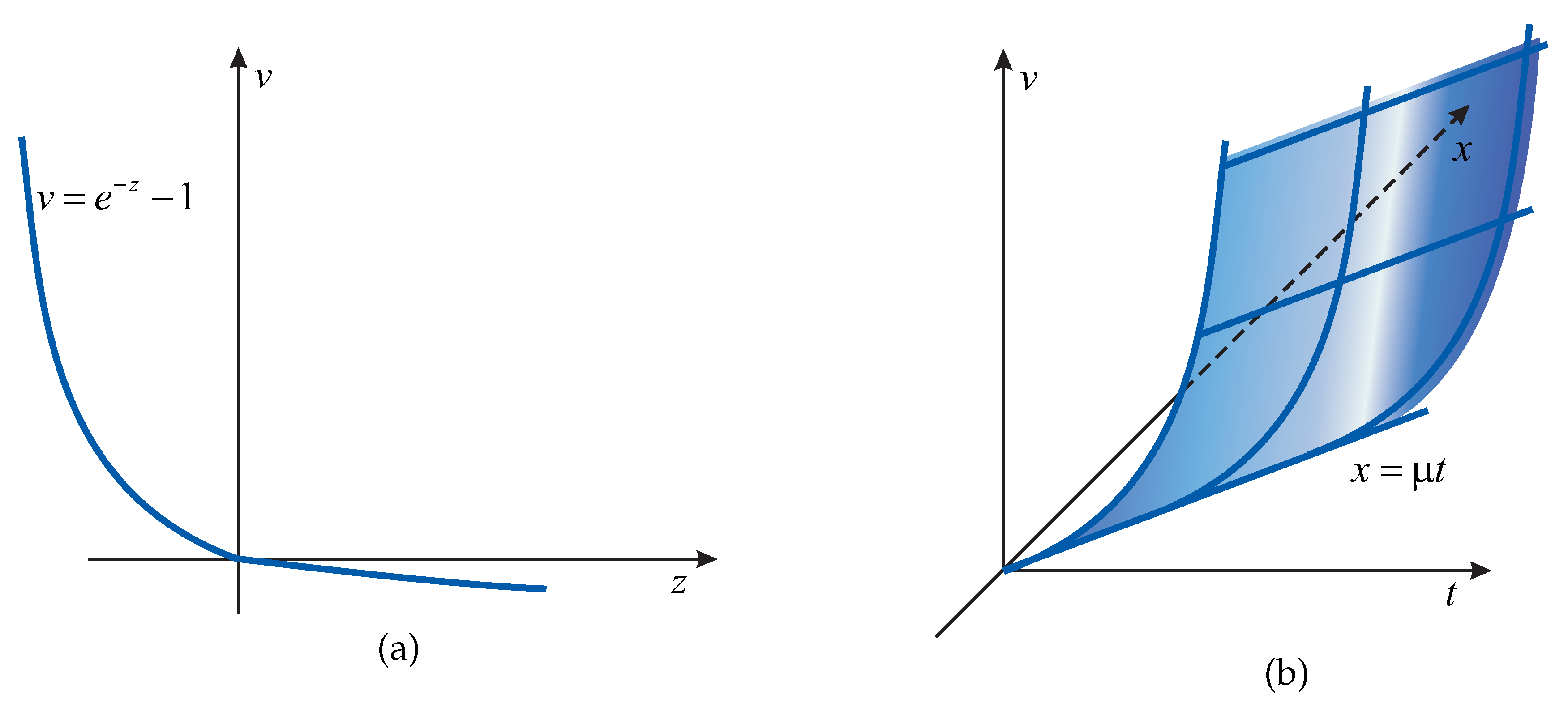
Equation (33) with separable variables is easily integrated, leading to the solution $p=-\mu \sigma +C{v}^{-1/\sigma }$. From the initial conditions, it follows that $C=0$ and therefore $v=-\mu \sigma z$; i.e., $u=-\mu \sigma (x-\mu t)$. This solution can be easily obtained without any transformations. Still, we have shown here in passing that this is the unique continuous non-trivial solution to problem (3), (4) in the considered case. Figure 1 shows the diffusion wave corresponding to this solution.

2. Consider $f(v)=1/\sigma >0$, $g(v)=\alpha v^{\beta },\alpha >0,\beta >0$, $h(v)\equiv 0$. This case corresponds to the convection–diffusion equation [9,10]. Then the problem (32) with $p\ne 0$ takes the form

$$v\frac{dp}{dv}+\frac{p}{\sigma }+\mu +\alpha v^{\beta }=0,p(0)=-\mu \sigma .$$

(34)

Let us replace the independent variable with the variable $w=\alpha v^{\beta }$. Then, since ${w|}_{v=0}=0$, problem (34) takes the form

$$\alpha \beta w\frac{dp}{dw}+\frac{p}{\sigma }+\mu +w=0,p(0)=-\mu \sigma .$$

(35)

Equation (35) is a first-order linear ODE and can also be explicitly integrated. The general solution is

$$p=-\frac{\sigma w}{\alpha \beta \sigma +1}+C{w}^{-1/\alpha \beta \sigma }-\mu \sigma .$$

The initial condition leads to $C=0$. Then, returning to the variables $v,z$, we have the Cauchy problem:

$$\frac{dv}{dz}=-\frac{\sigma \alpha v^{\beta }}{\alpha \beta \sigma +1}-\mu \sigma ,v(0)=0.$$

(36)

The solution to Equation (36) has the form

$$z=-\left(\beta +\frac{1}{\sigma \alpha }\right)\underset{0}{\overset{v}{\int }}\frac{d\zeta }{{\zeta }^{\beta }+\mu (\sigma \beta +1/\alpha )}\le 0.$$

(37)

Denote the right-hand side of (37) as $Z(v)$. Since the integrand is increasing, $Z(v)$ decreases with respect to v. This means that it is invertible, and there is $v=Z^{-1}(z)$, which is the solution to Equation (32) in the considered case. Thus, two different variants of the solution behavior are possible.

1. If $0<\beta \le 1$, then ${lim}_{v\to \infty }Z(v)=-\infty$, and the function $Z^{-1}(z)$ is defined for all $z\le 0$, and ${lim}_{z\to -\infty }{Z}^{-1}(z)=+\infty$.

2. If $\beta >1$, then the integral on the right side of (37) converges, and ${lim}_{v\to \infty }Z(v)=-Z^{\ast }$—thus, the function $Z^{-1}(z)$ is defined on the half-interval $(-Z^{\ast },0]$, and ${lim}_{z\to -Z^{\ast }}{Z}^{-1}(z)=+\infty$. Note that for non-integer $\beta$, the considered case does not satisfy the conditions of Theorem 1.

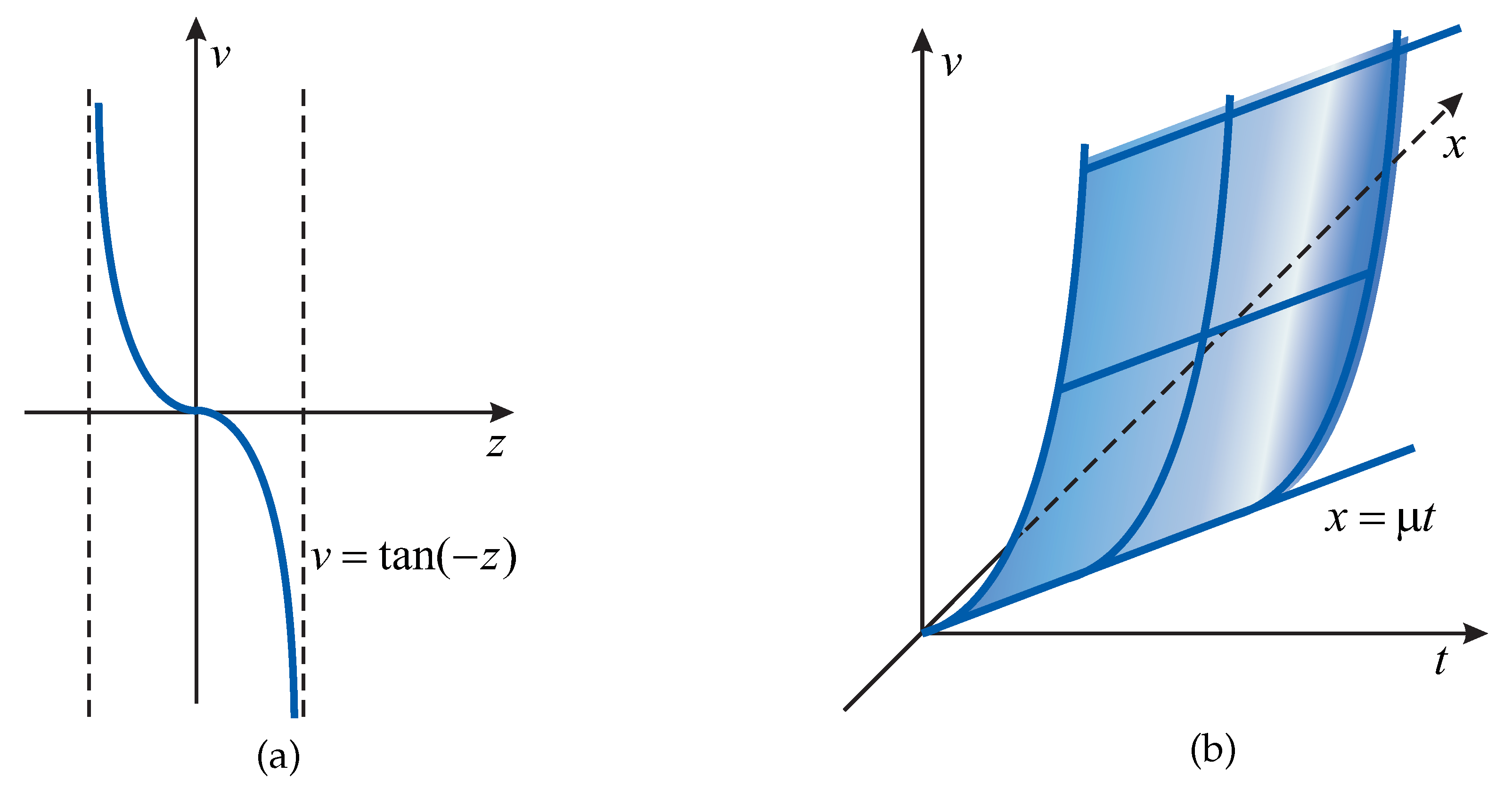
If $\beta \in \mathbb{Q}$, then the function $Z(v)$ can be obtained explicitly. For $\beta =1$ and $\beta =2$, the solutions (we denote them by $v_1^{\ast }$ and $v_2^{\ast }$) have the rather simple and descriptive form

$$v_1^{\ast }(z)=\mu \left(\sigma \beta +\frac{1}{\alpha }\right)\left[exp\left(-\frac{z\sigma \alpha }{\beta \sigma \alpha +1}\right)-1\right],$$

$$v_2^{\ast }(z)=\sqrt{\mu \left(\sigma \beta +\frac{1}{\alpha }\right)}tan\left(-z\sqrt{\frac{\mu \alpha }{\beta \sigma \alpha +1}}\right).$$

Replacing z with $x-\mu t$, we obtain the solutions $u=v_1^{\ast }(x-\mu t)$ and $u=v_2^{\ast }(x-\mu t)$ to problem (3), (4). Figure 2 and Figure 3 show the solutions $v_1^{\ast }(z)$ and $v_2^{\ast }(z)$, respectively (a), as well as corresponding diffusion waves (b).

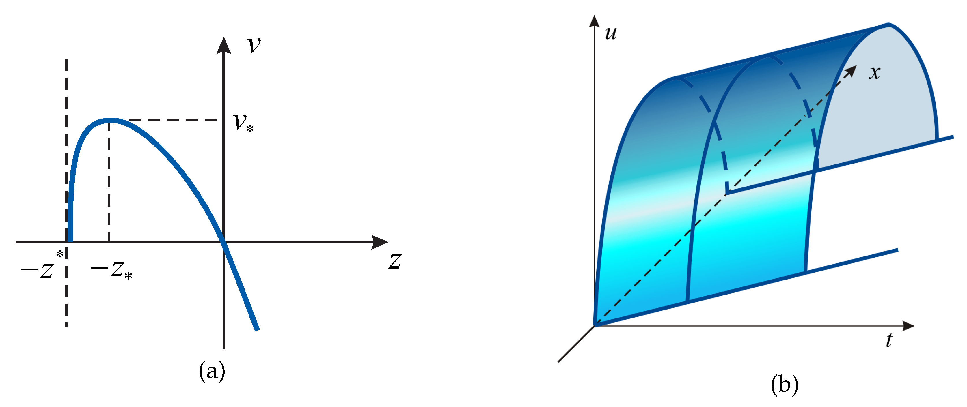
3. Finally, we consider the case where $f(v)=1/\sigma >0$, $g(v)\equiv 0$, $h(v)=\alpha v^{\beta },\alpha >0,\beta >0$, which corresponds to the generalized porous medium equation [4,8]. Then problem (32) takes the form

$$vp\frac{dp}{dv}+\frac{p^2}{\sigma }+\mu p+\alpha v^{\beta }=0,p(0)=-\mu \sigma .$$

(38)

Let us change the independent variable in Equation (38), as was performed in case 2, $w=\alpha v^{\beta }$. Then, problem (38) takes the form

$$\beta wp\frac{dp}{dw}+\frac{p^2}{\sigma }+\mu p+w=0,p(0)=-\mu \sigma .$$

(39)

Equation (39) is nonlinear and apparently cannot be explicitly integrated. Previously, we studied problem (39) using the qualitative theory of differential equations [34]. The study showed that the function $p(w)$ is increasing, and there is a point $w^{\ast }>0$ such that $p(w^{\ast })=0$, $\underset{w\to w^{\ast }-0}{lim}{p}^{\prime }(w)=+\infty$. The point can be determined numerically, since problem (39) does not have singularities on the interval $[0,w^{\ast })$. Next, we consider the problem

$$\frac{dw}{dp}=-\frac{\beta wp}{p^2/\sigma +\mu p+w}=0,w(0)=w^{\ast },$$

(40)

where w is an unknown function and p is an independent variable. The solution to problem (40) decreases on the ray $[0,+\infty )$, and $\underset{p\to +\infty }{lim}w(p)=+0.$

Returning to the variables $v,z$, we obtain the solution $v=v_{\ast }(x)$ of the following form (see Figure 4a). For the original problem, we obtain the solution $u=v_{\ast }(x-\mu t)$, which is a solitary wave or a soliton (see Figure 4b).

6. Discussion

The results obtained can be divided into two parts. The first part relates to the strictly proven propositions regarding the existence and uniqueness of solutions to the initial-boundary problem with a specified diffusion wave front. Theorem 1 generalizes previously proven statements and is a natural development of them. Although Proposition 1 concerns one particular case, it is quite non-trivial; it is based on ideas that go back to the classic example of S. V. Kovalevskaya, which, according to the letters of Karl Weierstrass, was unexpected for the mathematical community at that time [48]. Moreover, we managed to clearly separate the cases when the solution exists on the entire numerical plane, when a numerical explosion is observed and when the solution is constructed in the form of a series, but the region of its convergence consists of the single point $t=0,x=0$.

The second part of the results concerns the construction and study of exact solutions in the form of a diffusion wave. In particular cases—but the most physically meaningful cases—we have investigated the properties of solutions. Sometimes, it has been possible to bring the construction to an explicit formula. The solutions obtained also behave differently: they can exist on the entire numerical plane, tending to infinity as they move away from the wave front; however, a numerical explosion is also possible at a finite time interval. Finally, the most interesting case that takes place for the generalized porous medium equation is related to the appearance of the soliton: it moves at a constant speed without changing shape.

7. Conclusions

In summary, we note that a nonlinear second-order evolutionary parabolic equation of a reasonably general form has been considered. The questions of the existence and uniqueness and properties of solutions with the form of a diffusion wave propagating over an absolutely cold (zero) background with a finite velocity have been studied. The propositions regarding the existence and uniqueness of solutions in the analytical functions class have been proved, and an example that is analogous to the classic example of S. V. Kovalevskaya in the considered case has been constructed. Since the theorems do not allow us to investigate the properties of solutions, we have considered ansatzes that reduce solution construction to Cauchy problems for ODEs. We managed to integrate them and obtain information about the properties of solutions in particular cases that are particularly interesting for applications.

It is supposed that this paper should give rise to a whole line of research on parabolic evolution equations with singularities. In our opinion, the following studies are of the greatest interest:

• The creation of a method for the numerical solution of the considered problems, based on the use of modern computing technologies. This can be, for example, the boundary element method, which the author has been developing in recent years in collaboration with colleagues. In this case, the segments of the constructed series will be used to eliminate the singularity;
• Increasing the dimension of problems; i.e., considering cases when the desired function depends on two $x_1,x_2$ or three spatial variables $x_1,x_2,x_3$. Here, the most interesting case is when the diffusion wave front cannot be resolved with respect to one of the coordinates $x_i$ and is, for example, a cylindrical surface with a closed generatrix;
• The complication of the models considered as systems of equations can help in more accurately describing complex natural processes [23,49];
• The final stage of the research cycle should be the use of the developed model–algorithmic apparatus to solve applied problems related to the modeling of processes that occur in Lake Baikal. The lake is the largest natural reservoir of fresh water and is included in the UNESCO World Heritage List. The author lives and works close to this unique natural object and participates in scientific projects aimed at studying and saving it.

References

- Friedman, A. Partial Differential Equations of Parabolic Type; Prentice-Hall: Englewood Cliffs, NJ, USA, 1964. [Google Scholar]
- Ladyzenskaja, O.; Solonnikov, V.; Ural’ceva, N. Linear and Quasi-Linear Equations of Parabolic Type. Translations of Mathematical Monographs; American Mathematical Society: Providence, RI, USA, 1988; Volume 23. [Google Scholar]
- DiBenedetto, E. Degenerate Parabolic Equations; Springer: New York, NY, USA, 1993. [Google Scholar] [CrossRef]
- Vazquez, J. The Porous Medium Equation: Mathematical Theory; Clarendon Press: Oxford, UK, 2007. [Google Scholar] [CrossRef]
- Barenblatt, G.; Entov, V.; Ryzhik, V. Theory of Fluid Flows through Natural Rocks; Kluwer Academic Publishers: Dordrecht, The Netherlands, 1990. [Google Scholar]
- Zeldovich, Y.B.; Raizer, Y.P. Physics of Shock Waves and High-Temperature Hydrodynamic Phenomena; Dover Publications: New York, NY, USA, 2002. [Google Scholar] [CrossRef]
- Murray, J. Mathematical Biology: I. An Introduction. In Interdisciplinary Applied Mathematics, 3rd ed.; Springer: New York, NY, USA, 2002; Volume 17. [Google Scholar] [CrossRef]
- Samarskii, A.; Galaktionov, V.; Kurdyumov, S.; Mikhailov, A. Blow-Up in Quasilinear Parabolic Equations; Walter de Gruyte: Berlin, Germany, 1995. [Google Scholar] [CrossRef]
- Lu, Y.; Klingenbergm, C.; Koley, U.; Lu, X. Decay rate for degenerate convection diffusion equations in both one and several space dimensions. Acta Math. Sci. 2015, 35, 281–302. [Google Scholar] [CrossRef]
- Polyanin, A.D. Functional separable solutions of nonlinear convection-diffusion equations with variable coefficients. Commun. Nonlinear Sci. Numer. Simul. 2019, 73, 379–390. [Google Scholar] [CrossRef]
- Andreev, V.K.; Gaponenko, Y.A.; Goncharova, O.N.; Pukhnachev, V.V. Mathematical Models of Convection; Walter de Gruyte: Berlin, Germany, 2012. [Google Scholar] [CrossRef]
- Polyanin, A.D.; Zaitsev, V.F. Handbook of Nonlinear Partial Differential Equations, 2nd ed.; Chapman and Hall/CRC: New York, NY, USA, 2012. [Google Scholar] [CrossRef]
- Evans, L. Partial Differential Equations; Graduate Studies in Mathematics; American Mathematical Society: Providence, RI, USA, 2010. [Google Scholar] [CrossRef] [Green Version]
- Friedman, A. Variational Principles and Free Boundary Problems; John Wiley & Sons: New York, NY, USA, 1982. [Google Scholar]
- Sidorov, A.F. Analytic representations of solutions of nonlinear parabolic equations of time-dependent filtration type. Sov. Math. Dokl. 1985, 31, 40–44. [Google Scholar]
- Angenent, S. Solutions of the one-dimensional porous medium equation are determined by their free boundary. J. Lond. Math. Soc. 1990, 42, 339–353. [Google Scholar] [CrossRef] [Green Version]
- Filimonov, M.Y.; Korzunin, L.G.; Sidorov, A.F. Approximate methods for solving nonlinear initial boundary-value problems based on special constructions of series. Russ. J. Numer. Anal. Math. Model. 1993, 8, 101–125. [Google Scholar] [CrossRef]
- Kazakov, A.; Lempert, A. Existence and Uniqueness of the Solution of the Boundary-Value Problem for a Parabolic Equation of Unsteady Filtration. J. Appl. Mech. Tech. Phys. 2013, 54, 251–258. [Google Scholar] [CrossRef]
- Courant, R.; Hilbert, D. Methods of Mathematical Physics. Vol. II: Partial Differential Equations; Interscience Publishers, Inc.: New York, NY, USA, 2008. [Google Scholar]
- Kazakov, A.; Spevak, L. An analytical and numerical study of a nonlinear parabolic equation with degeneration for the cases of circular and spherical symmetry. Appl. Math. Model. 2016, 40, 1333–1343. [Google Scholar] [CrossRef]
- Kazakov, A.L.; Kuznetsov, P.A. On One Boundary Value Problem for a Nonlinear Heat Equation in the Case of Two Space Variables. J. Appl. Ind. Math. 2014, 8, 255–263. [Google Scholar] [CrossRef]
- Kazakov, A.L.; Kuznetsov, P.A. On the Analytic Solutions of a Special Boundary Value Problem for a Nonlinear Heat Equation in Polar Coordinates. J. Appl. Ind. Math. 2018, 812, 227–235. [Google Scholar] [CrossRef]
- Kazakov, A.; Kuznetsov, P.; Lempert, A. Analytical solutions to the singular problem for a system of nonlinear parabolic equations of the reaction-diffusion type. Symmetry 2020, 12, 999. [Google Scholar] [CrossRef]
- Brebbia, C.A.; Telles, J.C.F.; Wrobel, L.C. Boundary Element Techniques; Springer: Berlin, Germany, 1984. [Google Scholar] [CrossRef]
- Wrobel, L.; Brebbia, C. The dual reciprocity boundary element formulation for nonlinear diffusion problems. Comput. Methods Appl. Mech. Eng. 1987, 65, 147–164. [Google Scholar] [CrossRef]
- AL-Bayati, S.A.; Wrobel, L.C. A novel dual reciprocity boundary element formulation for two-dimensional transient convection-diffusion-reaction problems with variable velocity. Eng. Anal. Bound. Elem. 2018, 94, 60–68. [Google Scholar] [CrossRef]
- Kazakov, A.; Spevak, L. Numerical and analytical studies of a nonlinear parabolic equation with boundary conditions of a special form. Appl. Math. Model. 2013, 37, 6918–6928. [Google Scholar] [CrossRef]
- Kazakov, A.; Spevak, L.; Nefedova, O.; Lempert, A. On the analytical and numerical study of a two-dimensional nonlinear heat equation with a source term. Symmetry 2020, 12, 921. [Google Scholar] [CrossRef]
- Filimonov, M.Y. Application of method of special series for solution of nonlinear partial differential equations. AIP Conf. Proc. 2014, 1631, 218. [Google Scholar] [CrossRef]
- Fedotov, V.P.; Spevak, L.F. One approach to the derivation of exact integration formulae in the boundary element method. Eng. Anal. Bound. Elem. 2008, 32, 883–888. [Google Scholar] [CrossRef]
- Ovsiannikov, L.V. Group Analysis of Differential Equations; Academic Press: New York, NY, USA, 1982. [Google Scholar]
- Kazakov, A.L.; Orlov, S.S.; Orlov, S.S. Construction and study of exact solutions to a nonlinear heat equation. Sib. Math. J. 2018, 59, 427–441. [Google Scholar] [CrossRef]
- Kazakov, A.L. On exact solutions to a heat wave propagation boundary-value problem for a nonlinear heat equation. Sib. Electron. Math. Rep. 2019, 16, 1057–1068. [Google Scholar] [CrossRef]
- Kazakov, A.L. Construction and Investigation of Exact Solutions with Free Boundary to a Nonlinear Heat Equation with Source. Sib. Adv. Math. 2020, 30, 91–105. [Google Scholar] [CrossRef]
- Foias, C.; Sell, G.R.; Temam, R. Inertial manifolds for nonlinear evolutionary equations. J. Differ. Equ. 1988, 73, 309–353. [Google Scholar] [CrossRef] [Green Version]
- Constantin, P.; Foias, C.; Nicolaenko, B.; Teman, R. Integral Manifolds and Inertial Manifolds for Dissipative Partial Differential Equations; Springer: New York, NY, USA, 1989. [Google Scholar] [CrossRef]
- Cholewa, J.W.; Dlotko, T. Global Attractors in Abstract Parabolic Problems; Cambridge University Press: Cambridge, UK, 2000. [Google Scholar] [CrossRef] [Green Version]
- Gal, C.G. On a class of degenerate parabolic equations with dynamic boundary conditions. J. Differ. Equ. 2012, 253, 126–166. [Google Scholar] [CrossRef] [Green Version]
- Lee, J.; Toi, V.M. Attractors for nonclassical diffusion equations with dynamic boundary conditions. Nonlinear Anal. 2020, 195, 111737. [Google Scholar] [CrossRef]
- Antontsev, S.; Shmarev, S. Evolution PDEs with Nonstandard Growth Conditions. Existence, Uniqueness, Localization, Blow-Up; Atlantis Press: Paris, France, 2015. [Google Scholar] [CrossRef]
- Antontsev, S.; Shmarev, S. Global estimates for solutions of singular parabolic and elliptic equations with variable nonlinearity. Nonlinear Anal. Theory Methods Appl. 2020, 195, 111724. [Google Scholar] [CrossRef]
- Kosov, A.A.; Semenov, E.I. Exact solutions of the nonlinear diffusion equation. Sib. Math. J. 2019, 60, 93–107. [Google Scholar] [CrossRef]
- Stepanova, I.V. Symmetry of heat and mass transfer equations in case of dependence of thermal diffusivity coefficient either on temperature or concentration. Math. Methods Appl. Sci. 2018, 41, 3213–3226. [Google Scholar] [CrossRef]
- Stepanova, I.V. Group analysis of variable coefficients heat and mass transfer equations with power nonlinearity of thermal diffusivity. Appl. Math. Comput. 2019, 343, 57–66. [Google Scholar] [CrossRef]
- Olver, P.J. Direct reduction and differential constraints. Proc. R. Soc. Lond. 1994, 444, 509–523. [Google Scholar] [CrossRef]
- Sinelshchikov, D.I.; Kudryashov, N.A. Integrable Nonautonomous Lienard-Type Equations. Theor. Math. Phys. 2018, 196, 1230–1240. [Google Scholar] [CrossRef]
- Guha, P.; Ghose-Choudhury, A. Nonlocal transformations of the generalized Lienard type equations and dissipative Ermakov-Milne-Pinney systems. Int. J. Geom. Methods Mod. Phys. 2019, 16, 1950107. [Google Scholar] [CrossRef] [Green Version]
- Kozlov, V.V. Sofya Kovalevskaya: A mathematician and a person. Russ. Math. Surv. 2000, 55, 1175–1192. [Google Scholar] [CrossRef]
- Leont’ev, N.E. Exact solutions to the problem of deep-bed filtration with retardation of a jump in concentration within the framework of the nonlinear two-velocity model. Fluid Dyn. 2017, 52, 165–170. [Google Scholar] [CrossRef]
Figure 1.
Diffusion wave .
Figure 2.
(a) Solution and (b) the diffusion wave.
Figure 3.
Figure 4.
(a) Solution and (b) the soliton.
Publisher’s Note: MDPI stays neutral with regard to jurisdictional claims in published maps and institutional affiliations. |
© 2021 by the author. Licensee MDPI, Basel, Switzerland. This article is an open access article distributed under the terms and conditions of the Creative Commons Attribution (CC BY) license (https://creativecommons.org/licenses/by/4.0/).
Share and Cite
MDPI and ACS Style
Kazakov, A. Solutions to Nonlinear Evolutionary Parabolic Equations of the Diffusion Wave Type. Symmetry 2021, 13, 871. https://doi.org/10.3390/sym13050871
AMA Style
Kazakov A. Solutions to Nonlinear Evolutionary Parabolic Equations of the Diffusion Wave Type. Symmetry. 2021; 13(5):871. https://doi.org/10.3390/sym13050871
Chicago/Turabian StyleKazakov, Alexander. 2021. "Solutions to Nonlinear Evolutionary Parabolic Equations of the Diffusion Wave Type" Symmetry 13, no. 5: 871. https://doi.org/10.3390/sym13050871
Note that from the first issue of 2016, this journal uses article numbers instead of page numbers. See further details here.