
M-Parameterized N-Soft Topology-Based TOPSIS Approach for Multi-Attribute Decision Making


Abstract
:1. Introduction
2. Preliminaries
3. M-Parameterized N-Soft Set (MPNSS)
4. M-Parameterized N-Soft Topology
- good food quality,
- economical.
- (1)
- .
- (2)
- Arbitrary union of elements ofis a member of,i.e.,.
- (3)
- Finite intersection of elements ofis a member ofi.e.,.
- (1)
- The universal MPNSS and are MPNS-closed sets.
- (2)
- Finite MPNS-union of the MPNS-closed sets are MPNS-closed sets.
- (3)
- Arbitrary MPNS-intersection of the MPNS-closed sets are MPNS-closed sets.
- (1)
- and are MPNS-closed sets.
- (2)
- If is a given collection of MPNS-closed sets, thenis MPNS-open set. So that is a MPNS-closed set.
- (3)
- In the same way, if is MPNS-closed set for , thenis MPNS-open set. Hence, is a MPNS-closed set.
- (1)
- and are said to be equivalent MPNS-topologies, if either or .
- (2)
- If then is MPNS-finer than or is MPNS-coarser than .
- (1)
- (2)
- Let be a collection of MPNSSs in Then and , , thus and . Thus, .
- (3)
- Let Then and . Since and , thereforeConsequently, establishes MPNS topology on and is a MPNS-topological space on universal MPNSS .
- (1)
- There exists one or multiple elements β containing , for each
- (2)
- If intersection of and contains then there must exist a containing in such a way that
- (1)
- (2)
- (3)
- (4)
- .
- (1)
- Let , then if and only if . Therefore, .
- (2)
- Let . From the definition of a MPNS-interior, and . is the biggest MPNS open set that is contained by Hence, .
- (3)
- By definition of a MPNS interior, and .Then, .is the biggest MPNS open set that is contained by .Hence, . Conversely, consider and Then, and . Therefore, .
- (4)
- and .Then, .is the biggest MPNS open set that is contained by .Hence, .
- (1)
- (2)
- (1)
- Let . Then, is a MPNS closed set. Therefore, and are equal. Hence .
- (2)
- Let . By the definition of a MPNS-closure, and . is the smallest MPNS-closed set that containing . Then .
- (1)
- (2)
- (1)
- Fr=
- (2)
- =
- (3)
- is open
- (4)
- is closed
- (5)
- is both open and closed
- (1)
- (2)
5. MPNS-Topology Based MADM
| Algorithm 1: (MPNS topology based method 1). |
|
| Algorithm 2: (MPNS topology based method 2). |
|
Numerical Example
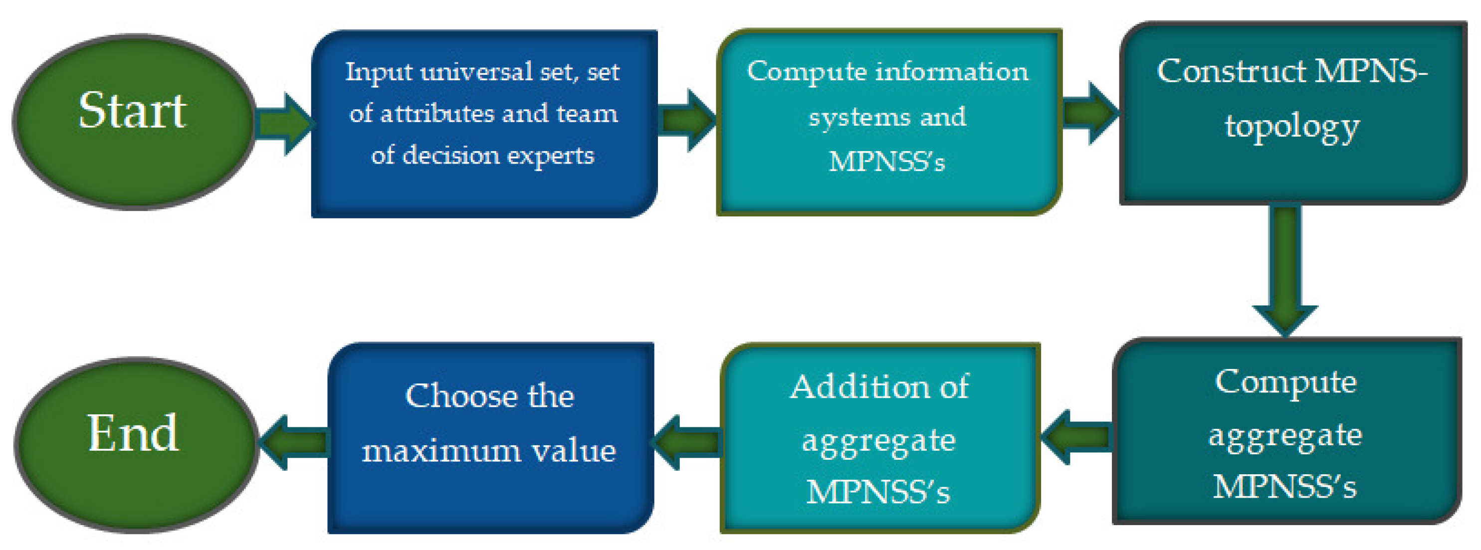
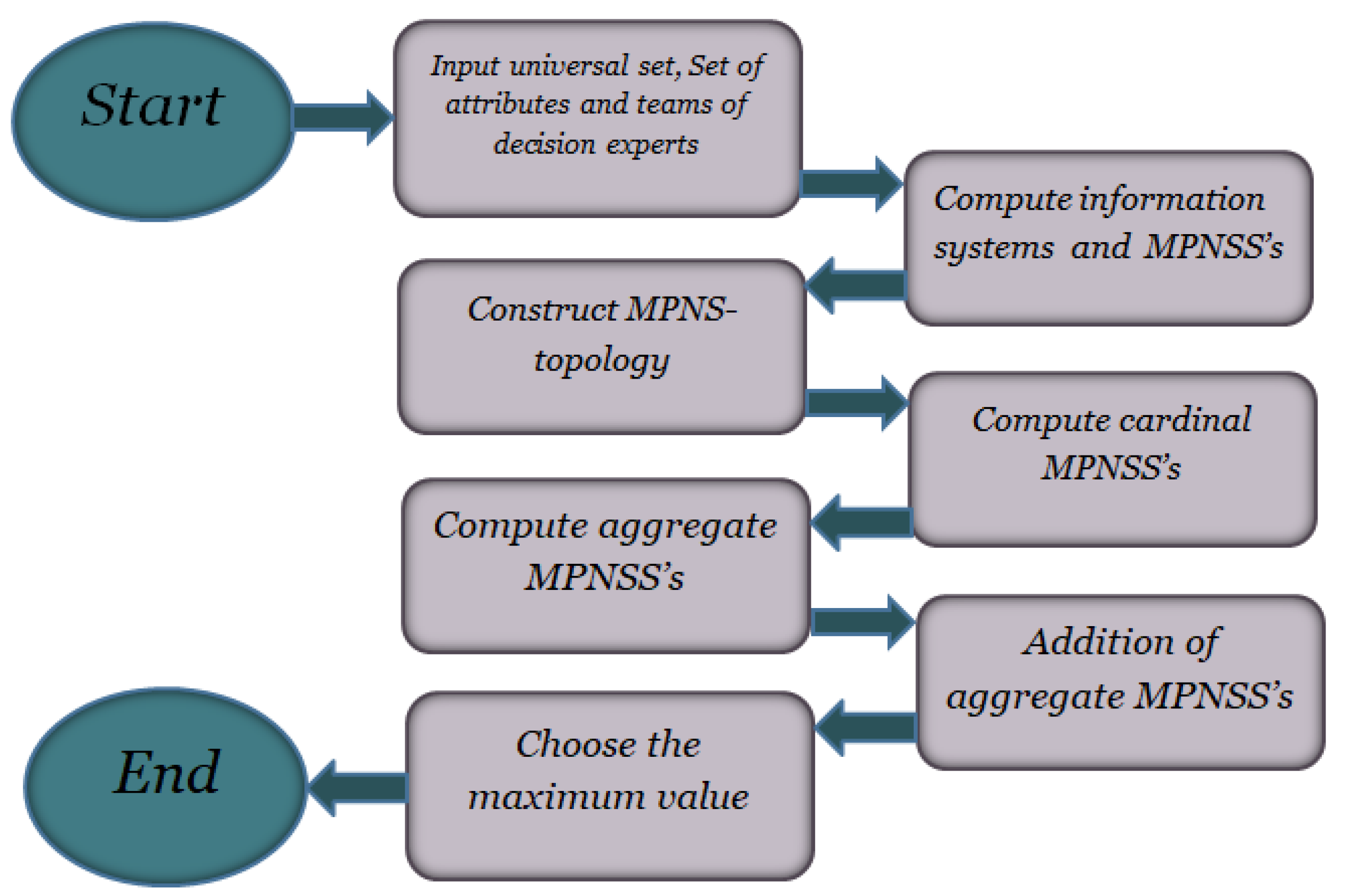
- Step 1:
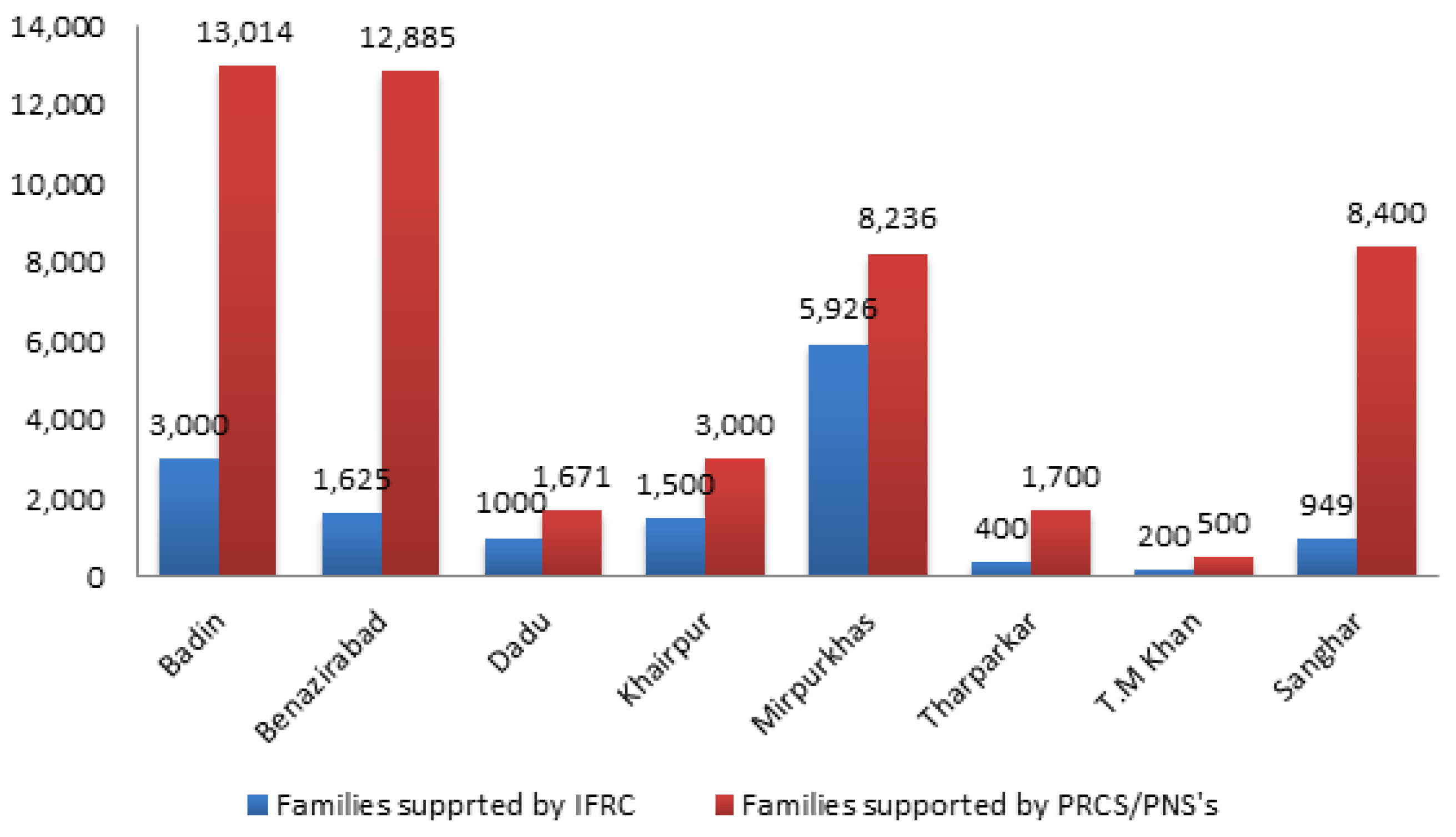
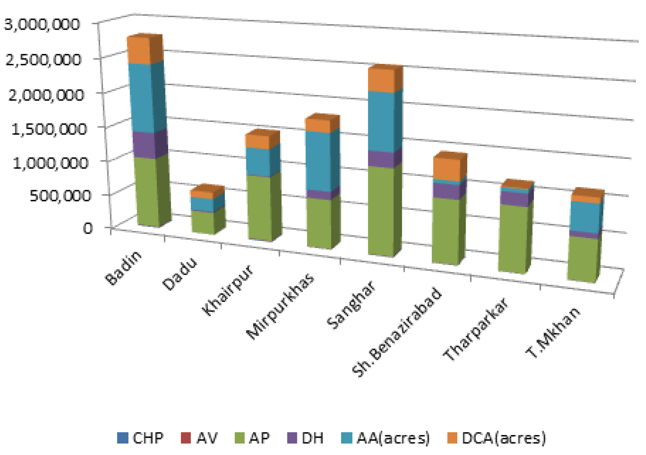
- Let be the collection of the worst affected districts of Sindh, where = Badin, = Dadu, = Khairpur, = Mirpurkhas, = Sh. Banazirabad, = Tharparkar, = Sanghar, = T. M. Khan. Let be the set of decision variables, whereThe great challenge of this problem is to get estimation of most affected area on the basis of grading assessment of decision experts in two teams, in order to distribute the resources and funding according to the damage level. Let and be two grading sets.
- Step 2:
- PRCS Sindh branch sent two rapid evaluation teams to get estimation of immediate requirements to make urgent progressive scheme in most affected district firstly. We consider two decision-makers (DMs) and made two separate teams for assessment and analysis of consequences of flood. Both teams gave the report about the situation of badly affected districts in accordance with chosen subsets by team- and team- in terms of sets, in which grades are given to the attributes. i.e., and , respectively. After a complete research both teams construct 10P10SS’s, and over First we construct a 10P10SS over namely on the assessment of other departments of different institutions, feed back of people of affected areas and according to demand of assessment teams of PRCS. The information system corresponding to collected data from other resources and people of affected areas is given in Table 10 and its matrix form is given in Table 11.
- Step 3:
- Now we construct a 10P10S-topology as
- Step 4:
- Computing aggregate 10P10SS’s of all 10P10S-open sets by using Equation (1), given by
- Step 5:
- By adding and , we obtain the final decision. There is unnecessary to incorporate the aggregate 10P10S-sets of and . By adding the aggregate 10P10SS’s, and to the sum of and , we get the same ranking. Hence there is no need to include these two sets. We haveThis shows that
- Step 6:
- By taking maximum of grading values, we obtain the optimal decision as,The greatest aggregated value is 117. This shows that = Badin is most affected district than others. PRCS, Sindh Branch responded rapidly through its district branches. Teams comprising volunteers and trained staff in emergency relief, first assistance were posted to the badly affected areas within 24 h to implement quick requirement evaluations and deliver humanitarian assistance. Now we solve the same problem by using proposed Algorithm 2. First 3 steps are same as calculated in Algorithm 1. In Algorithm 2, we proceed from step 4.
- Step 7:
- Step 8:
- Then we find out the matrix of by using Equation (3).that means, Similarly, we can find the aggregate 10P10SS for given as,that means,
- Step 9:
- Now we find the final decision 10P10SS by adding and only because there is no need to add and
- Step 10:
- The optimal decision is obtained by taking maximum of final aggregated values as,
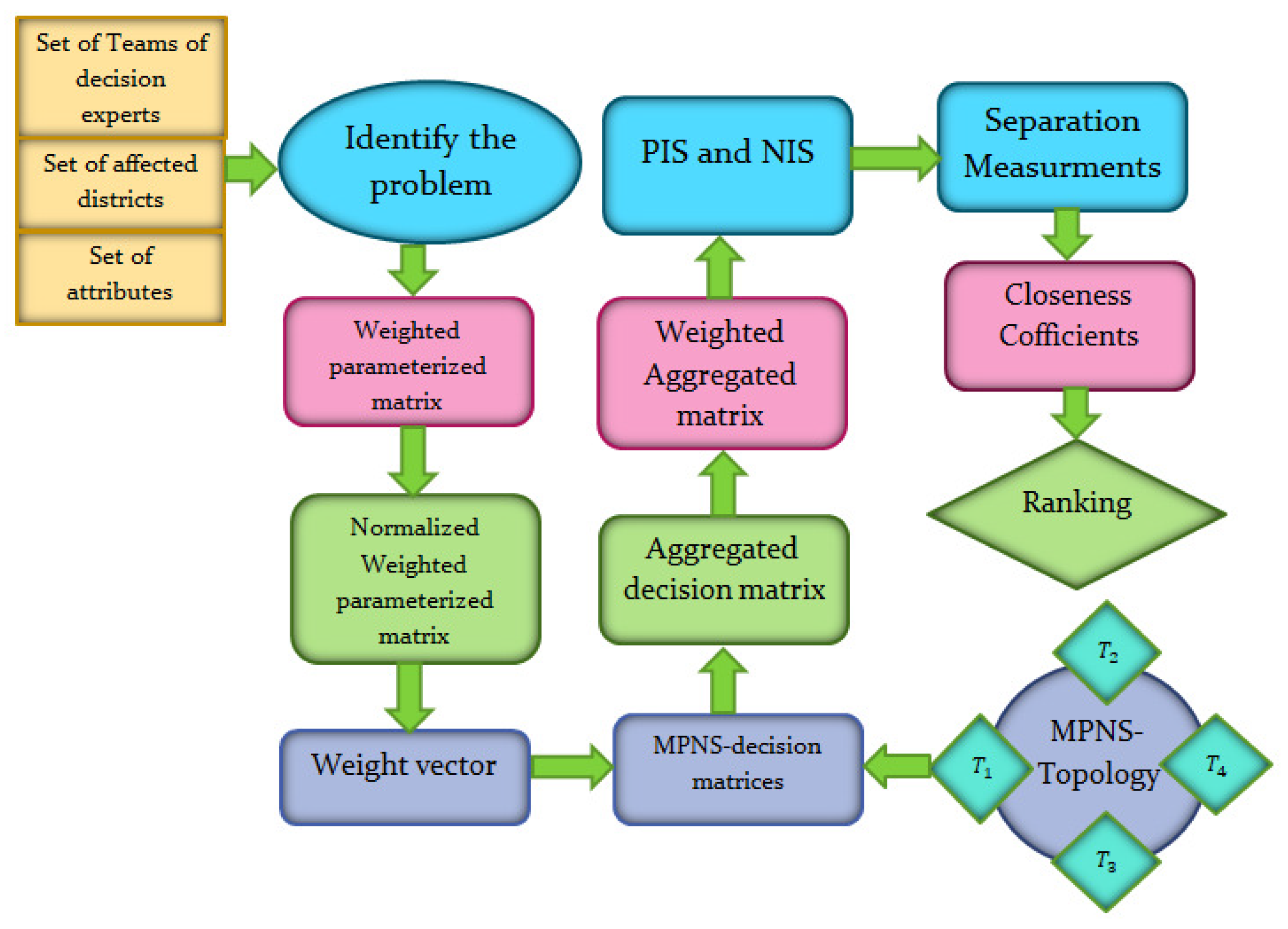
6. TOPSIS Method under M-Parameterized N-Soft Topology
- Step 1:
- Identification of decision problem:Consider is a collection of teams of decision experts, is a collection of alternatives, be two grading sets, is the set of evaluation attrbiutes.
- Step 2:
- By choosing linguistic variables from Table 16, construct weighted parameterized matrix,Decision experts assigned grades, row-wise to each parameter, represented by by using the linguistic variables. In all matrices, the first row (in bold letters) represents the grading values, assigned to parameters by chairman of PRCS according to the surveyed data of teams of other departments, by using linguistic variables from Table 17.
- Step 3:
- Creating normalized weighted parameterized matrix ,where
- Step 4:
- Creating weight vector by using the expression
- Step 5:
- Constructing MPNS-decision matrices for each team such that all make MPNS topology,Here are MPNS-elements.
- Step 6:
- The aggregated matrix can be calculated as,
- Step 7:
- Constructing the final weighted decision matrix,where
- Step 8:
- Now finding positive ideal solution (PIS) and negative ideal solution (NIS).
- Step 9:
- Calulating separation measurements and of PIS and NIS, respectively, for each parameter by making use ofand
- Step 10:
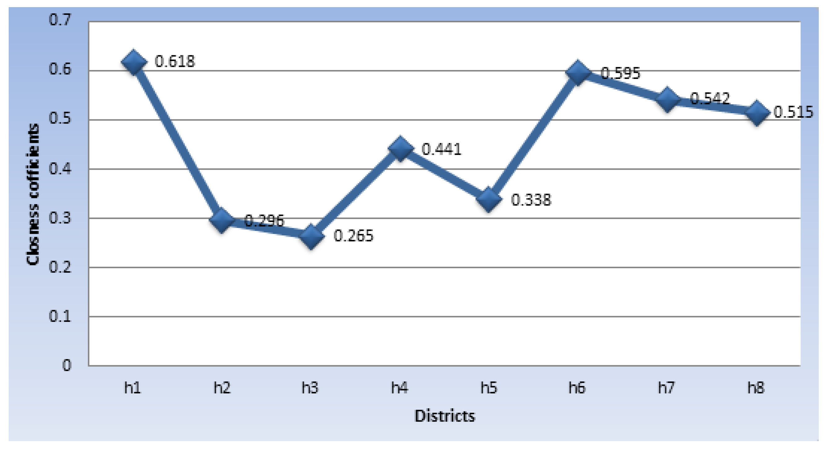
- Calculating the relative closeness,
- Step 11:
- Ranking the alternatives in descending order. The optimal choice would be the alternative with largest value of .
6.1. Numerical Example
- Step 1:
- Let is a collection of the badly affected districts of Sindh, where = Badin, = Dadu, = Khairpur, = Mirpurkhas, = Sh.Banazirabad, = Tharparkar, = Sanghar, = T.M Khan. Let be the set of evaluation attributes, whereThe major challenge is to estimate which district/area is most affected on the basis of grading values of decision experts in two teams, so as to allocate the funds accordingly to the level of damage. Let and be two grading sets.
- Step 2:
- Decision experts of assessment teams of PRCS, assigned grades to each evaluation attribute, represented by by using the linguistic variables. In all matrices, first row (in bold letters) represents the grading values, assigned to evaluation attributes by chairman of PRCS according to the information of teams of other departments, by using linguistic variables given in Table 17.
- Step 3:
- The normalized weighted parameterized matrix , by using Equation (4) is given as,
- Step 4:
- The weight vector by using Equation (5) is given as,
- Step 5:
- The 10P10S-decision matrices of two teams are given in which each row represents alternatives and each column represents evaluation attributes and all make 10P10S-topology. There is no need to write null matrix and universal matrix for 10P10S-topology.
- Step 6:
- The Aggregated matrix ¥ obtained as,
- Step 7:
- Constructing final weighted decision matrix as,
- Step 8:
- The positive ideal solution (PIS) and negative ideal solution (NIS) are given belowand
- Step 9:
- Step 10:
- The relative closeness to alternatives are given in Table 19 as follows,
- Step 11:
- The ranking order is . This shows, Badin is the most affected district.
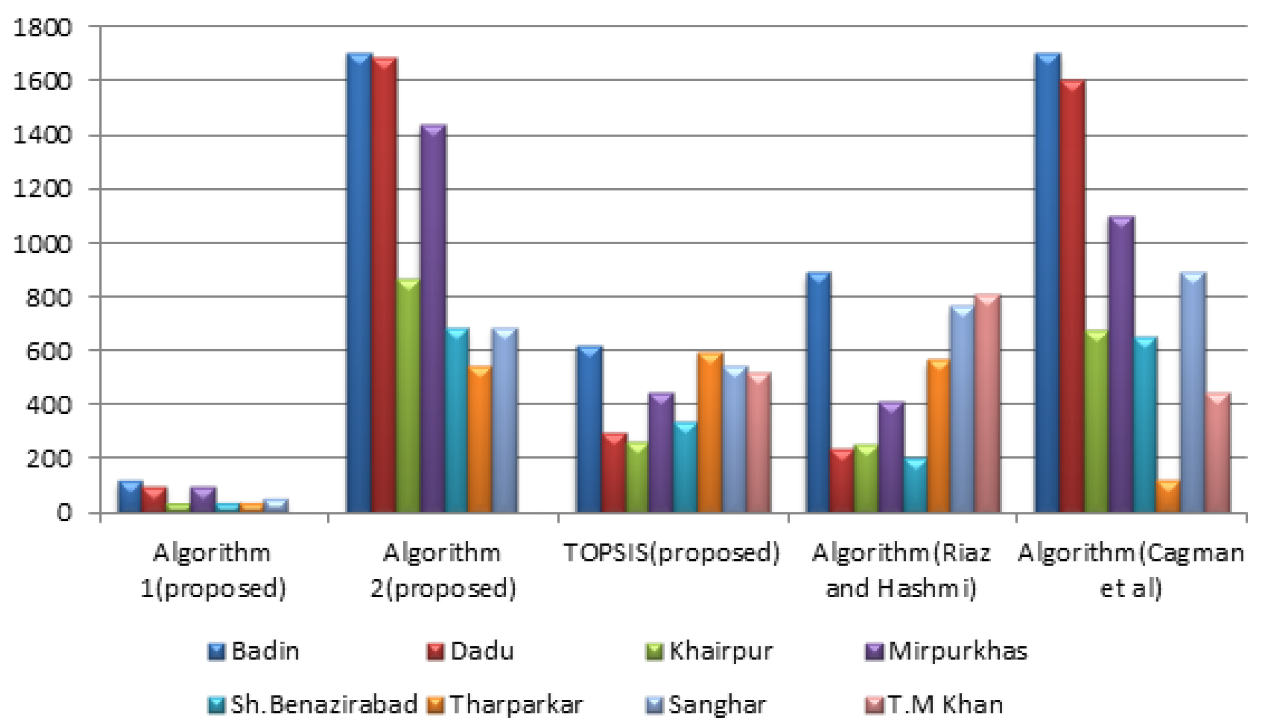
6.2. Comparison Analysis
7. Conclusions
Author Contributions
Funding
Institutional Review Board Statement
Informed Consent Statement
Data Availability Statement
Acknowledgments
Conflicts of Interest
References
- Zadeh, L.A. Information and Control. Fuzzy Sets 1965, 8, 338–353. [Google Scholar]
- Pawlak, Z. Rough sets. Int. J. Inf. Comput. Sci. 1982, 11, 341–356. [Google Scholar] [CrossRef]
- Molodtsov, D. Soft set theory-first results. Comput. Math. Appl. 1999, 37, 19–31. [Google Scholar] [CrossRef] [Green Version]
- Atanassov, K.T. Fuzzy Sets and Systems. Intuit. Fuzzy Sets 1896, 20, 87–96. [Google Scholar] [CrossRef]
- Yager, R.R. Pythagorean fuzzy subsets. In 2013 Joint IFSA World Congress and NAFIPS Annual Meeting (IFSA/NAFIPS); IEEE: New York, NY, USA, 2013; pp. 57–61. [Google Scholar]
- Yager, R.R.; Abbasov, A.M. Pythagorean membership grades, complex numbers, and decision making. Int. J. Intell. Syst. 2013, 28, 436–452. [Google Scholar] [CrossRef]
- Fatimah, F.; Rosadi, D.; Hakim, R.B.F.; Alcantud, J.C.R. N-soft sets and their decision-making algoritms. Soft Comput. 2018, 22, 3829–3842. [Google Scholar] [CrossRef]
- Riaz, M.; Çağman, N.; Zareef, I.; Aslam, M. N-Soft Topology and its Applications to Multi-Criteria Group Decision Making. J. Ournal Intell. Fuzzy Syst. 2018, 36, 6521–6536. [Google Scholar] [CrossRef]
- Akram, M.; Adeel, A.; Alcantud, J.C.R. Group decision-making methods based on hesitant N-soft sets. Expert Syst. Appl. 2019, 115, 95–105. [Google Scholar] [CrossRef]
- Akram, M.; Adeel, A.; Alcantud, J.C.R. Fuzzy N-soft sets: A novel model with applications. J. Intell. Fuzzy Syst. 2018, 35, 4757–4771. [Google Scholar] [CrossRef]
- Akram, M.; Adeel, A. TOPSIS Approach for MAGDM Based on Interval-Valued Hesitant Fuzzy N-Soft Environment. Int. J. Fuzzy Syst. 2019, 21, 993–1009. [Google Scholar] [CrossRef]
- Ashraf, S.; Abdullah, S.; Mahmood, T. Spherical fuzzy Dombi aggregation operators and their application in group decision making problems. J. Ambient. Intell. Humaniz. Comput. 2019. [Google Scholar] [CrossRef]
- Ali, M.I.; Feng, F.; Liu, X.Y.; Min, W.K.; Shabir, M. On some new operations in soft set theory. Comput. Math. Appl. 2009, 57, 1547–1553. [Google Scholar] [CrossRef] [Green Version]
- Ali, M.I. A note on soft sets, rough soft sets and fuzzy soft sets. Appl. Soft Comput. 2011, 11, 3329–3332. [Google Scholar]
- Karaaslan, F.; Hunu, F. Type-2 single-valued neutrosophic sets and their applications in multi-criteria group decision making based on TOPSIS method. J. Ambient. Intell. Humaniz. Comput. 2020. [Google Scholar] [CrossRef]
- Kumar, K.; Garg, H. TOPSIS method based on the connection number of set pair analysis under interval-valued intuitionistic fuzzy set environment. Comput. Appl. Math. 2018, 37, 1319–1329. [Google Scholar] [CrossRef]
- Maji, P.K.; Biswas, R.; Roy, A.R. Fuzzy Soft sets. J. Fuzzy Math. 2001, 9, 589–602. [Google Scholar]
- Maji, P.K.; Biswas, R.; Roy, A.R. Intuitionistic fuzzy soft sets. J. Fuzzy Math. 2001, 9, 677–691. [Google Scholar]
- Çağman, N.; Karataş, S.; Enginoglu, S. Soft topology. Comput. Math. Appl. 2011, 62, 351–358. [Google Scholar] [CrossRef] [Green Version]
- Shabir, M.; Naz, M. On soft topological spaces. Comput. Math. Appl. 2011, 61, 1786–1799. [Google Scholar] [CrossRef] [Green Version]
- Riaz, M.; Tehrim, S.T. On Bipolar Fuzzy Soft Topology with Application. Soft Comput. 2011, 24, 18259–18272. [Google Scholar] [CrossRef]
- Eraslan, S.; Karaaslan, F. A group decision making method based on TOPSIS under fuzzy soft environment. J. New Theory 2015, 3, 30–40. [Google Scholar]
- Feng, F.; Jun, Y.B.; Liu, X.; Li, L. An adjustable approach to fuzzy soft set based decision making. J. Comput. Appl. Math. 2010, 234, 10–20. [Google Scholar] [CrossRef] [Green Version]
- Feng, F.; Li, C.; Davvaz, B.; Ali, M.I. Soft sets combined with fuzzy sets and rough sets, a tentative approach. Soft Comput. 2010, 14, 899–911. [Google Scholar] [CrossRef]
- Peng, X.D.; Yang, Y. Some results for Pythagorean fuzzy sets. Int. J. Intell. Syst. 2015, 30, 1133–1160. [Google Scholar] [CrossRef]
- Peng, X.D.; Yuan, H.Y.; Yang, Y. Pythagorean fuzzy information measures and their applications. Int. J. Intell. Syst. 2017, 32, 991–1029. [Google Scholar] [CrossRef]
- Peng, X.D.; Selvachandran, G. Pythagorean fuzzy set: State of the art and future directions. Artif. Intell. Rev. 2019, 52, 1873–1927. [Google Scholar] [CrossRef]
- Peng, X.D.; Liu, L. Information measures for q-rung orthopair fuzzy sets. Int. J. Intell. Syst. 2019, 34, 1795–1834. [Google Scholar] [CrossRef]
- Zhang, X.L.; Xu, Z.S. Extension of TOPSIS to multiple criteria decision making with pythagorean fuzzy sets. Int. J. Intell. Syst. 2014, 29, 1061–1078. [Google Scholar] [CrossRef]
- Zhang, L.; Zhan, J. Fuzzy soft β-covering based fuzzy rough sets and corresponding decision-making applications. Int. J. Mach. Learn. Cybernatics 2019, 10, 1487–1502. [Google Scholar] [CrossRef]
- Zhang, L.; Zhan, J.; Alcantud, J.C.R. Novel classes of fuzzy soft β-coverings-based fuzzy rough sets with applications to multi-criteria fuzzy group decision making. Soft Comput. 2019, 23, 5327–5351. [Google Scholar] [CrossRef]
- Garg, H.; Arora, R. Generalized intuitionistic fuzzy soft power aggregation operator based on t-norm and their application in multicriteria decision-making. Int. J. Intell. Syst. 2019, 34, 215–246. [Google Scholar] [CrossRef]
- Garg, H.; Arora, R. Dual hesitant fuzzy soft aggregation operators and their application in decision-making. Cogn. Comput. 2018, 10, 769–789. [Google Scholar] [CrossRef]
- Pamucar, D.; Jankovic, A. The application of the hybrid interval rough weighted Power-Heronian operator in multi-criteria decision making. Oper. Res. Eng. Sci. Theory Appl. 2020, 3, 54–73. [Google Scholar] [CrossRef]
- Riaz, M.; Davvaz, B.; Fakhar, A.; Firdous, A. Hesitant fuzzy soft topology and its applications to multi-attribute group decision-making. Soft Comput. 2020. [Google Scholar] [CrossRef]
- Riaz, M.; Smarandache, F.; Firdous, A.; Fakhar, A. On soft rough topology with multi-attribute group decision making. Mathematics 2019, 7, 67. [Google Scholar] [CrossRef] [Green Version]
- Riaz, M.; Agman, N.; Wali, N.; Mushtaq, A. Certain properties of soft multi-set topology with applications in multi-criteria decision making. Decis. Making: Appl. Manag. Eng. 2020, 3, 70–96. [Google Scholar] [CrossRef]
- Riaz, M.; Hashmi, M.R. Linear Diophantine fuzzy set and its applications towards multi-attribute decision making problems. J. Intell. Fuzzy Syst. 2019, 37, 5417–5439. [Google Scholar] [CrossRef]
- Kamaci, H. Linear Diophantine fuzzy algebraic structures. J. Ambient. Intell. Humaniz. Comput. 2021. [Google Scholar] [CrossRef]
- Çağman, N.; Enginoglu, S.; Çitak, F. Fuzzy soft set theory and its applications. Iran. J. Fuzzy Syst. 2011, 8, 137–147. [Google Scholar]
- Tehrim, S.T.; Riaz, M. A novel extension of TOPSIS to MCGDM with bipolar neutrosophic soft topology. J. Intell. Fuzzy Syst. 2019, 37, 5531–5549. [Google Scholar] [CrossRef]


| ⋯ | ||||
|---|---|---|---|---|
| ⋯ | ||||
| ⋯ | ||||
| ⋮ | ⋮ | ⋮ | ⋮ | ⋮ |
| ⋯ |
| ◊ | ||||||||
| • | • | |||||||
| • | • | |||||||
| • | † | |||||||
| † | † | • |
| 3 | 0 | 3 | 5 | 3 | 4 | 2 | 0 | |
| 2 | 5 | 4 | 0 | 2 | 5 | 0 | 3 | |
| 5 | 4 | 0 | 2 | 1 | 2 | 3 | 2 | |
| 1 | 2 | 5 | 1 | 0 | 3 | 4 | 3 |
| 2 | 1 | 4 | 4 | 5 | 3 | 5 | 4 | |
| 1 | 0 | 3 | 2 | 3 | 4 | 1 | 5 | |
| 3 | 2 | 1 | 3 | 0 | 0 | 2 | 3 | |
| 0 | 3 | 0 | 4 | 2 | 2 | 3 | 1 |
| 5 | 5 | 5 | 0 | 5 | 5 | 5 | 5 | |
| 5 | 0 | 5 | 5 | 5 | 0 | 5 | 5 | |
| 0 | 5 | 5 | 5 | 5 | 5 | 5 | 5 | |
| 5 | 5 | 0 | 5 | 5 | 5 | 5 | 5 |
| 0 | 5 | 0 | 0 | 0 | 0 | 0 | 5 | |
| 0 | 0 | 0 | 5 | 0 | 0 | 5 | 0 | |
| 0 | 0 | 5 | 0 | 0 | 0 | 0 | 0 | |
| 0 | 0 | 0 | 0 | 5 | 0 | 0 | 0 |
| 2 | 1 | 0 | 1 | 2 | 3 | 1 | 2 | |
| 0 | 3 | 2 | 0 | 3 | 2 | 1 | 0 | |
| 0 | 2 | 3 | 2 | 3 | 1 | 0 | 2 | |
| 3 | 1 | 2 | 3 | 0 | 1 | 2 | 1 |
| 3 | 1 | 3 | 5 | 3 | 4 | 2 | 2 | |
| 2 | 5 | 4 | 0 | 3 | 5 | 1 | 3 | |
| 5 | 4 | 3 | 2 | 3 | 2 | 3 | 2 | |
| 3 | 2 | 5 | 3 | 0 | 3 | 4 | 3 |
| 2 | 0 | 0 | 1 | 2 | 3 | 1 | 0 | |
| 0 | 3 | 2 | 0 | 2 | 2 | 0 | 0 | |
| 0 | 2 | 0 | 2 | 1 | 1 | 0 | 2 | |
| 1 | 1 | 2 | 1 | 0 | 1 | 2 | 1 |
| † | † | |||
| † | ||||
| † | ||||
| † | ||||
| 5 | 4 | 5 | 3 | 3 | 6 | 6 | 5 | |
| 7 | 4 | 2 | 3 | 1 | 2 | 2 | 3 | |
| 4 | 5 | 3 | 2 | 3 | 4 | 4 | 1 | |
| 6 | 3 | 6 | 5 | 7 | 8 | 1 | 8 | |
| 7 | 6 | 5 | 6 | 5 | 5 | 3 | 4 | |
| 3 | 2 | 4 | 5 | 6 | 4 | 4 | 2 | |
| 1 | 5 | 4 | 1 | 4 | 3 | 3 | 5 | |
| 2 | 7 | 6 | 5 | 9 | 7 | 7 | 6 |
| • | ||||
| • | • | |||
| • | ||||
| • | • | • | ||
| • | • | |||
| • | • | † | ||
| • | • | • | • |
| 5 | 4 | 3 | 3 | |
| 7 | 4 | 3 | 0 | |
| 4 | 0 | 2 | 0 | |
| 5 | 0 | 5 | 5 | |
| 0 | 0 | 6 | 0 | |
| 3 | 2 | 0 | 0 | |
| 0 | 5 | 0 | 1 | |
| 0 | 0 | 0 | 0 |
| • | |||
| • | • | ||
| • | • | ||
| • | • | • | |
| • | † | • | |
| • | • | † | |
| • | • | • |
| 4 | 3 | 2 | |
| 5 | 2 | 0 | |
| 2 | 0 | 0 | |
| 0 | 0 | 3 | |
| 0 | 0 | 0 | |
| 0 | 1 | 0 | |
| 0 | 0 | 1 | |
| 0 | 0 | 0 |
| Linguistic Terms | Grading Values |
|---|---|
| Worst (W) | |
| Very Bad (VB) | 7 |
| Bad (B) | 6 |
| Intermediate (I) | |
| Safe (S) | 3 |
| Very safe (VS) | 2 |
| Completely safe (CS) |
| Linguistic Terms | Grading Values |
|---|---|
| Very Important (VI) | |
| Important (I) | |
| Medium (M) | |
| Less important (LI) | |
| Not importantt (NI) | 0 |
| 13.351 | 30.081 | 23.297 | 22.755 | 32.122 | 9.744 | 13.779 | 21.150 |
| 21.603 | 12.668 | 8.400 | 18.007 | 16.421 | 14.319 | 16.344 | 22.513 |
| 0.618 | 0.296 | 0.265 | 0.441 | 0.338 | 0.595 | 0.542 | 0.515 |
| Method | Ranking of Alternatives | Optimal Alternative |
|---|---|---|
| Algorithm 1 (Proposed) | ||
| Algorithm 2 (Proposed) | ||
| MPNS-TOPSIS (Proposed) | ||
| Algorithm (Eraslan and Karaaslan [22]) | ||
| Algorithm (Cagman et al. [40]) | ||
| Algorithm (Tehrim and Riaz [41]) |
Publisher’s Note: MDPI stays neutral with regard to jurisdictional claims in published maps and institutional affiliations. |
© 2021 by the authors. Licensee MDPI, Basel, Switzerland. This article is an open access article distributed under the terms and conditions of the Creative Commons Attribution (CC BY) license (https://creativecommons.org/licenses/by/4.0/).
Share and Cite
Riaz, M.; Razzaq, A.; Aslam, M.; Pamucar, D. M-Parameterized N-Soft Topology-Based TOPSIS Approach for Multi-Attribute Decision Making. Symmetry 2021, 13, 748. https://doi.org/10.3390/sym13050748
Riaz M, Razzaq A, Aslam M, Pamucar D. M-Parameterized N-Soft Topology-Based TOPSIS Approach for Multi-Attribute Decision Making. Symmetry. 2021; 13(5):748. https://doi.org/10.3390/sym13050748
Chicago/Turabian StyleRiaz, Muhammad, Ayesha Razzaq, Muhammad Aslam, and Dragan Pamucar. 2021. "M-Parameterized N-Soft Topology-Based TOPSIS Approach for Multi-Attribute Decision Making" Symmetry 13, no. 5: 748. https://doi.org/10.3390/sym13050748