Comparative Assessment of the Stability of AHP and FAHP Methods

Abstract

Mathematical models describing physical, technical, economic, and other processes can be used to analyze these processes and predict their results, providing that these models are stable and their results are stable relative to the model parameters used. Small changes in the values of the model parameters correspond to small changes in the results. Multicriteria decision-making models need to check the results’ stability against the models’ main components: the values of the criteria weights and the elements of the decision matrix. In this article, we study the stability of models associated with the calculation of criteria weights. For the analysis, the most commonly used models are taken—the Analytic Hierarchy Process (AHP) method and the fuzzy Analytic Hierarchy Process (FAHP) method, in which fuzzy numbers are used under conditions of data uncertainty. Both mathematically well-based methods verify the consistency of the expert evaluations. The method of statistical simulation (Monte Carlo) is the basis for studying the results’ stability. The study checks the experts’ provided evaluations’ consistency, calculates the criteria weights, and evaluates their relative errors after a slight change in the estimates of the pairwise comparisons of the criteria provided by the experts. The matrix of comparisons of the FAHP method is constructed based on the entire expert group’s assessments. It estimates the boundaries of variance in the fuzzy criteria weights. This paper estimates the stability of the criteria’ weights associated with the mathematical methods themselves and the experts’ estimates. The results are useful to study the stability of specific MCDM methods when ranking alternatives.

1. Introduction

A mathematical model makes practical sense if its results are stable concerning the model parameters. If an insignificant variation in the values of the resulting characteristics of the model corresponds to slight variations in the model parameters. Components of Multicriteria Decision-Making (MCDM) models are represented by the criteria characterizing the process under evaluation, and these criteria’ weights.

The criteria weights provide a quantitative estimation of the importance of the criteria. Given that the use of criteria weights in MCDM methods has an essential influence on the result of the evaluations and on the making of the proper decision, an investigation of the accuracy of such evaluations is interesting and important from both the theoretical and the practical point of view. This paper contains an investigation of the stability of the evaluations of the subjective weights of the criteria and the influence of data uncertainty upon the results.

Uncertainty of data may result from the evaluation of a subjective expert, the extent of the expert’s interest, ambiguity, inaccuracy of measurements, or improperly applied methods. Various approaches, such as, in particular, fuzzy set theory and the methods of mathematical statistics, Boolean logic, logistic regression, Monte Carlo simulation, Bayesian networks, and neural networks, are used to evaluate the influence of the degree of uncertainty [1].

So-called subjective weights, obtained based on peer reviews, are most frequently applied in practice [2,3,4,5,6]. For that reason, the subjective evaluation carries an uncertainty in itself. Despite the experience and competence of the expert, the evaluations provided by the same expert may vary when solving complex problems with a large number of criteria. For example, if an expert fills in the same questionnaire several times at different times, these evaluations are usually different from each other.

There are various techniques applied in the evaluation of the weight criteria. The simplest methods are based on a ranking of the criteria depending on their significance and on the direct evaluation of the weights when the sum of the evaluations is equal to one or to 100%. The use of other scales with normalization of the results is also possible. More complex subjective methods for weight evaluation, like the AHP and FAHP, use mathematical theories and verify the consistency of the expert evaluations.

There is another approach to the quantitative evaluation of the importance of the criteria. This approach evaluates the structure of the data array—the criteria values for all the alternatives [3,7,8]. Methods like this are called objective. Objective weights are applied rarely in practice, and we disregard them in this paper. A combined evaluation of the weights, which is based on the integration of subjective and objective evaluations, is also possible [9,10,11,12].

Evans [13] related the concept of sensitivity analysis in decision-making theory to the stability of an optimal solution under variation of the model parameters and the accurate evaluation of the values of such parameters. The first significant papers in the sector of sensitivity analysis were written on the basis of using the concepts of sensitivity analysis in linear programming for the development of an optimal approach that could be applied to the classical problems of decision theory [13], and on using entropy and the least squares method [14].

Zhou et al. [15] suggested a method for the calculation of the entropy weights in the situation when the evaluation of the criteria might contain uncertainties such as, for example, interval values, and when it contains both uncertainties and incompleteness, for example, with the distribution of judgements. Wolters and Mareschal suggested three types of sensitivity analysis: (1) a fixed relation between the variation of the ranking and the variations of the alternatives based on certain criteria, (2) the influence exerted by specific variations of the points/criteria of the alternative, and (3) the minimum modification of the weights necessary to provide for the alternative to take first place [16]. The analysis was focused on and developed for the preference ranking organization method for enrichment evaluation (PROMETHEE) methods. Triantaphyllou and Sánchez [17] presented the methodology for the performance of sensitivity analysis of the weights of the decision-making criteria and the alternative efficiency values for the weighted sum model (WSM), the weighted product model (WPM), and the analytic hierarchy process (AHP) methods. Evaluation of the influence exerted by uncertainty in the SAW method was performed by Podvezko [18], who evaluated the ranges of weight intervals for the process criteria, the levels of matching and stability of the expert evaluations, and the influence of uncertainty on the ranking of the matched objects. The influence of weight variation upon the final result in the SAW method was studied by Zavadskas et al. [19], and sensitivity analysis of the SAW, TOPSIS, MOORA, and PROMETHEE methods was studied by Vinogradova [20]. Memariani et al. [21] and Alinezhad [22] studied the influence of the values of the decision matrix elements upon the results of the ranking. Moghassem [23] increased and decreased the weights of all the criteria by 5, 10, 15, and 20 percent in sensitivity analysis of the TOPSIS and VIKOR methods. Hsu et al. performed sensitivity analysis of the TOPSIS method by increasing the three maximum weights by 10% and decreasing the three minimum ones by 10% [24].

Erkut and Tarimcilar [25] suggested dividing the problems of the stability of the AHP method that are to be solved into two groups. The approach of group one assumes operations over the criteria proper, by means of calculating the alternative evaluation as the sum of the alternative evaluations multiplied by the correspondent weights, based on the criteria under evaluation. The problems in group two are solved as decision-making problems under conditions of uncertainty, with the uncertainty meaning that there are a number of possible states of the nature and only one of them can be transformed into a true state. The very meaning of state probability is directly related to the meaning of the uncertainty of the problem to be solved within the framework of risk evaluation. The authors of the paper follow the first approach to the problems, solving them graphically by creating the weight space, which is represented as all the possible combinations of the weights for the purposes of tier one of the hierarchy. Consequently, separating the weight space into sets, the spatial data can be generated from the space. Any of the alternatives possesses the highest evaluation ranking in every one of the subsets [25].

In his paper, Masuda [26] studied how variations of the entire columns of the decision-making matrix might influence the values of the alternative priorities. He suggested using the sensitivity coefficient of the finite vector of the alternative priorities for each of the column vectors in the decision matrix to show how significantly the values of the finite alternative priorities vary. Warren [27] studied in more detail the theoretical aspects of the AHP method related to the evaluation scale, the determination of the vector of eigenvalues, the issue of normalization of the weights, and so on. Mimović et al. [28] suggested an integrated application of the analytic hierarchy process (AHP) and Bayesian analysis. The Bayesian formula managed to increase the input data accuracy for the analytic hierarchy process. The AHP method was used in this paper for the representation of the objectivized input data for the Bayesian formula in situations in which statistical evaluations of the probability are not possible. In the same way, Wu et al. [29], who generated pairwise comparison matrices and verified their stability, also suggested one of the methods for verification of the stability of the AHP method. The paper by Aguarón et al. shows the development of the theoretical basis for improvement of the AHP matrix inconsistency, when the Row Geometric Mean (RGM) is used as the prioritization procedure and the Geometric Consistency Index (GCI) as the inconsistency measure [30].

A number of papers with a genuine use of the MCDM model have appeared recently in which the stability of results of the methods is studied. The paper by Chen et al. [31] evaluated the stability of the multicriteria weights by studying the GIS-based MCDM model, showing the influence of the variation of the criteria weights upon the model results in the spatial dimension and graphically. The weights were determined with the help of the AHP method and were varied from their initial values within limits of 20%. This range of variation for the initial weights was applied either to all the criteria or to each criterion, as required [31]. The paper by Deepa and Swamynathan [32] facilitated an improvement in the efficiency of internet networks through increasing their throughput capacity, by suggesting a mathematical model of a clustering protocol known as AETCP (a clustering protocol based on AHP-Entropy-TOPSIS). The mobile nodes were hierarchically organized into different clusters based on certain criteria. The integrated method for evaluation of the subjective and objective weights was applied to the evaluation of the mobile nodes. Later on, ranking of the sets of nodes was performed with the purpose selecting the nodes with the largest weight as the correspondent nodes of the cluster-head [32]. The paper by Zyoud and Fuchs-Hanusch [33] address a severe problem of a water deficit in the water supply networks. The FAHP method was used to evaluate the factors influencing the loss of water. The decision was made by diagnosing the loss-of-water risk index at the level of the pipes and the areas. The Fuzzy Synthetic Evaluation Technique (FSET) was used to evaluate the water loss index at the level of the water supply system, and Ordered Weighted Averaging (OWA) was used to aggregate individual values of the index applied to each area. A Monte Carlo simulation model was used to generate the final ranking of the areas. The results of this modeling provided sufficient stability from the point of view of the ranking of the investigated areas. Xue et al. [34] suggested a method for the evaluation of stability and safety in the construction of engineering facilities for a protective tunnel under a river using the AHP-entropy weight method and the ideal point evaluation model. The paper by Kumar et al. [35] contains an evaluation of the stability of the factor model for the environmental impact risk for materials (products/services) related to pharmaceutical drugs. The model sensitivity was checked in terms of the pro rata variation of the considered risk factor with respect to other factors, varying the weight value from 0.9 to 0.1; variations of inconsistencies were also observed for other risks. Evaluation of the supplier selection stability model was suggested by Stević et. al. [36] and executed by means of varying the weight and recording the variations in the ranking of the alternatives. The weights varied in a manner that on the increase of one criterion by a conditional unit (for example, 12%), the other criterion was, naturally, decreased correspondingly in order to satisfy the condition under which the sum of the values of all the criteria remained unchanged. Continuing with the topic of the estimation of supplier model quality, Stojić et al. [37] used the WASPAS method and suggested the calculation of the coefficient α to generate the number of relative values of the alternative; the coefficient depended on the weight parameter (α lay within the limits of 0 to 1, with increments of 0.1).

The generation of individual values of the criteria weights in the SWARA method was suggested by Zavadskas et al. [38]. The paper by Pamucar et al. [39] also evaluated the influence of the criteria (and the sub-criteria) upon the order of ranking of the alternatives, which were represented by suppliers, within the framework of the problem of increasing the service quality of third-party logistics providers. To process uncertain data under the procedure of group decision-making, the paper considered interval rough numbers (IRN) and the IRN-BWM (best worst method). The stability of the ranking of alternatives that was obtained was checked by varying the values of the coefficients of the linear combination and by the application of the operational competitiveness rankings analysis (OCRA) method [40]. Sensitivity analysis has also been used to confirm the stability of the final rankings of the results [41,42], or to verify and evaluate the feasibility of the optimal alternative [43], as well as to study the influence of the variation of the parameters and criteria weights upon the final results of ranking of the alternatives [44].

The stochastic approach to determining the uncertainty of the AHP weights has been used in different ways. Janssen [45] studied the sensitivity of the ranking of the alternatives using the effects table and compared this with the maximum evaluation of the decision-making person. The sensitivities of the rankings of alternatives to overall uncertainty in scores and priorities were analyzed using a Monte Carlo approach. Eskandari and Rabelo [46] followed another stochastic approach, and this gave these authors the opportunity to calculate the AHP weight dispersions, and to process their uncertain behavior with the help of a Monte Carlo simulation. An approach that applied fuzzy logic, an analytic hierarchy process, and a Monte Carlo simulation was used to solve the problem of the over-expenditure of funds within the framework of urban transit projects, to facilitate the effective planning of the future budget by the decision-making persons [47].

The stability of models related to calculations of subjective criteria weights is investigated in this paper. The most frequently used methods in the MCDM model—the analytic hierarchy process (AHP) method and the FAHP method, when fuzzy numbers are used under the conditions of data uncertainty—are taken for the analysis. The method of statistical simulation (Monte Carlo) is used in order to investigate the stability issues. The practical realization of the algorithm is written in the Python programming language. This paper’s results can be used as an integral part of the study of the stability of MCDM methods in the ranking of alternatives.

2. Materials and Methods

2.1. Analytic Hierarchy Process (AHP) Method

The AHP method is the most frequently used in practice among all the subjective methods for the evaluation of criteria weights. The reason is that this method is mathematically substantiated, logically understandable, and allows the performance of a quantitative determination of the consistency of the evaluations provided by each of the experts. The experts compare all the possible pairs of criteria with each other. The pairwise comparison matrix $P=\left(p_{ij}\right)$ is theoretically a ratio of unknown criteria weights: $p_{ij}=\frac{w_i}{w_j}$, (i, j = 1, 2, …, m), $p_{ij}=\frac{1}{p_{ji}}$, $p_{ii}=1$, where $m$ is the number of criteria. The element $p_{ij}$ shows by how many times the i-th criterion is more important than the j-th one. The scale 1-3-5-7-9 suggested by the author of the method—Saaty [2]—is applied to the evaluation.

The criteria weights $\overline{\omega }$ are the normalized values of the eigenvector of the matrix $P$, corresponding to the largest eigenvalue ${\lambda }_{max}$ of the matrix:

$$P\overline{\omega }=\mathsf{\lambda }\overline{\omega }$$

(1)

The degree of consistency (internal consistency) of the expert evaluations determines the Consistency Index $CI$ and the Consistency Ratio $CR$:

$$CI=\frac{{\lambda }_{max}-m}{m-1},$$

(2)

$$CR=\frac{CI}{RI},$$

(3)

where $RI$ is the average evaluation of the $CI$ of the simulated matrices of the order of m [2]. The evaluations are considered to be consistent if the Consistency Ratio is such that $CR<0.1$.

2.2. Fuzzy Analytic Hierarchy Process (FAHP) Method

In the case of weight calculations using the FAHP method, the experts evaluate the criteria using interval values. Therefore, the uncertainty is included in the evaluations themselves. Unlike the deterministic AHP case, each evaluation for triangular fuzzy numbers can be represented as (L, M, U). The most probable evaluation M corresponds to the evaluation provided by the AHP method. The number L shows the lowest possible boundary of the evaluation, and the number U the corresponding upper boundary [48].

The matrix $\tilde{P}$ for the pairwise comparison of the criteria by the expert (or total evaluation by the entire group of experts) has the following representation:

$$\tilde{P}=\left({\tilde{p}}_{ij}\right)=\left(L_{ij},M_{ij},U_{ij}\right) =\left(\begin{array}{cccc}\left(1,1,1\right)& (L_{12},M_{12},U_{12})& \dots & (L_{1m},M_{1m},U_{1m})\\ (1/U_{12},1/M_{12},1/L_{12})& \left(1,1,1\right)& \dots & (L_{2m},M_{2m},U_{2m})\\ ⋮& ⋮& ⋮& ⋮\\ (1/U_{1m},1/M_{1m},1/L_{1m})& (1/U_{2m},1/M_{2m},1/L_{2m})& \dots & \left(1,1,1\right)\end{array}\right).$$

(4)

The symmetric fuzzy numbers with respect to the main diagonal are ${\tilde{p}}_{ji}$=${\tilde{p}}_{ij}{}^{-1}=\left(\frac{1}{U_{ij}},\frac{1}{M_{ij}},\frac{1}{L_{ij}}\right)$; the main diagonal elements are ${\tilde{p}}_{ii}= \left(1,1,1\right)$.

The Chang algorithm [49] is used for calculation of the criteria weights. The value ${\tilde{S}}_i,$ called the extension of the fuzzy synthesis, is calculated for the i-th criterion using the following formula:

$${\tilde{S}}_i={\displaystyle \sum }_{j=1}^{\mathrm{m}}{\tilde{p}}_{ij}\otimes {\left\{{\displaystyle \sum }_{i=1}^{\mathrm{m}}{\displaystyle \sum }_{j=1}^{\mathrm{m}}{\tilde{p}}_{ij}\right\}}^{-1}; i=1,\dots ,m$$

(5)

All the criteria are compared pairwise using the value ${\tilde{S}}_i$:

$$V\left({\tilde{S}}_j\ge {\tilde{S}}_i\right)=\{\begin{array}{c}1, if M_j\ge M_i\\ \frac{L_i-U_j}{\left(M_j-U_j\right)-\left(M_i-L_i\right)}, if L_i\le U_j\\ 0, in other cases\end{array},i =1,\dots ,m; j=1,\dots ,m$$

(6)

The theory of the fuzzy numbers comparison is applied to the comparison of the values:

$$V_j=V\left({\tilde{S}}_j\ge {\tilde{S}}_1,{\tilde{S}}_2,\dots .{\tilde{S}}_{j-1},{\tilde{S}}_{j+1}, \dots ,{\tilde{S}}_m\right)=\underset{i\in \left\{1,\dots ,m;i\ne j\right\}}{\min }V\left({\tilde{S}}_j\ge {\tilde{S}}_i\right), i=1,\dots ,m.$$

(7)

The weight vector $w_j$ of the criteria is calculated using the following formula:

$$w_j=\frac{V_j}{{\sum }_{j=1}^m{V}_j}, j=1,\dots ,m.$$

(8)

3. Stability Check for the AHP and FAHP Methods

The AHP and FAHP methods are applied in Multicriteria Decision-Making (MCDM) evaluations in order to determine the criteria weights. The AHP method is applied in the deterministic case when the significance (weight) of each of the criteria is determined with one number. In this case, each expert determines the criterion significance in the matrix of pairwise comparisons of the criteria with one number (taken from the Saaty scale: 1-3-5-7-9). The FAHP method is used in conditions of data uncertainty when interval fuzzy evaluations are used for the calculations. In this case, evaluations of the pairwise comparison of the criteria (that is, the values of the FAHP method matrix) are also represented by interval fuzzy numbers.

The criteria weights can be used in the MCDM model methods if the weight evaluation methods, that is, the AHP and FAHP methods, are stable (resistant) in relation to natural random variations of the evaluations. Considering that the value M of a triangular fuzzy number is matched with the most probabilistic evaluation of the AHP method, it would be of interest to perform a parallel investigation of stability for the AHP and FAHP methods. The references suggest more than 25 scales that can be used in order to form the triangular values of the triangular fuzzy numbers. The frequently applied symmetric and asymmetric scales of triangular fuzzy numbers are used in this paper.

The stability of the AHP method can be understood in two ways: the stability of just the method, which depends upon the essence of the method or its mathematical basis, and the stability of the results, that is, the values of the criteria weights depending upon the evaluations provided by the experts that vary due to the uncertainty inherent to their thinking processes.

Both stability options are studied in this paper.

3.1. Stability Check Algorithm for the AHP Method

The quantitative evaluation of the stability and the criterion for evaluating the stability depend upon the specific problem to be solved. Thus, for the evaluation of the stabilities of the method for the MCDM model, we can apply the percentage of loss as the best alternative to the leading position, the maximum inconsistencies of the evaluations of the method, the percentage of variation of the order for the ranking of the alternatives, etc. [20].

The stability $\delta$ is evaluated in this paper as the maximum relative error of the criteria weights:

$$\delta =\underset{1\le j\le m;1\le \mathsf{\xi }\le \mathrm{T}}{\max } \frac{\left|{\omega }_j^{\left(\xi \right)}-{\omega }_j\right|}{{\omega }_j},$$

(9)

where ${\omega }_j$ is the weight of the j-th criterion, ${\omega }_j^{\left(\xi \right)}$ is the weight of the j-th criterion obtained as the result of the simulation, ξ is the simulation number, $1\le \xi \le T$, and $T$ is the number of simulations.

The stability of the AHP method itself is understood as follows.

The Saaty scale for the AHP method applies only integer evaluation numbers $p_{ij}$ from 1 to 9, showing by how many times one (the i-th) criterion is more important than the other (the j-th). With respect to the main diagonal, the symmetric evaluations are 1/$p_{ij}$—where numbers that are less than 1 show by how many times the second (j-th) criterion is less important than the first (i-th) one. To check the stability of the AHP method itself, we expand the evaluation scale and assume that any real numbers can act as evaluations. That would allow variation in a random manner of the evaluations provided by each of the experts, using the method of statistical simulation (Monte Carlo) to simulate the evaluations within the limits of certain intervals, performing a consistency check of the evaluations each time, and recording the weight variation intervals. The statistical modeling method (Monte Carlo) allows reproducing a real situation on a computer many times. This cannot be replicated in practice, or implementation may require significant resources and time.

Why did Saaty suggest an integer number scale and not expand the scale to the set of real numbers? In the latter case, it would be sufficient to compare the importance of one criterion only (for example, the most important one) in relation to all the other criteria, that is, to fill in one column (or row) only. It would then immediately be possible to fill in all the remaining rows (or columns) of the matrix. The elements would be pro rata with the elements of the one filled-in column.

Considering that the criteria weights are related to the eigenvector of the comparison matrix, it is important to determine how small variations of the matrix elements affect the values of the eigenvector elements and, correspondingly, influence the values of the criteria weights—the normalized values of the eigenvector.

The stability check algorithm for the AHP method can be represented in the following manner.

Step 1. The matrix ${\mathrm{P}}^{\left(k\right)}$ for pairwise comparison of the criteria of one of the experts (k = 1) is selected. The consistency of the evaluations ($CR<0.1$) is verified. The criteria weights Ω = (${\omega }_j$), j = 1, 2, …, m are calculated.

Step 2. The percentage q of inconsistency ${\widehat{p}}_{ij}^{\left(k\right)}$ of all the elements $p_{ij}^{\left(k\right)}$ ($i\ne j)$ with the expert evaluations (q = 5%, q = 10%) is determined. Therefore, the random simulated values of the evaluations $p_{ij}^{\left(k\right)}$ vary within the following interval ${\widehat{p}}_{ij}^{\left(k\right)}$ ∊ [$p_{ij}^{\left(k\right)}$ –$p_{ij}^{\left(k\right)}\frac{q}{100}, p_{ij}^{\left(k\right)}$ + $p_{ij}^{\left(k\right)}\frac{q}{100}]$. The elements of the main diagonal remain unchanged: $p_{ii}^{\left(k\right)}=1$.

We vary the values of the integer numbers only (the evaluations) $p_{ij}^{\left(k\right)}$ = 1, 2, …, 9 on both sides of the main diagonal. With respect to the main diagonal the symmetric elements are $p_{ji}^{\left(k\right)}=\frac{1}{p_{ij}^{\left(k\right)}}$.

Step 3. A sequence of random numbers ${\xi }_r$ (r = 1) uniformly distributed within the interval [0, 1] is selected using the method of statistical simulation (Monte Carlo). The random evaluation ${\widehat{p}}_{ij}^{\left(k\right)}$ by the k-th expert with the q-th inconsistency is calculated; this belongs to the interval [$p_{ij}^{\left(k\right)}$ –$p_{ij}^{\left(k\right)}\frac{q}{100},p_{ij}^{\left(k\right)}$ + $p_{ij}^{\left(k\right)}\frac{q}{100}]:$ ${\widehat{p}}_{ij}^{\left(k\right)}= p_{ij}^{\left(k\right)}$ – $p_{ij}^{\left(k\right)}\frac{q}{100} + 2p_{ij}^{\left(k\right)}\frac{q}{100}{\xi }_r \in$ [$p_{ij}^{\left(k\right)}$ – $p_{ij}^{\left(k\right)}\frac{q}{100},p_{ij}^{\left(k\right)}$ + $p_{ij}^{\left(k\right)}\frac{q}{100}]$.

A new random number from the sequence ${\xi }_r$ is used for each element $p_{ij}^{\left(k\right)}$ of the matrix.

Step 4. A random pairwise comparison matrix $P$ is formed from the simulated elements $P$ = $\parallel {\widehat{p}}_{ij}^{\left(k\right)}\parallel$. The consistency of the evaluations ($CR<0.1$) is verified. If the value of the consistency ratio for the evaluations is $CR\ge 0.1$, the matrix is discarded. The criteria weights Ω = (${\omega }_j^{\left(r\right)}$), (r = 1) are calculated.

Step 5. New sequences of random numbers ${\xi }_r$ ($r=2, 3,\dots ,T$) are selected, where T is the number of repetitions (simulations). Steps 3 and 4 are repeated. The criteria weights (${\omega }_j^{\left(r\right)}$), ($r=2, 3,\dots ,T$) are calculated.

Step 6. The largest values of the relative errors of the criteria weights for every j-th criterion of the AHP method are calculated for every simulation ξ: ${\delta }_j^{\left(\xi \right)}$ =$\frac{\left|{\omega }_j^{\left(\xi \right)}-{\omega }_j\right|}{{\omega }_j}$.

Step 7. The largest values of the relative errors ${\delta }_j^{\left(\xi \right)}$ of the criterion weight values for all the criteria are calculated for every simulation ξ: ${\delta }^{\xi }= \underset{j}{\max }{\delta }_j^{\left(\xi \right)}$.

Step 8. The largest value of the relative errors ${\delta }^{\xi }$ of the criteria weights for all the simulations ξ is taken as the AHP method error for the given matrix of comparison: δ = $\underset{\xi }{\max }{\delta }^{\xi }$.

3.2. Stability Check Algorithm for the AHP Method Related to the Evaluations of the Experts

The stability of the results—the values of the criteria weights depending upon the psychological state of the experts and the incomplete certainty of their evaluations—is understood as follows.

We have repeatedly proved that one and the same expert provides ambiguous evaluations when performing comparative evaluations of the importance of the same criteria, and even when ranking their importance at different moments in time. Naturally, the logic of the expert’s thinking process is not undergoing major changes at that time, and the evaluations provided by the expert do not differ significantly.

Therefore, we vary the evaluations provided by the experts using, naturally, the Saaty scale, varying their values by 1 (or 2), both towards an increase and towards a decrease of the values, while the comparative evaluations of the other criteria are also varied. However, internal inconsistency of the evaluations must not occur: the Consistency Ratio CR must be less than 0.1.

The stability check algorithm for the AHP method depending on the state and psychological condition of the experts can be represented in the following manner.

Step 1. The matrix $P^{\left(k\right)}$ for the pairwise comparison of the criteria of one of the experts (k = 1) is selected. Consistency of the evaluations ($CR<0.1$) is verified. The criteria weights Ω = (${\omega }_j$) are calculated, j = 1, 2, …, m.

Step 2. A sequence of random numbers ${\xi }_r$ (r = 1) uniformly distributed within the interval of [0, 1] is selected using the statistical simulation method (Monte Carlo). The values of all the evaluations of the experts—the elements $p_{ij}^{\left(k\right)}$ ($i\ne j)$ of the matrix $P^{\left(k\right)}—$are varied (increased or decreased) by 1. To do that, if $0\le {\xi }_r$ <0.5, the value increases. In the other case ($0.5< {\xi }_r$ ≤1), the value decreases. In order to attain complete symmetry, we exclude the value of ${\xi }_r$ = 0.5, that is, we do not vary the elements of the matrix. The two options have equal probability. If $p_{ij}^{\left(k\right)}$ = 1, the value is always increased. If $p_{ij}^{\left(k\right)}$ = 9, the value is decreased. The elements of the main diagonal remain unchanged: $p_{ii}^{\left(k\right)}=1$. The symmetric elements with respect to the main diagonal are $p_{ji}^{\left(k\right)}=\frac{1}{p_{ij}^{\left(k\right)}}$. A new random number from the sequence ${\xi }_r$ is used for each element $p_{ij}^{\left(k\right)}$ of the matrix.

Step 3. A random pairwise comparison matrix $P$ is formed of the simulated elements $P$ = $\parallel {\widehat{p}}_{ij}^{\left(k\right)}\parallel$. Consistency of evaluations ($CR<0.1$) is verified. If the value of the Consistency Ratio is $CR\ge 0.1$, the matrix is discarded. The criteria weights are calculated Ω = (${\omega }_j^{\left(r\right)}$), (r = 1).

Step 4. New sequences of random numbers ${\xi }_r$ (r = 2, 3, …, T), are selected, where T is the number of repetitions (simulations). Steps 2 and 3 are repeated. The criteria weights (${\omega }_j^{\left(r\right)}$), (r = 2, 3, …, T) are calculated.

Step 5. The relative errors of the values of the weight for each of the j-th criterion of the AHP method are calculated for every simulation ξ: ${\delta }_j^{\left(\xi \right)}$ = $\frac{\left|{\omega }_j^{\left(\xi \right)}-{\omega }_j\right|}{{\omega }_j}$.

Step 6. The largest values of the relative errors ${\delta }_j^{\left(\xi \right)}$ of the criteria weights for all the criteria are calculated for every simulation ξ: ${\delta }^{\xi }= \underset{j}{\max }{\delta }_j^{\left(\xi \right)}$.

Step 7. We take the largest value of the relative errors ${\delta }^{\xi }$ of the criteria weights over all the simulations ξ as the AHP method error for the given matrix of comparison: δ = $\underset{\xi }{\max }{\delta }^{\xi }$.

3.3. Stability Check Algorithm for the FAHP Method

Various types of uncertainties influence the evaluation of the stability of the FAHP method. As in the deterministic case, the values of the elements of the criteria comparison matrix depend on the logic of the thinking of the experts, and their state at the moment of evaluation. Besides, the fuzzy method itself includes uncertainty in the evaluations—a triad of values is used instead of a one-point evaluation. It should also be kept in mind that the stability evaluation for the FAHP method refers solely to the weight evaluation algorithm used by us (4)–(8).

The stability check for the FAHP method for the calculation of the criteria weights can be represented in the form of the following steps.

Step 1. A fuzzy pairwise comparison matrix for the criteria is formed on the basis of the AHP matrix $M=\left(M_{ij}\right)$: $\tilde{P}=\left({\tilde{p}}_{ij}\right)=\left(L_{ij},M_{ij},U_{ij}\right)$. The values $L_{ij}$ and $U_{ij}$ vary depending on the selected symmetric or asymmetric scale of the fuzzy number.

Step 2. The consistency of evaluations ($CR<0.1$) of the matrix M $=\left(M_{ij}\right)$ is verified. If the Consistency Ratio is $CR\ge 0.1$, the pairwise comparison matrix is discarded.

Step 3. A sequence of random numbers ${\xi }_r$ ($r=1$), uniformly distributed within the interval of [0, 1], is selected using the statistical simulation method (Monte Carlo). The values of all the $M_{ij}$ evaluations of the experts – the elements $\left({\tilde{p}}_{ij}\right)=\left(L_{ij},M_{ij},U_{ij}\right)$ ($i\ne j)$ of the matrix $\tilde{P}$—are varied (increased or decreased) by 1. To do that, if $0\le {\xi }_r$ <0.5, the value increases. In the other case ($0.5< {\xi }_r$ ≤1), the value decreases. In order to attain complete symmetry, we exclude the value of ${\xi }_r$ = 0.5, that is, we do not vary the elements of the matrix. The two options have equal probability. If at least one of the numbers $\left(L_{ij},M_{ij},U_{ij}\right)$ is equal to 1, the value is always increased. If at least one of the numbers $\left(L_{ij},M_{ij},U_{ij}\right)$ is equal to 9, the value is decreased. The elements of the main diagonal remain unchanged: $\left({\tilde{p}}_{ii}\right)=\left(L_{ii},M_{ii},U_{ii}\right)=\left(1, 1, 1\right)$. The symmetric elements with respect to the main diagonal are $\left({\tilde{p}}_{ii}\right)=\left(L_{ii}, M_{ii}, U_{ii}\right)=\left(\frac{1}{{\tilde{p}}_{ii}}\right)=\left(\frac{1}{U_{ii}},\frac{1}{M_{ii}},\frac{1}{L_{ii}}\right)$. A new random number from the sequence ${\xi }_r$ is used for each element ${\tilde{p}}_{ij}$ of the matrix.

The matrix $\tilde{P}$ is formed from the values of the matrix M $=\left(M_{ij}\right)$. The consistency of evaluation of the values of the matrix M ($CR<0.1$) is verified. If the Consistency Ratio is $CR\ge 0.1$, the pairwise comparison matrix is discarded and a new fuzzy matrix $\tilde{P}$ is formed.

The criteria weights $\left(\Omega ={\omega }_j^{\left(r\right)}\right),$ (r = 1) are calculated.

Step 4. New sequences of random numbers ${\xi }_r$ ($r=2, 3,\dots ,T$) are selected, where T is the number of repetitions (simulations). Step 3 is repeated. The criteria weights (${\omega }_j^{\left(r\right)}$), ($r=2, 3,\dots ,T$) are calculated.

Step 5. The relative errors of the values of the weight for each of the j-th criterion of the AHP method are calculated for every simulation ξ: ${\delta }_j^{\left(\xi \right)}$ = $\frac{\left|{\omega }_j^{\left(\xi \right)}-{\omega }_j\right|}{{\omega }_j}$.

Step 6. The largest values of the relative errors ${\delta }_j^{\left(\xi \right)}$ of the criteria weights for all the criteria are calculated for every simulation ξ: ${\delta }^{\xi }= \underset{j}{\max }{\delta }_j^{\left(\xi \right)}$.

Step 7. We take the largest value of the relative errors ${\delta }^{\xi }$ of the criteria weights over all the simulations ξ as the FAHP method error for the given comparison matrix: δ = $\underset{\xi }{\max }{\delta }^{\xi }$.

4. Results

This part illustrates the implementation of the above algorithms for checking the stability with several examples. For clarity, the algorithms for checking the stability of the AHP method will use the same pairwise comparison matrices. In the first case, to assess the stability of the methods, a 6x6 matrix with a good consistency index is taken, CI = 0.025, RI = 1.25, CR = 0.02 < 1. The weights of the criteria of the first matrix are 0.0873, 0.4246, 0.149, 0.2585, 0.0496, and 0.0311 (

Table 1. The first pairwise comparison matrix (6 × 6).

	cr1	cr2	cr3	cr4	cr5	cr6
cr1	1.00	0.2	0.5	0.25	2.00	4.00
cr2	5.00	1.00	4.00	2.00	7.00	9.00
cr3	2.00	0.25	1.00	0.5	4.00	5.00
cr4	4.00	0.5	2.00	1.00	5.00	7.00
cr5	0.5	0.14	0.25	0.2	1.00	2.00
cr6	0.25	0.11	0.2	0.14	0.5	1.00

).

In the second case, to assess the stability of the first and second algorithms, a 6 × 6 matrix with a critical consistency index is taken, CI = 0.116, RI = 1.25, CR = 0.09 < 1 (

Table 2. The second pairwise comparison matrix (6 × 6).

	cr1	cr2	cr3	cr4	cr5	cr6
cr1	1.00	4.00	1.00	5.00	7.00	5.00
cr2	0.25	1.00	0.25	3.00	5.00	3.00
cr3	1.00	4.00	1.00	2.00	4.00	3.00
cr4	0.20	0.33	0.50	1,00	1.00	1.00
cr5	0.14	0.2	0.25	1.00	1.00	0.20
cr6	0.20	0.33	0.33	1.00	5.00	1.00

). When the data of such a matrix change, even a small percentage of deviation can change the consistency of the data. The weights of the criteria of the second matrix are 0.3601, 0.1544, 0.2804, 0.0712, 0.0433, and 0.0905 (Table 2).

In all the above algorithms for checking stability, the value of the largest relative error ${\delta }^{\xi }$ of the values of the criteria weights is taken. The stability of the method is established using different numbers of iterations: 100, 10,000, and 100,000. As with a small number of iterations the values of the largest relative errors ${\delta }^{\xi }$ change with each new check, the check is carried out several times (ten attempts). From the values obtained from the ten attempts, an interval is established, that is, the smallest and the largest values of the largest relative errors ${\delta }_j^{\left(\xi \right)}$ for each of the criteria calculated by formula (9).

4.1. Practical Application and Analysis of the Implementation of the First Algorithm for Checking the Stability

Using the first algorithm for checking the stability, a different percentage of deviation of all the elements is set. In the first case, the deviation is q = 5%, while in the second q = 10%. In each case, ten attempts are made to fix the interval of the largest relative errors.

In the first case, the matrix data with a good consistency index are used (Table 1).

Table 3. The largest relative errors of the criteria weights ${\delta }^{\xi }$, when checking the stability by the first algorithm, q = 10%, 100 iterations, 10 repetitions, 1st matrix.

1	2	3	4	5	6	7	8	9	10
0.0527	0.0584	0.063	0.0813	0.0596	0.0745	0.0573	0.0641	0.0699	0.0653
0.0283	0.0443	0.0346	0.0351	0.0367	0.0398	0.0372	0.0502	0.0386	0.0382
0.057	0.0523	0.0644	0.0537	0.0638	0.0557	0.0671	0.0597	0.0651	0.0638
0.0511	0.0662	0.048	0.0456	0.053	0.0472	0.0441	0.0522	0.0588	0.0561
0.0746	0.0665	0.0645	0.0766	0.0665	0.0766	0.0524	0.0806	0.0565	0.0827
0.0611	0.0611	0.0707	0.0611	0.0836	0.0772	0.0836	0.0675	0.0675	0.074
100	100	100	100	100	100	100	100	100	100

shows the results of ten attempts to check the stability of the method, and their largest relative errors ${\delta }^{\xi }$, with the number of iterations equal to 100 and 10% deviation, using the matrix of data from Table 1. The results show small ${\delta }^{\xi }$ values for the largest relative errors with a deviation of all elements by 10%.

During the checking process, the percentage of consistent matrices is fixed for the total number of simulated matrices. At 5% and 10% deviation and with the number of simulations from 100 to 100,000, all the matrices, that is, 100%, are consistent.

The intervals of the largest relative errors for different numbers of iterations are shown in

Table 4. The interval of the largest relative errors of the criteria weights ${\delta }^{\xi }$, when checking the stability by the first algorithm, q = 5%, 10 repetitions, 1st matrix.

	100	10,000	100,000
cr1	0.0275–0.0401	0.0412–0.047	0.0447–0.0493
cr2	0.016–0.024	0.0252–0.0283	0.0287–0.0318
cr3	0.0262–0.0356	0.0376–0.0456	0.0436–0.047
cr4	0.0209–0.0333	0.0344–0.0414	0.0383–0.0414
cr5	0.0262–0.0423	0.0464–0.0544	0.0504–0.0544
cr6	0.0289–0.045	0.045–0.0547	0.0514–0.0579

and

Table 5. The interval of the largest relative errors of the criteria weights ${\delta }^{\xi }$, when checking the stability by the first algorithm, q = 10%, 10 repetitions, 1st matrix.

	100	10,000	100,000
cr1	0.0527–0.0813	0.0825–0.1031	0.0893–0.1054
cr2	0.0283–0.0502	0.0476–0.0546	0.0558–0.061
cr3	0.0523–0.0671	0.0792–0.0899	0.0866–0.1007
cr4	0.0441–0.0662	0.0696–0.0812	0.0774–0.0874
cr5	0.0524–0.0827	0.0907–0.1008	0.1048–0.1149
cr6	0.0611–0.0836	0.0932–0.1061	0.1029–0.1093

(5% and 10% deviation, respectively). With an increase in the number of iterations, the range of values of the largest relative errors narrows. With a deviation q of 5%, the value of the relative errors ${\delta }^{\xi }$ is less than with a deviation of 10%.

In both verification cases, the results show the stability of the method: δ = 0.0579 (at 5% deviation) and δ = 0.1149 (at 10% deviation).

A similar stability check is implemented with the data from the other matrix, for which data consistency is critical (Table 2). With the number of simulations equal to 100, the consistency interval is wider than with 10,000 and 100,000 simulations. In the general case, with a deviation of 5%, the percentage of consistent matrices ranges from 97% to 100%; with a deviation of 10%, the percentage of consistent matrices is, on average, 16% less and, more precisely, fluctuates in the range from 77% to 89% (

Table 6. The percentage of consistent matrices when checking the stability of the first algorithm using the data of the second matrix (5%, 10% deviation).

Number of Cycles	5%	10%
100	97–100%	77–89%
10,000	98.55–98.88%	81.87–83.24%
100,000	98.62–98.71%	82.22–82.69%

).

The intervals for the largest relative errors for the different numbers of iterations are shown in

Table 7. The interval of the largest relative errors of the criteria weights ${\delta }^{\xi }$, when checking the stability by the first algorithm, q = 5%, 10 repetitions, 2nd matrix.

	100	10,000	100,000
cr1	0.0194–0.0283	0.0297–0.0342	0.0325–0.0375
cr2	0.0253–0.0369	0.0389–0.0427	0.0427–0.0466
cr3	0.0225–0.0285	0.0328–0.0389	0.0364–0.0396
cr4	0.0281–0.0435	0.0407–0.0492	0.0463–0.0506
cr5	0.0323–0.0462	0.0439–0.0508	0.0462–0.0531
cr6	0.0265–0.0486	0.0431–0.0508	0.0475–0.0519

and

Table 8. The interval of the largest relative errors of the criteria weights ${\delta }^{\xi }$, when checking the stability by the first algorithm, q = 10%, 10 repetitions, 2nd matrix.

	100	10,000	100,000
cr1	0.0361–0.0594	0.0583–0.065	0.0628–0.0703
cr2	0.0505–0.0725	0.0771–0.0868	0.0842–0.0913
cr3	0.0481–0.0649	0.0674–0.0777	0.0717–0.0802
cr4	0.0562–0.0829	0.0885–0.0997	0.0969–0.1096
cr5	0.0577–0.0831	0.0855–0.1039	0.0993–0.1085
cr6	0.063–0.0917	0.0862–0.1083	0.1006–0.116

(5% and 10% deviation, respectively). With a deviation of 5%, the value of the largest relative errors ${\delta }^{\xi }$ is less than with a deviation of 10%. In both verification cases, the results show the stability of the method: δ = 0.0531 (at 5% deviation) and δ = 0.116 (at 10% deviation).

The results obtained for the largest relative errors of the second matrix differ a little from the results for the largest relative errors of the first matrix (Table 4 and Table 5). Testing the AHP method with the first algorithm shows a good result.

4.2. Practical Application and Analysis of the Implementation of the Second Algorithm for Checking the Stability

Using the second algorithm for checking the stability, the elements of the pairwise comparison matrix are changed by one. The stability of the method is also set by the different numbers of iterations: 100, 10,000, and 100,000. The value of the relative errors ${\delta }^{\xi }$ of the values of the criteria weights is fixed. In each case, ten attempts are made to fix the range of the relative errors. In the first case, the matrix data with a good consistency index are used (Table 1).

Table 9. The largest relative errors of the criteria weights ${\delta }^{\xi }$, when checking the stability by the second algorithm, 100 iterations, 10 repetitions, 1st matrix.

1	2	3	4	5	6	7	8	9	10
0.4639	0.3723	0.3551	0.433	0.4089	0.394	0.4238	0.4261	0.4227	0.4135
0.2033	0.2061	0.2047	0.2143	0.2051	0.2268	0.2129	0.2179	0.2047	0.2235
0.4362	0.3799	0.3389	0.4081	0.3725	0.3839	0.4181	0.3926	0.4154	0.3846
0.3346	0.3149	0.3222	0.3095	0.3219	0.3292	0.3451	0.3493	0.3319	0.2967
0.3911	0.4335	0.4254	0.371	0.4415	0.4657	0.3609	0.4476	0.3871	0.3851
0.3762	0.2765	0.3023	0.3119	0.3087	0.3537	0.2797	0.3505	0.3151	0.3312
100	100	100	100	100	100	100	100	100	100

shows the results of ten attempts to check the stability of the method, and the largest relative errors ${\delta }^{\xi }$, with the number of iterations equal to 100, using the first matrix data (Table 1). The results show small ${\delta }^{\xi }$ values of the largest relative errors of the weights of the criteria. Comparing the results for the relative errors of the weights of the criteria (

Table 10. The interval of the largest relative errors of the criteria weights ${\delta }^{\xi }$, when checking the stability by the second algorithm, 10 repetitions, 1st matrix.

	100	10,000	100,000
cr1	0.3551–0.4639	0.4868–0.5052	0.5052
cr2	0.2033–0.2268	0.2275–0.2365	0.2365
cr3	0.3389–0.4362	0.4416–0.4577	0.455–0.4577
cr4	0.2967–0.3493	0.3563–0.3683	0.3683
cr5	0.3609–0.4657	0.4879–0.5121	0.5121
cr6	0.2765–0.3762	0.3794–0.4084	0.4084

) with the results of the first algorithm (a deviation of 10%) (Table 3), the results have increased on average by 23%.

Checking the consistency of the first matrix, the results of checking the second algorithm for the largest relative errors ${\delta }^{\xi }$ (Table 10) are less than with a 10% data deviation, but more than with a 5% deviation. With the number of iterations equal to 100,000, the intervals of the criteria are practically narrowed to one value.

When checking the consistency of the matrices using the first matrix, all the other generated matrices are consistent, in contrast to the second matrix, in which 55–70% of the matrices are inconsistent and discarded (

Table 11. The percentage of consistent matrices when checking the stability by the second algorithm using the data of the first and second matrices.

Number of Cycles	First Matrix	Second Matrix
100	100%	30–45%
10,000	100%	35.29–36.83%
100,000	100%	35.78–36.357%

).

The largest relative error ${\delta }^{\xi }$ of the results for the second matrix is small (

Table 12. The interval of the largest relative errors of the criteria weights ${\delta }^{\xi }$, when checking the stability by the second algorithm, 10 repetitions, 2nd matrix.

	100	10,000	100,000
cr1	0.1997–0.2591	0.2533–0.2694	0.2694–0.2694
cr2	0.215–0.2869	0.3089–0.3206	0.3206–0.3206
cr3	0.2282–0.3356	0.3434–0.347	0.347–0.347
cr4	0.4663–0.7051	0.7514–0.7739	0.7739–0.7739
cr5	0.2356–0.2771	0.2818–0.3048	0.3048–0.3048
cr6	0.2188–0.3083	0.3381–0.3746	0.3746–0.3746

). The results turn out to be better than when using the first matrix and the same algorithm. This can be explained by the smaller number of consistent matrices used (30–45%).

In both verification cases, the results show the stability of the method: δ = 0.5121 (using the first matrix) and δ = 0.7739 (using the second matrix).

4.3. Practical Application and Analysis of the Implementation of the Third Algorithm for Checking the Stability

First, the step-by-step calculation of the weights of the original matrix using Chang’s method will be illustrated for a better understanding of the stability check of the FAHP method. This paper uses a matrix with triangular fuzzy numbers, which will be formed from the AHP matrix. In many papers, the authors prefer to use symmetric triangular fuzzy numbers, such as {1: [1, 1, 1], 2: [1, 2, 3], 3: [2, 3, 4], 4: [3, 4, 5], 5: [4, 5, 6], 6: [5, 6, 7], 7: [6, 7, 8], 8: [7, 8, 9], 9: [8, 9, 9]}. There are also different modifications of this scale, for example, 1: [0, 1, 1] or 9: [7, 9, 9], and others. Ishizaka et al. [50] describe different modifications of these scales in paper. Chang himself used non-symmetric triangular fuzzy numbers in his paper [49]. This paper will use both symmetric and asymmetric scales (

Table 13. Symmetrical scale of triangular fuzzy numbers.

Linguistic Characteristics of a Triangular Fuzzy Number	$\mathit{L}$	$\mathit{M}$	$\mathit{U}$
Equally important	1	1	1
Equally to moderately important	1	2	3
Moderately important	2	3	4
Weakly important	3	4	5
Important	4	5	6
Strongly important	5	6	7
Very important	6	7	8
Very strongly important	7	8	9
Absolutely important	8	9	9

and

Table 14. Asymmetrical scale of triangular fuzzy numbers.

Linguistic Characteristics of a Triangular Fuzzy Number	$\mathit{L}$	$\mathit{M}$	$\mathit{U}$
Equally important	1	1	1
Equally to moderately important	1	2	3
Moderately important	1	3	4
Weakly important	2	4	5
Important	3	5	6
Strongly important	4	6	7
Very important	5	7	8
Very strongly important	6	8	9
Absolutely important	7	9	9

). The scales used do not go beyond the AHP scale proposed by Saaty, in the range from 1 to 9, so in the case of “Equally important” and “Absolutely important”, the symmetry of the triangle is broken (Table 13).

In previous papers [51,52], it was noted that when forming a triangular fuzzy matrix from separate AHP matrices, the $M$ value is located closer to $U$ than to L, so the asymmetric triangular fuzzy scale is formed with a large distance from $L$ to $M$ (Table 14).

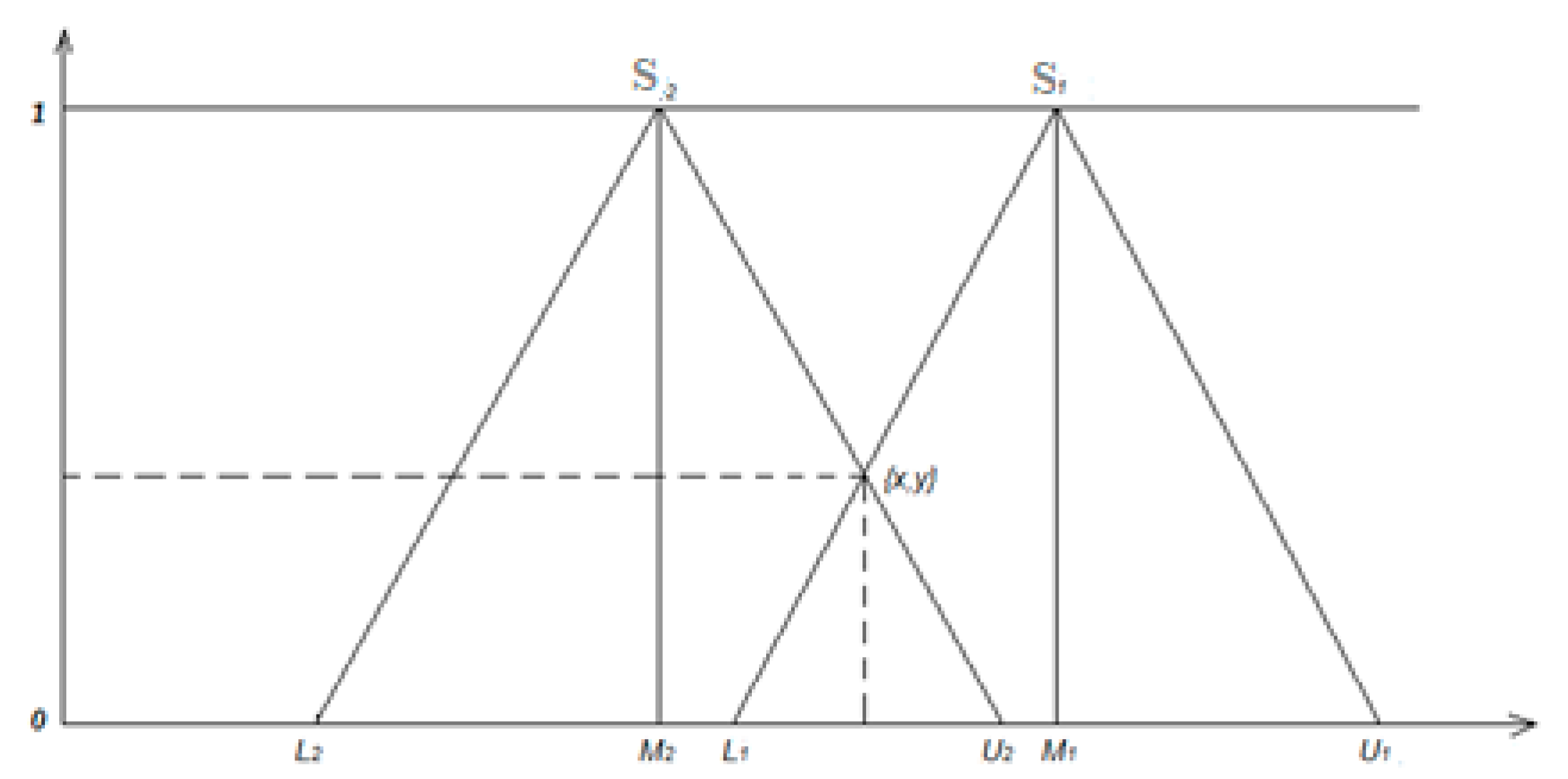
An important point in Chang’s proposed method for calculating the criteria weights is the comparison of ${\tilde{S}}_i,$ the extension of the fuzzy synthesis values (5). The essence of calculating the value of V (${\tilde{S}}_j\ge {\tilde{S}}_i$) is to find the ordinate of the intersection point of two triangular numbers (Figure 1). The triangles $S_1$ and $S_2$ do not intersect in the case when $L_1>U_2$. Then, with further calculation, using the formulas (4)–(8), the criterion weight is zero. That is, if a triangle does not intersect with at least one of the subsequent triangles, its weight is zero. This case is possible if the distance between the values $M_1$ and $M_2$ is large, and the triangles themselves are narrow (the distance from $L$ to $M$ and from $M$ to $U$ is 1), as in the case of the symmetric scale from Table 13. To give a better explanation of the case of zero weights when using narrow symmetric triangles, we will illustrate it with an example.

In solving real problems, when forming a fuzzy matrix from several AHP matrices, the $M$ values are most often averaged [49,51]. Chang’s work uses triangular numbers where the $M$ value does not exceed three [49].

In the following sections, symmetric and asymmetric triangular fuzzy numbers are used to form the AHP fuzzy matrix of pairwise comparisons. The implementation of the third algorithm will be illustrated using different matrices of pairwise comparisons, depending on the scale of the triangular fuzzy numbers used.

4.3.1. Using the Symmetric Scale for the Fuzzy Triangle

The fuzzy matrix (

Table 15. Pairwise comparison matrix using a symmetric triangular fuzzy numbers scale.

	1			2			3			4			5			6
1	1	1	1	1/6	1/5	1/4	1/3	1/2	1	1/5	1/4	1/3	1	2	3	3	4	5
2	4	5	6	1	1	1	3	4	5	1	2	3	6	7	8	8	9	9
3	1	2	3	1/5	1/4	1/3	1	1	1	1/3	1/2	1	3	4	5	4	5	6
4	3	4	5	1/3	1/2	1	1	2	3	1	1	1	4	5	6	6	7	8
5	1/3	1/2	1	1/8	1/7	1/6	1/5	1/4	1/3	1/6	1/5	1/4	1	1	1	1	2	3
6	1/5	1/4	1/3	1/9	1/9	1/8	1/6	1/5	1/4	1/8	1/7	1/6	1/3	1/2	1	1	1	1

) is formed in such a way that the most likely estimate of $M$ corresponds to the estimate of the AHP method. A 6 × 6 matrix with a good consistency index is used (Table 1). Fuzzy numbers replaces natural numbers, using the scales specified in Table 13 and Table 14, The remaining matrix estimates are calculated using the formula (4).

The matrix uses narrow symmetric triangular fuzzy numbers and a full scale of Saaty scores from 1 to 9. Systematically, we illustrate the calculation of weights using the Chang method.

Consider the summed values of $S_i=\sum _{i=1}^{\mathrm{m}}\sum _{j=1}^{\mathrm{m}}{\tilde{p}}_{ij}$ (

Table 16. Summed values of $S_i$.

	L	M	U
$S_1$	5.70	7.95	10.58
$S_2$	23.00	28.00	32.00
$S_3$	9.53	12.75	16.33
$S_4$	15.33	19.50	24.00
$S_5$	2.83	4.09	5.75
$S_6$	1.94	2.20	2.88

). The values of the number L of the second and fourth criteria ($S_2$,$S_4$) are very different from the other values of the L criteria. Note that the L value of the second criterion is greater than the U values of the first, third, fifth, and sixth criteria, and the L value of the fourth criterion is greater than the U values of the first, fifth and sixth criteria.

Further normalization, proposed by Chang, increases the values of U (dividing their values by the sum of the L numbers) and decreases the values of L (dividing the values by the sum of the U numbers). The values of M are normalized by dividing all elements by their sum, so the sum of the normalized values of M by all criteria is 1 (

Table 17. ${\tilde{S}}_i$ the extension of the fuzzy synthesis.

	$\widehat{\mathit{L}}$	$\widehat{\mathit{M}}$	$\widehat{\mathit{U}}$
${\tilde{S}}_1$	0.06	0.11	0.18
${\tilde{S}}_2$	0.25	0.38	0.55
${\tilde{S}}_3$	0.10	0.17	0.28
${\tilde{S}}_4$	0.17	0.26	0.41
${\tilde{S}}_5$	0.03	0.05	0.10
${\tilde{S}}_6$	0.02	0.03	0.05
Σ	0.64	1.00	1.57

).

For each i-th criterion, the value of ${\tilde{S}}_i$—the extension of the fuzzy synthesis—is calculated using the formula (5), and the specified answers are rounded.

$$\begin{array}{c}{\tilde{S}}_1=\left(5.7, 7.95, 10,58\right)\odot \left(\frac{1}{91.54},\frac{1}{74.5},\frac{1}{58,33}\right)=\left(0.06, 0.11, 0.18\right),\\ {\tilde{S}}_2=\left(23, 28, 32\right)\odot \left(\frac{1}{91.54},\frac{1}{74.5},\frac{1}{58,33}\right)=\left(0.25, 0.38, 0.55\right),\\ {\tilde{S}}_3=\left(9.53, 12.75, 16,33\right)\odot \left(\frac{1}{91.54},\frac{1}{74.5},\frac{1}{58,33}\right)=\left(0.1, 0.17, 0.28\right),\\ {\tilde{S}}_4=\left(15.33, 19.5, 24\right)\odot \left(\frac{1}{91.54},\frac{1}{74.5},\frac{1}{58,33}\right)=\left(0.17, 0.26, 0.41\right),\\ {\tilde{S}}_5=\left(2.83, 4.09, 5,75\right)\odot \left(\frac{1}{91.54},\frac{1}{74.5},\frac{1}{58,33}\right)=\left(0.03, 0.05, 0.1\right),\\ {\tilde{S}}_6=\left(1.94, 2.2, 2.88\right)\odot \left(\frac{1}{91.54},\frac{1}{74.5},\frac{1}{58,33}\right)=\left(0.02, 0.03, 0.05\right).\end{array}$$

The normalized summed values of ${\tilde{S}}_i$ are shown in Table 17. After normalization, the sum of the values of the triangular numbers is 0$<\Sigma \widehat{L}<$1,$\Sigma \widehat{M}=1$, and $\Sigma \widehat{U}>1$. Let us analyze how normalization changed the values of L and U, while expanding the values of the triangular numbers. Taking the example of the first criterion, the difference increased from $\frac{U_1}{L_1}=1.85$ to $\frac{{\widehat{U}}_1}{{\widehat{L}}_1}=3$. Unfortunately, normalization did not solve all the problems of the second and fourth criteria (${\widehat{L}}_2>{\widehat{U}}_1$, ${\widehat{L}}_2>{\widehat{U}}_5$, ${\widehat{L}}_2>{\widehat{U}}_6$, ${\widehat{L}}_4>{\widehat{U}}_5$, ${\widehat{L}}_4>{\widehat{U}}_6$). The inequalities show that the weights of the first, fifth, and sixth criteria will be zero. Further calculations will also show this.

To avoid this situation, it is recommended that, when using a narrow symmetric scale to fill in the matrix of pairwise comparisons, extreme/large values, such as (8, 9, 9), (7, 8, 9), and so on, are not used. Another possible way to avoid zero values is to use an asymmetric scale, which expands the triangle and the differences between the L and U values.

Then, using the extension of the fuzzy synthesis, all the criteria are compared in pairs using the formula (6):

$$\begin{array}{c}V\left({\tilde{S}}_1\ge {\tilde{S}}_2\right)=0, ({\widehat{L}}_2>{\widehat{U}}_1),\\ V\left({\tilde{S}}_1\ge {\tilde{S}}_3\right)=\frac{0.1 - 0.18 }{\left( 0.11 - 0.18 \right)-\left( 0.17 - 0.1\right)}=0.545,\\ V\left({\tilde{S}}_1\ge {\tilde{S}}_4\right)=\frac{0.17 - 0.18 }{\left( 0.11 - 0.18 \right)-\left( 0.26- 0.17\right)}=0.083,\\ V\left({\tilde{S}}_1\ge {\tilde{S}}_5\right)=1, ({\widehat{M}}_1>{\widehat{M}}_5),\\ V\left({\tilde{S}}_1\ge {\tilde{S}}_6\right)=1, \left({\widehat{M}}_1>{\widehat{M}}_6\right).\end{array}$$

$$V_1=\min \left(0, 0.545, 0.083, 1, 1\right)=0.$$

Then, a comparison is made in pairs of ${\tilde{S}}_2$ with all the other extensions of the fuzzy synthesis:

$$\begin{array}{c}V\left({\tilde{S}}_2\ge {\tilde{S}}_1\right)=1,\left({\widehat{M}}_2>{\widehat{M}}_1\right),\\ V\left({\tilde{S}}_2\ge {\tilde{S}}_3\right)=1, ({\widehat{M}}_2>{\widehat{M}}_3),\\ V\left({\tilde{S}}_2\ge {\tilde{S}}_4\right)=1, ({\widehat{M}}_2>{\widehat{M}}_4),\\ V\left({\tilde{S}}_2\ge {\tilde{S}}_5\right)=1, ({\widehat{M}}_2>{\widehat{M}}_5),\\ V\left({\tilde{S}}_2\ge {\tilde{S}}_6\right)=1, \left({\widehat{M}}_2>{\widehat{M}}_6\right).\end{array}$$

$$V_2=\min \left(1, 1, 1, 1, 1\right)=1.$$

Then, we carry out a pairwise comparison of ${\tilde{S}}_3$ with all the other values:

$$\begin{array}{c}V\left({\tilde{S}}_3\ge {\tilde{S}}_1\right)=1,\left({\widehat{M}}_3>{\widehat{M}}_1\right),\\ V\left({\tilde{S}}_3\ge {\tilde{S}}_2\right)=\frac{ 0.25- 0.28 }{\left( 0.17 - 0.28 \right)-\left( 0.38 - 0.25\right)}=0.123,\\ V\left({\tilde{S}}_3\ge {\tilde{S}}_4\right)=\frac{0.17- 0.28}{\left( 0.17- 0.28 \right)-\left( 0.26 - 0.17\right)}=0.554,\\ V\left({\tilde{S}}_3\ge {\tilde{S}}_5\right)=1, ({\widehat{M}}_3>{\widehat{M}}_5),\\ V\left({\tilde{S}}_3\ge {\tilde{S}}_6\right)=1, \left({\widehat{M}}_3>{\widehat{M}}_6\right).\end{array}$$

$$V_3=\min \left(1, 0.123, 0.554, 1, 1\right)=0.123.$$

Subsequent values $V_4, V_5, \mathrm{and} V_6$ are calculated in the same way. The following values are obtained: $V_4=\min \left(1, 0.584, 1, 1, 1\right)=0.584; V_5=\min \left(1, 0, 0.123, 0.584, 0\right)=0;$ $V_6=\min \left(0, 0, 0, 0, 0.42\right)=0;$ The vector of non-normalized criteria weights is $V$= (0, 1, 0.123, 0.584, 0, 0).

The vector of normalized criteria weights is obtained by applying formula (8): $w$= (0, 0.586, 0.072, 0.342, 0, 0).

In our further study of the stability of the AHP fuzzy method, we use the matrix from

Table 18. The third matrix of pairwise comparisons (6 × 6).

	cr1	cr2	cr3	cr4	cr5	cr6
cr1	1.00	0.33	0.50	2.00	1.00	2.00
cr2	3.00	1.00	1.00	2.00	2.00	3.00
cr3	2.00	1.00	1.00	2.00	1.00	2.00
cr4	0.50	0.50	0.50	1.00	0.50	1.00
cr5	1.00	0.50	1.00	2.00	1.00	2.00
cr6	0.50	0.33	0.50	1.00	0.50	1.00

, with a good consistency index (CR = 0.022).

Using the third algorithm, the stability of the method is also set by different numbers of iterations: 100, 10,000, and 100,000. The value of the largest relative errors ${\delta }^{\xi }$ of the values of the criteria weights is fixed. At least ten attempts are made to fix the interval of the largest relative errors, for non-zero values of the weights.

To analyze the stability with a symmetric scale of triangular numbers, we use the matrix presented in Table 18. When simulating an AHP matrix with 100 iterations, 60–70% of the subsequent matrices are consistent. The values of the weights of the initial fuzzy matrix criteria are 0.171, 0.288, 0.227, 0.071, 0.187, and 0.055. When calculating the criteria weights generated, and the matched pairwise comparison matrices, 70–80% of the matrices have zero weights, with the largest relative error being 1. The non-zero values of the weights and their largest relative errors are shown in

Table 19. The criteria weights of 5 matrices and the errors of the criteria weights when using a symmetric scale.

	$\mathit{\omega }$	1	2	3	4	5	δ
cr1	0.1715	0.2351	0.2535	0.214	0.1745	0.1204	0.9028
cr2	0.2882	0.2484	0.302	0.3236	0.2673	0.3304	0.439
cr3	0.227	0.1666	0.1753	0.0792	0.2576	0.277	0.651
cr4	0.0715	0.0552	0.0236	0.1181	0.1325	0.0258	0.8532
cr5	0.1868	0.1888	0.1939	0.2295	0.1568	0.222	0.8285
cr6	0.0551	0.106	0.0518	0.0356	0.0113	0.0245	0.9797

. The results show a high maximum relative error δ = 0.9797.

In general, the results for the relative errors of the third algorithm (Table 19), using a symmetric scale of triangular numbers, are greater than those for the first and second algorithms.

4.3.2. Using the Asymmetric Scale for the Fuzzy Triangle

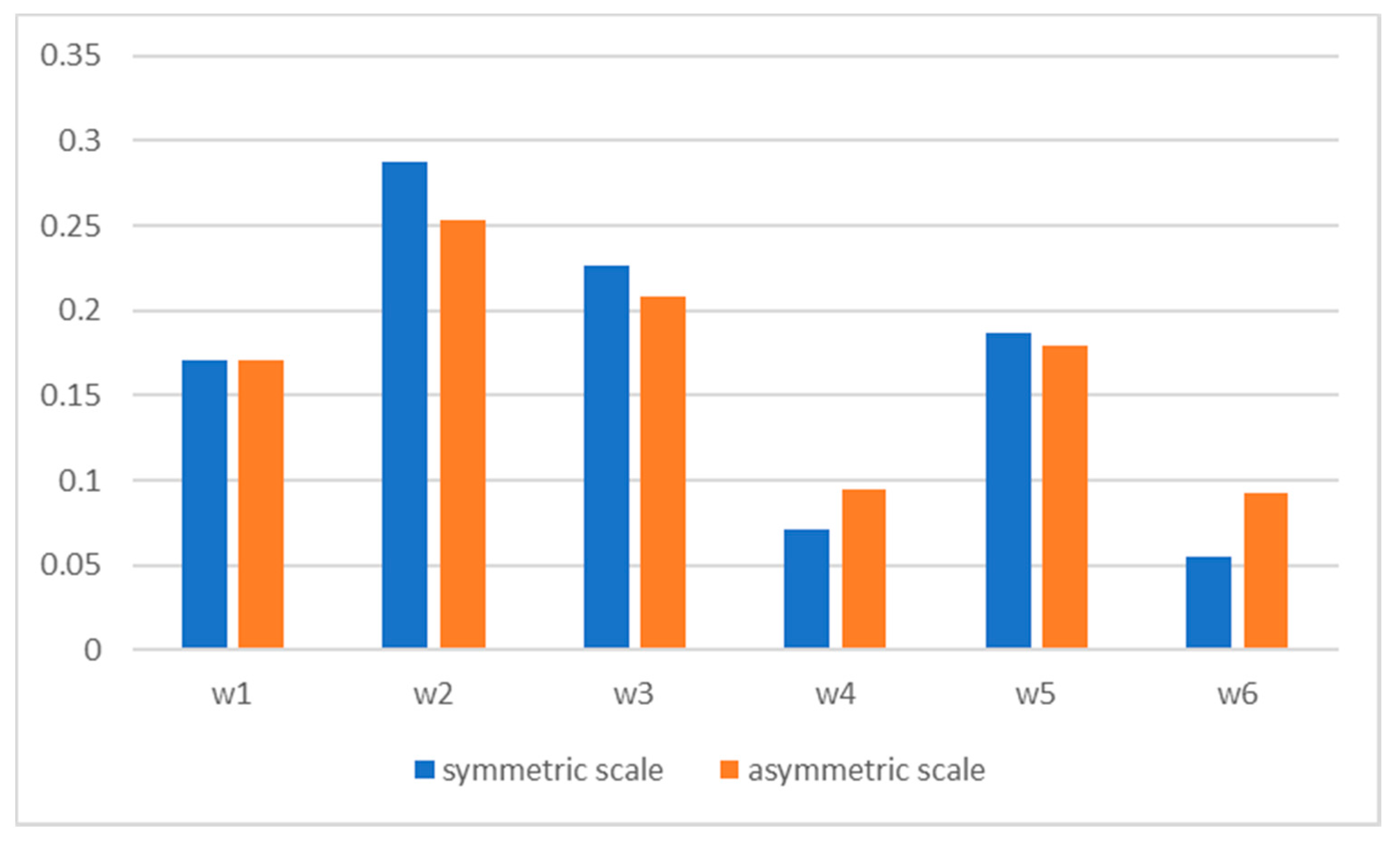
A fuzzy matrix using an asymmetric triangular scale is formed in the same way as a symmetric one, only using the scale from Table 14. The same 6 × 6 matrix with a good consistency index is used (Table 18). The values of the weights of the initial fuzzy matrix criteria are 0.171, 0.253, 0.208, 0.095, 0.179, and 0.093. In contrast to the symmetric scale, zero values of weights are extremely rare, 1–3%. The values of the criteria weights when using an asymmetric scale differ from the values obtained when using a symmetric one. However, the correlation coefficient of the weights obtained using symmetric and asymmetric scales is significant and is equal to 0.9987. The third matrix criteria weights were obtained using symmetric and asymmetric fuzzy scales from Table 13 and Table 14, shown in Figure 2.

The last check step was implemented to avoid zero weights using a symmetric scale using a third matrix with scores not exceeding 3. The result showed that the correlation of weights when using symmetric and asymmetric scales is high. Small changes to the symmetric scale do not significantly affect the scores, but they avoid zero weights.

Analyzing the results of 15 repetitions (100 iterations) (

Table 20. The largest relative errors of the criteria weights ${\delta }^{\xi }$, when checking the stability of the third algorithm, 100 iterations, 10 repetitions.

1	2	3	4	5	6	7	8	9	10
0.8933	0.7878	0.8397	0.9953	0.8933	0.6525	0.6052	0.6974	0.6496	0.7137
1.0924	1.1216	0.5863	1.0189	1.0446	0.6028	0.8377	0.6344	1.0367	0.5724
0.744	0.6998	0.7089	0.7983	0.7305	0.5985	0.6724	0.561	0.7166	0.6734
1.0571	0.8372	0.833	0.8002	0.8996	0.7833	0.6808	0.7526	0.8118	0.7294
0.891	0.6596	0.6372	0.768	0.891	0.6177	0.6831	0.5914	0.7144	0.6082
0.9636	0.7238	0.8619	0.9936	0.969	0.5921	0.8501	0.6585	0.7227	0.7013

), the values of the largest relative errors of the criteria weights of the second and fourth criteria are high, which means that the weights in some cases are more than doubled.

The results of the relative error intervals for different numbers of iterations are presented in

Table 21. The third algorithm, the largest ${\delta }^{\xi }$ relative errors of the criteria weights, 10 repetitions.

	100	10,000	100,000
cr1	0.6052–0.9953	1–1.0641	1.0338–1.0641
cr2	0.5724–1.1216	2.3281–2.9479	2.9479
cr3	0.561–0.7983	1–1.0442	1.0442
cr4	0.6808–1.0571	1.333–1.8541	1.8541
cr5	0.5914–0.891	1–1.332	1.332
cr6	0.5921–0.9936	1.0	1.0

. As the number of iterations increases, the largest relative errors also increase. The weights increase and decrease by almost a factor of two. The largest changes are for the weight value of the second criterion, by almost four times.

The use of an asymmetric scale of triangular numbers shows an improvement in the result compared to the results for the symmetric scale. There are practically no zero values of the weights, but even with a small fluctuation in the values of the matrix, the weights vary greatly. At the same time, the scale used in the AHP matrix varies from 1 to 4 or, respectively, fuzzy numbers from (1, 1, 1) to (3, 4, 5).

To further test the algorithm, the triangular values of fuzzy numbers are extended. We use the asymmetric scale from

Table 22. Asymmetrical scale of triangular fuzzy numbers.

Linguistic Characteristics of a Triangular Fuzzy Number	$\mathit{L}$	$\mathit{M}$	$\mathit{U}$
Equally important	1	1	3
Equally to moderately important	1	2	5
Moderately important	1	3	6
Weakly important	1	4	8
Important	2	5	8
Strongly important	2	6	9
Very important	5	7	9
Very strongly important	5	8	9
Absolutely important	7	9	9

, in order to avoid zero weights for the criteria of the first matrix (Table 1).

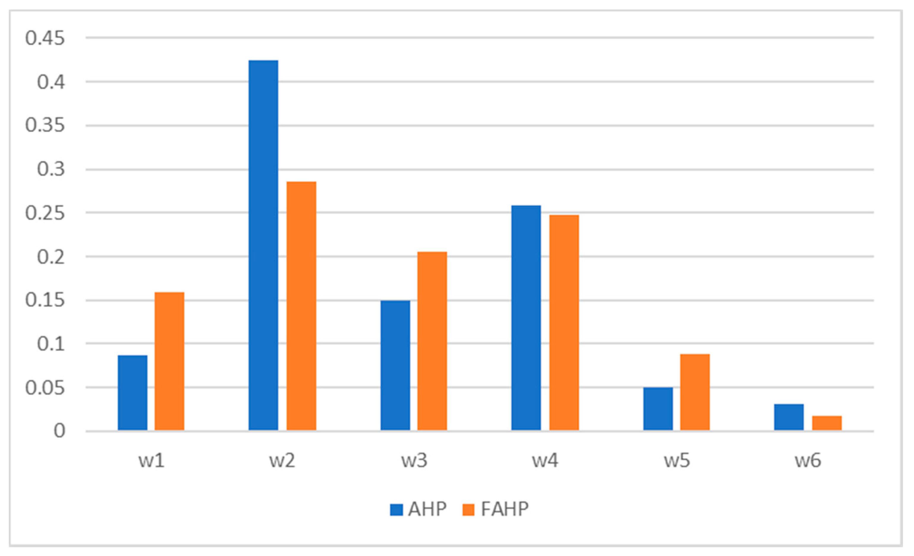
The initial values of M are used from the first matrix, which has a high consistency score (Table 1). The weights of the criteria of the fuzzy matrix that is formed when using triangular fuzzy numbers with the new scale in Table 22 are 0.159, 0.286, 0.205, 0.247, 0.088, and 0.017.

Figure 3 shows a greater degree of consistency of weight estimates by the AHP and FAHP methods using Chang’s algorithm. This result could not be predicted because Chang’s algorithm uses both different rating scales and the theory of comparing fuzzy numbers. The most significant difference in the weights of the first-matrix criteria obtained by the AHP and FAHP methods is observed in the first-third criterion.

An analysis of the values of ${\delta }^{\xi }$ for ten repetitions shows good results for the algorithm for criteria 1 to 5 (

Table 23. The third algorithm, ${\delta }^{\xi }$ the relative errors of the criteria weights, 100 iterations, 10 repetitions.

1	2	3	4	5	6	7	8	9	10
0.2421	0.273	0.3008	0.2018	0.2598	0.2718	0.2692	0.2421	0.2497	0.2522
0.1929	0.1782	0.1765	0.1852	0.1828	0.1695	0.181	0.1831	0.1824	0.1786
0.1594	0.1569	0.1559	0.1598	0.1525	0.153	0.1559	0.1506	0.153	0.1569
0.1561	0.1436	0.1468	0.1545	0.1395	0.1358	0.133	0.1553	0.1476	0.1521
0.5422	0.5217	0.5628	0.5514	0.5548	0.5434	0.5674	0.5776	0.5479	0.5947
4.3455	4.6545	4.0727	4.3697	4.0667	4.4788	4.0182	4.2788	3.9576	4.3212

). The large relative error values for the sixth criterion are explained by the fact that the weight in the original matrix is not large (${\omega }_{6 }=0.017$).

When checking the stability of the algorithm with a large number of iterations, the result remains the same, but the interval is narrowed to one value (

Table 24. The third algorithm, ${\delta }^{\xi }$ relative errors of the criteria weights, 10 repetitions.

	100	10,000	100,000
cr1	0.2018–0.3008	0.2957–0.3071	0.3071
cr2	0.1695–0.1929	0.1957–0.1992	0.1992
cr3	0.1506–0.1598	0.1618–0.1657	0.1657
cr4	0.133–0.1561	0.161–0.1675	0.1675
cr5	0.5217–0.5947	0.5959–0.6073	0.6073
cr6	3.9576–4.6545	4.5515–4.6606	4.6606

).

Despite the results for criterion 6 ($\delta =4.6606$), the weight of which varies from 0.017 to 0.08, the method using the new scale for forming triangular numbers shows a good result, comparable to the results of algorithms 1 and 2.

5. Discussion

Using the results of calculations of MCDM methods to choose the best alternative and to make the right decision makes practical sense if the models used are stable with respect to possible minor fluctuations in the initial data. Experts play a significant, and often crucial, role in the preparation of these MCDM methods. They form a set of criteria that characterize the process being evaluated. The criteria weights are usually calculated on the basis of their estimates, and often experts evaluate the values of the criteria themselves. Experts’ estimates are characterized by uncertainty. Therefore, when using MCDM methods, it is very important to investigate the influence of incomplete certainty about the data on the results of the calculations, and to assess the stability of the methods themselves.

The stability of MCDM models and the stability of the results depend both on the methods used and on the problem data themselves. Therefore, for each specific problem solved by MCDM, the use of methods for calculating the criteria weights and the specific methods for evaluating alternatives can be selected after checking these methods and the data for stability.

This paper should be considered as an integral part of the general task of studying the stability of MCDM models. For each specific MCDM method, it is necessary to investigate the stability of the weight estimates (this paper), as well as to evaluate the stability of the MCDM method itself. After that, the total error of the calculations can be estimated and the model with the smallest errors accepted.

A change often expresses the assessment of MCDM methods’ stability in the ranking of alternatives. In solving specific problems using many possible MCDM methods, the method’s result with the lowest degree of change of rang estimates is used.

Various methods can establish the weights of the criteria. Still, the AHP and FAHP methods’ peculiarity is in checking the consistency of expert assessments, which allows controlling the correctness of filling out the questionnaire.

The AHP method, as a mathematical method, shows a high degree of stability. This is to be expected: the method is mathematically justified, the elements of the matrix of the pairwise comparison of the criteria are ideally the ratio of the unknown criteria weights, and the weights themselves are normalized values of the eigenvector of the matrix.

Issues related to changes in the criteria weights that depend on ambiguous expert assessments have not received sufficient attention in the scientific literature. An expert, when filling out the same questionnaire again, usually fills it out a little differently. The errors in the calculated weights of the AHP method described in the second algorithm, which are related to the estimates of the experts themselves and the logic of their thinking, are significantly higher than the errors in the mathematical method itself. That, too, was to be expected. Reducing or increasing the comparative estimates of the experts by one significantly changes the values of the components of the eigenvector and the values of the criteria weights. The relative error of the weights increases. When comparing one criterion with all the others, the expert should also remember his previous assessments of the other criteria. With a large number of criteria, this task is not simple and often the comparison matrix is contradictory, not consistent. The expert is forced to fill in a new matrix, and his new estimates, of course, differ significantly from the original ones, as do the weights of the criteria. The relative error is quite large. It is possible to recommend that experts, before filling out an AHP matrix, rank the criteria according to their significance and, when filling out the matrix, constantly take into account the ranking results.

The greatest problems arise when evaluating the stability of the FAHP method weights. This is mainly due to the Chang algorithm used. Checking the AHP fuzzy method shows non-unambiguous results when using different scales of triangular numbers. In the analysis of the algorithm proposed by Chang for calculating weights, the possibility of zero weights for the criteria is emphasized. This is due to the possible excess of the value of L over U (L > U), which occurs because of the narrow scale of triangular numbers. Chang’s proposed algorithm includes normalization, which partially solves the problem of decreasing L and increasing U values, by expanding the triangular numbers and increasing the probability of an intersection of the ${\tilde{S}}_i$ values. This paper proposed an asymmetric scale of triangular numbers, which excluded the appearance of zero weights. At the same time, the calculated fuzzy weights correlated well with the weights of the AHP method. In subsequent work, the authors plan to study in more detail the influence on the final result of the scale used for the triangular numbers and suggest other ways of normalization, to avoid zero values for the criteria weights. Chang’s algorithm is also sensitive to large estimates from the Saaty scale (close to 9), in which case the criteria weights can take zero values.

The criteria weights calculated using the AHP and FAHP methods are naturally different, but as the average M values of the FAHP matrix coincide with the values of the AHP matrix, the weights of the two methods should correlate with each other. However, when some of the criteria weights are zero, there is no need to talk about compliance. The situation is “corrected” by the use of the asymmetric scale proposed in this article.

The order of significance of the criteria weights of the first matrix calculated by the AHP and FAHP methods coincided: (cr2 $\succ$ cr $\succ$ cr3 $\succ$ cr1 $\succ$ cr5 $\succ$ cr6). The correlation coefficient of the AHP weights (0.0873, 0.4246, 0.149, 0.2585, 0.0496, 0.0311) and the FAHP scales ( 0.159, 0.286, 0.205, 0.247, 0.088, 0.017) is large enough and equal to 0.8894.

A review of the scientific literature confirms the relevance of the problems studied in this paper. Despite the presence of papers that use a stability check for the AHP method, the results of the algorithms could not be compared because of different interpretations of the results. Noted that despite the widespread use of the FAHP method, little attention has been paid to checking its stability, so the results of this paper are of scientific interest.

The theory of interval numbers is a universal approach for solving many applied problems. The FAHP method is useful for solving problems using linguistic scales that cannot be written down in a single number. In this case, the sensitivity test of the FAHP method to select the scale of triangular numbers is recommended. Otherwise, the AHP method is recommended.

6. Conclusions

The stability of multicriteria MCDM methods is associated with the incomplete certainty of the data used for calculations.

This uncertainty is particularly evident when calculating the subjective weights of criteria based on expert assessments. Unstable estimates (ranking) in MCDM methods reduce the quality of the estimates and the reliability of the decision. The instability of the MCDM methods can result in an incorrect ranking of the evaluated alternatives, not the proper choice of the best option, inaccurate estimates of the criteria’ significance, and the criteria weights’ values in a particular situation and environment. Therefore, the problem investigated in this publication is relevant. The calculations show that the AHP method, as a mathematical method, is stable with respect to minor fluctuations in the elements of the comparison matrix. The transition from the Saaty scale integers 1-3-5-7-9 to close real numbers slightly changes the values of the weights. The relative error of the weight estimates that were insignificant varied between δ = 0.0531 (at 5% deviation) and δ = 0.116 (at 10% deviation).

The maximum relative error of the AHP method, related to the assessments of the experts themselves, the logic of their thinking, and psychology, is significantly greater than the error of AHP as a mathematical method. At the same time, changing the elements of the comparison matrix by units significantly affects the values of the eigenvector components of the matrix. The relative error of the estimates of the weights much higher and varied in the range δ = 0.5121 to δ = 0.7739.

The stability of the weights of the FAHP method is related not only to the factors listed above for the AHP method, but also to the use of Chang’s algorithm for estimating weights. The calculations show that the algorithm itself is not universal, is not applicable for all matrices, and depends on the scale used for the estimates of the triangular numbers. If the evaluation scale is incorrectly selected, the weights may be zero for some matrices. The relative error of the FAHP method is significantly higher than that for the AHP method and varied from δ = 0.2421 to δ = 0.9797. It was anomalous (δ = 4.6606) in the case of a very small weight for a criterion.

The proposed asymmetric FAHP scale significantly improved the results: it eliminated the appearance of zero weights for criteria, reduced the values of the maximum relative errors, and showed a high degree of correlation with the weights obtained by the AHP method.

Regarding the novelty and relevance of this paper, we can point to the study of the stability of the AHP method, which depends on the instability of the estimates of the experts themselves, and the analysis of the stability of the FAHP method, which was clearly insufficiently studied earlier. This paper can be used to analyze the stability of specific MCDM methods by ranking the alternatives.