Article

Controlling Wolbachia Transmission and Invasion Dynamics among Aedes Aegypti Population via Impulsive Control Strategy

by
Joseph Dianavinnarasi
1,
Ramachandran Raja
2,
Jehad Alzabut
3,*,
Michał Niezabitowski
4 and
Ovidiu Bagdasar
5
1
Department of Mathematics, Alagappa University, Karaikudi 630 004, India
2
Ramanujan Centre for Higher Mathematics, Alagappa University, Karaikudi 630 004, India
3
Department of Mathematics and General Sciences, Prince Sultan University, Riyadh 12435, Saudi Arabia
4
Department of Automatic Control and Robotics, Faculty of Automatic Control, Electronics and Computer Science, Silesian University of Technology, Akademicka 16, 44-100 Gliwice, Poland
5
Department of Electronics, Computing and Mathematics, University of Derby, Derby DE22 1GB, UK
*
Author to whom correspondence should be addressed.
Symmetry 2021, 13(3), 434; https://doi.org/10.3390/sym13030434
Submission received: 15 February 2021 / Revised: 2 March 2021 / Accepted: 3 March 2021 / Published: 8 March 2021
(This article belongs to the Special Issue Multibody Systems with Flexible Elements)

Abstract

:
This work is devoted to analyzing an impulsive control synthesis to maintain the self-sustainability of Wolbachia among Aedes Aegypti mosquitoes. The present paper provides a fractional order Wolbachia invasive model. Through fixed point theory, this work derives the existence and uniqueness results for the proposed model. Also, we performed a global Mittag-Leffler stability analysis via Linear Matrix Inequality theory and Lyapunov theory. As a result of this controller synthesis, the sustainability of Wolbachia is preserved and non-Wolbachia mosquitoes are eradicated. Finally, a numerical simulation is established for the published data to analyze the nature of the proposed Wolbachia invasive model.

1. Introduction

In the 19th century, fractional calculus (FC) theory has been built by some famous mathematicians like Grunwald, Letnikov, Riemann, Liouville, Euler and Caputo [1,2,3]. Fractional order derivatives are the generalization of integer order derivatives. FC is unavoidable due to its extensive applications in the study of real-world problems. The main advantage of FC is that it can provide a path to understand the description of memory and inheritance of various processes [4,5]. The book [6] plays an important role in the area of applied fractional calculus. In recent years, researchers in the field of physics, chemistry, Neural Networks, economic and mathematical modeling, biological problems and engineering have been very much attracted to fractional calculus [7], because FC interprets the whole function geometrically and globalizes its entire function.
Mosquito-borne diseases are primarily spread by female mosquitoes while taking a blood meal from living organisms such as humans, animals and birds. A parasite, virus, or bacteria-infected female mosquito can transmit those foreign agents to humans [8]. For instance, the Dengue virus, Zika virus, Yellow fever virus and Chikungunya are transmitted from infected human to uninfected human via primary vector Aedes Aegypti mosquitoes. Currently, the secondary vector for the above-mentioned diseases is Aedes Albopictus [9,10,11]. In recent years, the death rate due to mosquito-borne diseases has increased dramatically [8]. Gubler et al. [12,13] and Ong et al. [14] explained that dengue and dengue hemorrhagic fever are a more common issue for public health. According to the World Health Organization (WHO) [15], per annum, mosquito-borne diseases cause more than 40,000 deaths and 96 million asymptomatic cases in 129 countries.
Currently, there are several methods to control Aedes Aegypti mosquitoes such as insecticide spraying, sterile insect technique, incompatible insect technique, combined sterile insect technique, and genetic modifications. In [16,17], the authors proposed that the Sterile insect technique is likely to be used in mosquito-borne disease control. The authors of [18], analyzed that the particular transgenic strain can simulate the female-specific flightless phenotype to increase the sterilization in male mosquitoes. In [19,20], the authors discussed that the safe and effective replacement of vector population by genetically modified mosquitoes will play a significant role in mosquito-borne disease control. Furthermore, some other types of mosquito control strategies, such as making changes in feeding behaviors, intervention strategies, using bed nets and mosquito repellents, are also tested [21,22].
A novel Aedes Aegypti suppression technique using the life-shortening bacterium Wolbachia plays an important role [23,24,25]. It is an endosymbiotic bacterium that is reported in nearly 60 percent of insect species by Wolbach (1924) [26]. The World Mosquito Program (WMP) [27] from Australia currently release Wolbachia infected mosquitoes over 10 countries, such as countries in Latin America, India, Sri Lanka, Vietnam, Indonesia and cities in Oceania. In that research, they found that Wolbachia is a self-sustaining bacterium and in the presence of Wolbachia infected mosquitoes there is zero possibility of having Dengue. The Wolbachia releasing strategy is more powerful than that of the above-mentioned control strategies in the sense that it is self-sustaining, affordable, only needs a small amount of release, the area covered is larger than the released area, and the most important thing is it is not harmful to human health. The authors of [28,29,30,31] discussed that Wolbachia can restrict the virus particles of various diseases. We know that the virus is transmitted from infected humans to uninfected humans via female mosquitoes. Meanwhile, if a virus-infected mosquito carries Wolbachia strain, then the virus cannot be transmitted to an uninfected human. Because this Wolbachia strain blocks the virus particles inside the salivary gland of mosquitoes (Ref. Figure 1).
The Wolbachia infection is introduced into wild mosquitoes population through two major processes such as microinjection and Introgression [32].
  • Micro injection: In this process, Wolbachia strains are microinjected into aquatic stages such as eggs, larvae and pupae.
  • Introgression: In this process, the Wolbachia strains are carried out to next generation through mating. If Wolbachia infected female mated with Wolbachia infected or uninfected male, then the produced offsprings have the Wolbachia strain (Called CI rescue). Suppose the Wolbachia uninfected female mated with a Wolbachia infected male then there is no viable progeny. Finally, if a non-Wolbachia female mated with a non-Wolbachia male then there is no Wolbachia infection in the offspring.
To understand the introgression process, one can refer to Figure 2.
Furthermore, some existing mathematical models consider Wolbachia as a control agent for mosquito-borne diseases. In [33], the author proposed a deterministic model to control mosquito-borne diseases up to 90% via Wolbachia spread, also the author considered both human and mosquito populations to create a mathematical model. In [30,34], the authors proposed a mathematical model depicting the life stages of mosquitoes with Wolbachia and proved that Wolbachia has an excellent quality to control dengue virus spread. In [35], the authors analyzed the integer ordered mathematical model consisting of only four stages (aquatic stage with and without Wolbachia and adult female mosquitoes with and without Wolbachia), which considered the imperfect maternal transmission and Wolbachia invasion. In [36], the two sex mathematical model is discussed to analyze the persistence of Wolbachia. In [37], the age and bite structured mathematical model is proposed and performed the mathematical analysis. In [38], the authors discussed the linear feedback control strategy of a mathematical model containing only three stages such as aquatic, female Wolbachia infected and uninfected mosquitoes. In this, the author analyzed the Wolbachia infected mosquitoes release into the seasonal environment. In [39], the authors presented a mathematical model to depict the mechanism of the virus inside both humans and mosquitoes. In this work, the author utilized two various types of controls like vaccination for humans and Wolbachia infected mosquitoes’ release for mosquitoes. The pontriyagin maximum principle was utilized to analyze the optimal control of the proposed mathematical model. In [40], the authors discussed the Wolbachia infection among Aedes Aegypti mosquitoes via delay differential equations. In that work, the author proposed the delay dependent stability criteria of the proposed model by utilizing the results from spectrum analysis. In [41], the authors proposed an age structured fractional order mathematical model to control the Aedes Aegypti mosquitoes via Wolbachia bacterium using the Linear Matrix Inequality (LMI) approach.
As per the practical results of [27], Wolbachia should be released into every stage to get the optimal control in a short period. Also, by utilizing fractional calculus we can get the memory property and inheritance of this process. In nature, Wolbachia infected mosquitoes may lose the Wolbachia infection. Because of this, invasion in Wolbachia is unavoidable. Motivation by the above discussions, our contributions are listed below:
  • A novel mathematical model, which considers the total of ten stages in Aedes Aegypti mosquitoes (combining both Wolbachia infected and Wolbachia uninfected) is proposed and the possible optimal stages to release the Wolbachia are discussed, and the most important concept of Wolbachia invasion and Wolbachia gain are adopted.
  • The Wolbachia free equilibrium, Wolbachia present Equilibrium, Zero mosquitoes, and both Wolbachia and Non-Wolbachia mosquitoes co-existence equilibrium are derived. And utilizing fixed point theory results, the Existence and Uniqueness results of the Wolbachia invasive model are proposed. To attain optimal control, we utilized an impulsive control strategy.
  • We perform global Mittag-Leffler stability analysis of the proposed model via Linear Matrix Inequality (LMI) theory and Lyapunov theory.
  • In the end, by utilizing the data from the published literature, we have presented the numerical simulation of the proposed model using MATLAB software.
The rest of the paper is arranged as follows—in Section 2, we provide some basic Definitions, Lemmas and Theorems. In Section 3, the fractional order complete mathematical model describes the interaction between Wolbachia infected and Non-Wolbachia mosquitoes is presented. In Section 4, the possible equilibrium points are presented. In Section 5, the Wolbachia invasive and gain model with impulsive control is presented. In Section 6, the existence and uniqueness results are analyzed and the global Mittag-Leffler stability results are derived in Section 7. In Section 8, the numerical simulation results are presented. In Section 9, the work is concluded.
Notations. N denotes the space of all natural numbers, R denotes the space of all real numbers, C denotes the space of all complex numbers, R n denotes the space of n-dimensional Euclidean space, Z + denotes the space of all positive integers. Moreover, R e ( · ) denotes the real part of a complex number and [ . ] denotes the integer part of a number. * denotes the corresponding symmetric terms in a symmetric matrix. Also, k c D t α ( · ) and k c I t α ( · ) denotes the derivative and anti derivative of order α with respect to t respectively, c denotes that its in Caputo sense, k denotes the initial condition and Γ ( · ) denotes the Gamma function.

2. Preliminaries

In this section, we provide some basic Definitions, Lemmas and Theorems, which are used to attain our results.
Definition 1.
Ref. [4] The most important basic function in fractional calculus is the gamma function. It is defined as follows:
Γ ( z ) = 0 e s s z 1 d s ,
with R e ( z ) > 0 .
Definition 2.
Ref. [1] The Caputo fractional derivative of a continuous function f ( t ) over [ k , T ] of order α C (with R e ( α ) > 0 , α N ) is
k c D t α f ( t ) = 1 Γ ( n α ) k t ( t η ) n α 1 d n d η n f ( η ) d η ,
where, n = [ R e ( α ) ] + 1 .
If 0 < R e ( α ) < 1 , then the expression (1), can be rewritten as
k c D t α f ( t ) = 1 Γ ( 1 α ) k t f ( η ) d η ( t η ) α .
Since, n = 1 for all 0 < R e ( α ) < 1 .
Definition 3.
Ref. [42] The Caputo sense fractional integral of a continuous function f on L 1 ( [ 0 , T ] , R ) over α ( 0 , 1 ] with respect to t is defined as
0 c I t α f ( t ) = 1 Γ ( α ) 0 t ( t η ) α 1 f ( η ) d η .
The two parameter Mittag-Leffler function is defined as follows: [4]
E a , b ( z ) = l = 0 z l Γ ( a l + b ) ,
where, z C , a > 0 , and b > 0 . If b = 1 the E a ( z ) = l = 0 z l Γ ( a l + 1 ) . If both a = 1 and b = 1 , the E 1 , 1 ( z ) = e z .
Lemma 1
(Schur Complement [43]). Let us denote three n × n matrices as Ψ 1 , Ψ 2 , Ψ 3 , where Ψ 1 = Ψ 1 and Ψ 2 = Ψ 2 > 0 . Then Ψ 1 + Ψ 3 Ψ 2 1 Ψ 3 < 0 if and only if Ψ 1 Ψ 3 Ψ 3 Ψ 2 < 0 (or) Ψ 2 Ψ 3 Ψ 3 Ψ 1 < 0 .
Lemma 2.
Ref. [44] For any scalar ϵ > 0 , A , N R n and matrix P 1 , then
A P 1 N 1 2 ϵ A P 1 P 1 A + ϵ 2 N N .
Let us consider the fractional order dynamical system with impulse of type,
k c D t α x ( t ) = A 1 x ( t ) + A 2 f ( x ( t ) ) , t t θ , θ = 1 , 2 , , m , Δ x ( t θ ) = x ( t θ + ) x ( t θ ) = δ θ ( x ( t θ ) ) , t = t θ , θ = 1 , 2 , , m ,
with initial condition x ( t 0 ) = x 0 Z + , where the n states is defined by x ( t ) = [ x 1 ( t ) , x 2 ( t ) , x 3 ( t ) , , x n ( t ) ] R n and f ( x ( t ) ) = [ f ( x 1 ( t ) ) , f ( x 2 ( t ) ) , f ( x 3 ( t ) ) , , f ( x n ( t ) ) ] be a function, A 1 and A 2 are constant coefficient matrices with the impulsive operator δ θ : R n R n .
Definition 4.
Ref. [44] The system (4), is said to be globally Mittag-Leffler stable at its equilibrium points, if the following hold:
| | x ( t ) x * | | h ( x 0 x * ) E α ( κ t a ) b ,
where x * is an equilibrium point, 0 < α < 1 , κ 0 and a , b > 0 . Moreover, h ( 0 ) = 0 , h ( x ) 0 and h ( x ) is locally Lipschitz with Lipchitz constant h 0 .
Lemma 3.
Ref. [45] Let us consider the fractional order system with impulsive control of type (4). Suppose f ( 0 ) = 0 , t > 0 and δ θ ( 0 ) = 0 , θ = 1 , 2 , 3 , , m . If there exists a positive definite function V such that the following hold:
(1) 
There exists positive constants α 1 and α 2
α 1 | | x ( t ) | | V ( t ) α 2 | | x ( t ) | | , x ( t ) R n .
(2) 
0 c D t α V ( t ) ϵ 1 V ( t ) , t t θ , θ = 1 , 2 , 3 , , m for any scalar ϵ 1 .
(3) 
V ( t θ + ) V ( t θ ) , t = t θ , θ = 1 , 2 , 3 , , m .
then the equilibrium point of the system (4) is globally Mittag-Leffler stable.
Definition 5.
Ref. [46] A map ν : H H , H compact Banach space, is said to be a contraction mapping if there exists h ( 0 , 1 ) such that
| | ν ( m 1 ) ν ( m 2 ) | | h | | m 1 m 2 | |
for every m 1 , m 2 H .
Theorem 1
(Contraction Mapping Theorem). Ref. [46] Suppose H is a complete metric space and ν : H H is a contraction mapping. Then, ν has a unique fixed point.

3. Model Formulation

In this section, a novel mathematical model is proposed to expose the transmission dynamics of the gram negative bacteria Wolbachia among Aedes Aegypti mosquitoes. While constructing the model we have considered the total of 10 stages such as non-Wolbachia eggs ( W e ) , non-Wolbachia larvae ( W l ) , non-Wolbachia pupae ( W p ) , non-Wolbachia adult female ( W f ) , non-Wolbachia adult male ( W a ) , Wolbachia infected eggs ( I e ) , Wolbachia infected larvae ( I l ) , Wolbachia infected pupae ( I p ) , Wolbachia infected adult female ( I f ) , Wolbachia infected adult male ( I a ) . The total population at time t is denoted as T = W e ( t ) + W l ( t ) + W p ( t ) + W f ( t ) + W a ( t ) + I e ( t ) + I l ( t ) + I p ( t ) + I f ( t ) + I a ( t ) . The eggs with zero Wolbachia infection are produced at the rate Λ w e by the mating process between non-Wolbachia female ( W f ) and non-Wolbachia male ( W a ) . There is no other possibilities of having a non-Wolbachia eggs. Therefore, the reproduction rate of non-Wolbachia mosquitoes can be calculated by the term Λ w e W f W a T . Along with this, the terms λ w e (natural mortality rate of non-Wolbachia eggs) and γ w e (maturation rate of non-Wolbachia eggs) denotes the limitations in the growth of wild mosquito eggs. At the same time, after release of Wolbachia infected mosquitoes (in both aquatic and ariel stage) in a common environment, the production of Wolbachia infected mosquito eggs I e ( t ) , depends on mating between Wolbachia infected female I f ( t ) and non-Wolbachia male W a ( t ) and from mating between Wolbachia infected female I f ( t ) and Wolbachia infected male I a ( t ) . Through this, the birth rate of Wolbachia infected mosquito eggs population I e ( t ) with the reproduction rate Λ i e is
Λ i e ( I f W a + I f I a ) T = Λ i e I f ( W a + I a ) T .
Similarly, the increase in the growth of Wolbachia infected eggs is limited by the natural mortality rate λ i e and the maturation rate γ i e (That is, the rate in which the corresponding compartment moved into the next stage).
Furthermore, the quantity ( 1 α ) γ i e I e is added to the wild mosquito larvae population. Because the term α and ( 1 α ) denotes the probability of getting larvae with and without Wolbachia respectively. Similarly, β and ( 1 β ) denotes the probability of getting pupae with and without Wolbachia respectively, ϵ and ( 1 ϵ ) denotes the probability rate of having Wolbachia infection in adult mosquitoes by introgression. That is, ϵ be the probability of getting Wolbachia infected adults (with ρ i w = probability of getting male and ( 1 ρ i w ) = probability of getting female). Because of these reasons, the terms ( 1 α ) γ i e I e , ( 1 β ) γ i l I l , ( 1 ϵ ) γ i p ρ i w I p and ( 1 ϵ ) γ i p ( 1 ρ i w ) I p are added to the corresponding stages and similarly, the terms α γ i e I e , β γ i l I l and ϵ γ i p I i p are removed from the corresponding stages. The parameter description of the system of Equation (5) is presented in Table 1.
From the above facts, the novel mathematical model that describes the transmission dynamics of Wolbachia among Aedes Aegypti mosquitoes is proposed as follows:
0 c D t α W e = Λ w e W f W a T λ w e W e γ w e W e 0 c D t α W l = γ w e W e λ w l W l γ w l W l + ( 1 α ) γ i e I e 0 c D t α W p = γ w l W l λ w p W p γ w p W p + ( 1 β ) γ i l I l 0 c D t α W f = ρ γ w p W p λ w f W f + ( 1 ϵ ) γ i p ρ i w I p 0 c D t α W a = ( 1 ρ ) γ w p W p λ w a W a + ( 1 ϵ ) γ i p ( 1 ρ i w ) I p 0 c D t α I e = Λ i e I f ( W a + I a ) T λ i e I e α γ i e I e 0 c D t α I l = α γ i e I e λ i l I l β γ i l I l 0 c D t α I p = β γ i l I l λ i p I p ϵ γ i p I p 0 c D t α I f = ρ i ϵ γ i p I p λ i f I f 0 c D t α I a = ( 1 ρ i ) ϵ γ i p I p λ i a I a .
The dynamics of the population can be easily understand by the schematic diagram Figure 3 and the parameters are described in Table 1.

4. Equilibrium Points

In this section, we can find the four cases of possible equilibrium points such as wild mosquitoes only, Wolbachia mosquitoes only, co-existence of both population and zero mosquitoes.

4.1. Zero Mosquitoes

Suppose there is no mosquitoes, then the equilibrium point can be written as P 1 = ( 0 , 0 , 0 , 0 , 0 , 0 , 0 , 0 , 0 , 0 ) . This is trivial but does not exists in nature.

4.2. Wolbachia Infected Mosquitoes Free Equilibrium

Suppose, there is no Wolbachia infected mosquitoes population then the possible equilibrium can be written as
P 2 = ( W e 1 * , W l 1 * , W p 1 * , W f 1 * , W a 1 * , 0 , 0 , 0 , 0 , 0 ) ,
where,
W e 1 * = T λ w f λ w a ( λ w e + γ w e ) ( λ w l + γ w l ) 2 ( λ w p + γ w p ) 2 ρ ( 1 ρ ) Λ w e γ w p 2 γ w e 2 γ w l 2 W l 1 * = γ w e λ w l + γ w l W e 1 * W p 1 * = γ w l γ w e ( λ w l + γ w l ) ( λ w p + γ w p ) W e 1 * W f 1 * = ρ γ w p γ w e γ w l λ w f ( λ w f + γ w f ) ( λ w p + γ w p ) W e 1 * W a 1 * = ( 1 ρ ) γ w p γ w e λ w e ( λ w l + γ w l ) ( λ w p + γ w p ) W e 1 *

4.3. Wild Mosquitoes Free Equilibrium

After the successful replacement of Wolbachia uninfected mosquitoes by Wolbachia infected mosquitoes the equilibrium point can be represented by
P 3 = ( 0 , 0 , 0 , 0 , 0 , I e 2 * , I l 2 * , I p 2 * , I f 2 * , I a 2 * ) ,
where,
I e 2 * = ( λ i l + β γ i l ) ( λ i p + ϵ γ i p ) α β γ i e γ i l I p 2 * I l 2 * = ( λ i p + ϵ γ i p ) β γ i l I p 2 * I p 2 * = T λ i f λ i a ( λ i e + α γ i e ) ( λ i l + β γ i l ) ( λ i p + ϵ γ i p ) Λ i e α β ρ i ( 1 ρ i ) ϵ 2 γ i p 2 γ i e γ i l I f 2 * = ρ i ϵ γ i p λ i f I p 2 * I a 2 * = ( 1 ρ i ) ϵ γ i p λ i a I p 2 * .

4.4. Both Wolbachia Infected Mosquitoes and Non-Wolbachia Mosquitoes Co-Existence Equilibrium

If both Wolbachia infected and Wolbachia uninfected mosquitoes present in common environment, then the equilibrium point is
S n = W e n * , W l n * , W p n * , W f n * , W a n * , I e n * , I l n * , I p n * , I f n * , I a n * , n = 3 , 4 .
W e n * = λ w l + γ w l γ w e λ w p + γ w p γ w l T B 1 B 2 B 3 λ i f λ w a Λ i e ( 1 ρ ) ρ i γ w p I a n * γ w e B 4 ( λ w l + γ w l ) λ w p + γ w p γ w l + ( λ w l + γ w l ) ( 1 β ) γ i l γ w l λ i a B 1 β γ i l ( 1 ρ i ) + ( 1 α ) γ i e λ i a B 1 B 2 α γ i e ( 1 ρ i )
W l n * = λ w p + γ w p γ w l T B 1 B 2 B 3 λ i f λ w a Λ i e ( 1 ρ ) ρ i γ w p B 4 I a n * ( 1 β ) γ i l γ w l λ i a B 1 β γ i l ( 1 ρ i )
W p n * = T B 1 B 2 B 3 λ i f λ w a Λ i e ( 1 ρ ) ρ i γ w p B 4 I a n *
W f n * = ρ γ w p λ w f T B 1 B 2 B 3 λ i f λ w a Λ i e ( 1 ρ ) ρ i γ w p B 4 I a n * + ( 1 ϵ ) ρ i w λ i a ϵ λ w f ( 1 ρ i ) I a n *
W a n * = T B 1 B 2 B 3 λ i f ρ i Λ i e I a n *
I e n * = B 1 B 2 λ i a I a n * α γ i e ( 1 ρ i )
I p n * = λ i a ( 1 ρ i ) ϵ γ i p I a n *
I f n * = ρ i λ i a I a n * ( 1 ρ i ) λ i f
with I a 3 * > I a 4 * , both roots can be found from the quadratic equation
a 1 I a * 2 + a 2 I a * + a 3 = 0 ,
where,
a 1 = Λ w e ρ B 4 γ w p T λ w f ; a 2 = λ w e + γ w e T λ w f λ w e λ i f ρ B 1 B 2 B 3 ρ i Λ i e λ w f λ w a ( 1 ρ ) + B 4 γ w p ( λ w l + γ w l ) ( λ w p + γ w p ) B 4 γ w l + ( λ w l + γ w l ) ( 1 β ) λ i a B 1 γ w l β ( 1 ρ i ) + ( 1 α ) λ i a B 1 B 2 α ( 1 ρ i ) ; a 3 = Λ w e ρ T B 1 2 B 2 2 B 3 2 λ w a Λ i e 2 ( 1 ρ ) ρ i 2 λ w f .
Here,
B 1 = 1 + λ i p ϵ γ i p ; B 2 = 1 + λ i l β γ i l ; B 3 = 1 + λ i e α γ i e ; B 4 = 1 + ( 1 ϵ ) ( 1 ρ i w ) λ i a ( 1 ρ ) ( 1 ρ i ) ϵ γ w p .
For more details about the calculations of Section 4, kindly refer the Appendix A section.

5. Wolbachia Invasion Model

We considered the possibility of Wolbachia loss in adult mosquitoes and possibility of Wolbachia gain in aquatic stage mosquitoes. Then Equation (5), can be rewritten as
0 c D t α W e ( t ) = Λ w e W f W a T λ w e W e γ w e W e η 1 I e 0 c D t α W l ( t ) = γ w e W e λ w l W l γ w l W l + ( 1 α ) γ i e I e η 2 I l 0 c D t α W p ( t ) = γ w l W l λ w p W p γ w p W p + ( 1 β ) γ i l I l η 3 I p 0 c D t α W f ( t ) = ρ γ w p W p λ w f W f + ( 1 ϵ ) γ i p ρ i w I p + η 4 W f 0 c D t α W a ( t ) = ( 1 ρ ) γ w p W p λ w a W a + ( 1 ϵ ) γ i p ( 1 ρ i w ) I p + η 5 W a 0 c D t α I e ( t ) = Λ i e I f ( W a + I a ) T λ i e I e α γ i e I e + η 1 I e 0 c D t α I l ( t ) = α γ i e I e λ i l I l β γ i l I l + η 2 I l 0 c D t α I p ( t ) = β γ i l I l λ i p I p ϵ γ i p I p + η 3 I p 0 c D t α I f ( t ) = ρ i ϵ γ i p I p λ i f I f η 4 W f 0 c D t α I a ( t ) = ( 1 ρ i ) ϵ γ i p I p λ i a I a η 5 W a ,
where η 1 , η 2 and η 3 all are the rates at which the non-Wolbachia aquatic population gain Wolbachia infected mosquitoes infection and η 4 & η 5 are the rates at which the Wolbachia infected mosquitoes losses their Wolbachia infection.
Impulsive control plays an predominant role in dynamical systems such as Neural Networks [47,48], non–linear delay dynamic systems [49,50,51] and so forth. To optimize the Wolbachia release, we can release the Wolbachia infected eggs, larvae and pupae in the form of ’Zancu kit’ and Wolbachia infected adult female and male mosquitoes (introgression) impulsively. The situation should be monitored weekly once by Biogents trap (BG trap or BG sentinel trap). While monitoring, if there is less number of Wolbachia infected mosquitoes then in that situation we should release Wolbachia infected mosquitoes impulsively.
The mathematical model which describes the transmission dynamics of Wolbachia among Aedes Aegypti mosquitoes along with Wolbachia invasion and impulsive control is defined as follows:
When t t θ for θ = 1 , 2 , . . . m ,
0 c D t α W e ( t ) = Λ w e W f W a T λ w e W e γ w e W e η 1 I e 0 c D t α W l ( t ) = γ w e W e λ w l W l γ w l W l + ( 1 α ) γ i e I e η 2 I l 0 c D t α W p ( t ) = γ w l W l λ w p W p γ w p W p + ( 1 β ) γ i l I l η 3 I p 0 c D t α W f ( t ) = ρ γ w p W p λ w f W f + ( 1 ϵ ) γ i p ρ i w I p + η 4 W f 0 c D t α W a ( t ) = ( 1 ρ ) γ w p W p λ w a W a + ( 1 ϵ ) γ i p ( 1 ρ i w ) I p + η 5 W a 0 c D t α I e ( t ) = Λ i e I f ( W a + I a ) T λ i e I e α γ i e I e + η 1 I e 0 c D t α I l ( t ) = α γ i e I e λ i l I l β γ i l I l + η 2 I l 0 c D t α I p ( t ) = β γ i l I l λ i p I p ϵ γ i p I p + η 3 I p 0 c D t α I f ( t ) = ρ i ϵ γ i p I p λ i f I f η 4 W f 0 c D t α I a ( t ) = ( 1 ρ i ) ϵ γ i p I p λ i a I a η 5 W a
When t = t θ for θ = 1 , 2 , . . . m ,
Δ W e ( t ) = 0 Δ W l ( t ) = 0 Δ W p ( t ) = 0 Δ W f ( t ) = 0 Δ W a ( t ) = 0 Δ I e ( t ) = δ 1 I e ( t θ ) Δ I l ( t ) = δ 2 I l ( t θ ) Δ I p ( t ) = δ 3 I p ( t θ ) Δ I f ( t ) = δ 4 I f ( t θ ) Δ I a ( t ) = δ 5 I a ( t θ ) ,
with initial conditions,
W e ( t 0 ) = W e 0 ; W l ( t 0 ) = W l 0 ; W t 0 ( 0 ) = W p 0 ; W t 0 ( 0 ) = W f 0 ; W t 0 ( 0 ) = W a 0 ; I e ( t 0 ) = I e 0 ; I l ( t 0 ) = I l 0 ; I p ( t 0 ) = I p 0 ; I f ( t 0 ) = I f 0 ; I a ( t 0 ) = I a 0 ;
where W e 0 , W l 0 , W p 0 , W f 0 , W a 0 , I e 0 , I l 0 , I p 0 , I f 0 and I a 0 all are positive integers. Moreover,
Δ W e ( t θ ) = W e ( t θ + ) W e ( t θ ) Δ W l ( t θ ) = W l ( t θ + ) W l ( t θ ) Δ W p ( t θ ) = W p ( t θ + ) W p ( t θ ) Δ W f ( t θ ) = W f ( t θ + ) W f ( t θ ) Δ W a ( t θ ) = W a ( t θ + ) W a ( t θ ) Δ I e ( t θ ) = I e ( t θ + ) I e ( t θ ) Δ I l ( t θ ) = I l ( t θ + ) I l ( t θ ) Δ I p ( t θ ) = I p ( t θ + ) I p ( t θ ) Δ I f ( t θ ) = I f ( t θ + ) I f ( t θ ) Δ I a ( t θ ) = I a ( t θ + ) I a ( t θ ) ,
with t 1 < t 2 < t 3 < t m . Let us assume that,
M ( t ) = W e ( t ) W l ( t ) W p ( t ) W f ( t ) W a ( t ) I e ( t ) I l ( t ) I p ( t ) I f ( t ) I a ( t ) ;
M * = W e * W l * W p * W f * W a * I e * I l * I p * I f * I a * ;
Δ M ( t θ ) = Δ W e ( t ) Δ W l ( t θ ) Δ W p ( t θ ) Δ W f ( t θ ) Δ W a ( t θ ) Δ I e ( t θ ) Δ I l ( t θ ) Δ I p ( t θ ) Δ I f ( t θ ) Δ I a ( t θ ) ;
Therefore, (7) can be rewritten as,
0 c D t α M ( t ) = W 1 M ( t ) + g ( M ( t ) ) , t t θ , θ = 1 , 2 , 3 , , m Δ M ( t θ ) = M ( t θ + ) M ( t θ ) = δ θ M ( t θ ) , t = t θ , θ = 1 , 2 , 3 , , m M ( t 0 ) = M 0 Z + ,
where,
W 1 = λ w e + γ w e 0 0 0 0 η 1 0 γ w e λ w l + γ w l 0 0 0 ( 1 α ) γ i e η 2 0 γ w l λ w p + γ w p 0 0 0 ( 1 β ) γ i l 0 0 ρ γ w p λ w f η 4 0 0 0 0 0 ( 1 ρ ) γ w p 0 λ w a η 5 0 0 0 0 0 0 0 λ i e + α γ i e η 1 0 0 0 0 0 0 α γ i e λ i l + β γ i l η 2 0 0 0 0 0 0 β γ i l 0 0 0 η 4 0 0 0 0 0 0 0 η 5 0 0 0 0 0 0 0 0 η 3 0 0 ( 1 ϵ ) γ i p ρ i w 0 0 ( 1 ϵ ) γ i p ( 1 ρ i w ) 0 0 0 0 0 0 0 0 λ i p + ϵ γ i p η 3 0 0 ρ i ϵ γ i p λ i f 0 ( 1 ρ i ϵ γ i p ) 0 λ i a ;
g ( M ( t ) ) = Λ w e m 4 m 5 T 0 0 0 0 Λ i e m 9 ( m 5 + m 10 ) T 0 0 0 0 ; δ θ = 0 0 0 0 0 0 0 0 0 0 0 0 0 0 0 0 0 0 0 0 0 0 0 0 0 0 0 0 0 0 0 0 0 0 0 0 0 0 0 0 0 0 0 0 0 0 0 0 0 0 0 0 0 0 0 δ 1 0 0 0 0 0 0 0 0 0 0 δ 2 0 0 0 0 0 0 0 0 0 0 δ 3 0 0 0 0 0 0 0 0 0 0 δ 4 0 0 0 0 0 0 0 0 0 0 δ 5 ;

6. Existence and Uniqueness of Solution

By utilizing the results from fixed point theory, the existence and uniqueness results for the system of Equation (7) were derived in this section.
Let C n , m = H be the Banach space of all bounded continuous function defined on [ n , m ] R .
For the sake of simplicity, let
0 c D t α W e ( t ) = K 1 ( t , m 1 ( t ) , m 2 ( t ) , , m 10 ( t ) ) 0 c D t α W l ( t ) = K 2 ( t , m 1 ( t ) , m 2 ( t ) , , m 10 ( t ) ) 0 c D t α W p ( t ) = K 3 ( t , m 1 ( t ) , m 2 ( t ) , , m 10 ( t ) ) 0 c D t α W f ( t ) = K 4 ( t , m 1 ( t ) , m 2 ( t ) , , m 10 ( t ) ) 0 c D t α W a ( t ) = K 5 ( t , m 1 ( t ) , m 2 ( t ) , , m 10 ( t ) ) 0 c D t α I e ( t ) = K 6 ( t , m 1 ( t ) , m 2 ( t ) , , m 10 ( t ) ) 0 c D t α I l ( t ) = K 7 ( t , m 1 ( t ) , m 2 ( t ) , , m 10 ( t ) ) 0 c D t α I p ( t ) = K 8 ( t , m 1 ( t ) , m 2 ( t ) , , m 10 ( t ) ) 0 c D t α I f ( t ) = K 9 ( t , m 1 ( t ) , m 2 ( t ) , , m 10 ( t ) ) ) 0 c D t α I a ( t ) = K 10 ( t , m 1 ( t ) , m 2 ( t ) , , m 10 ( t ) ) .
where, m 1 ( t ) = W e ( t ) , m 2 ( t ) = W l ( t ) , m 3 ( t ) = W p ( t ) , m 4 ( t ) = W f ( t ) , m 5 ( t ) = W a ( t ) , m 6 ( t ) = I e ( t ) , m 7 ( t ) = I l ( t ) , m 8 ( t ) = I p ( t ) , m 9 ( t ) = I f ( t ) and m 10 ( t ) = I a ( t ) . Moreover, let us assume that,
K 1 ( t , m 1 ( t ) , m 2 ( t ) , , m 10 ( t ) ) = Λ w e W f W a T λ w e W e γ w e W e η 1 I e K 2 ( t , m 1 ( t ) , m 2 ( t ) , , m 10 ( t ) ) = γ w e W e λ w l W l γ w l W l + ( 1 α ) γ i e I e η 2 I l K 3 ( t , m 1 ( t ) , m 2 ( t ) , , m 10 ( t ) ) = γ w l W l λ w p W p γ w p W p + ( 1 β ) γ i l I l η 3 I p K 4 ( t , m 1 ( t ) , m 2 ( t ) , , m 10 ( t ) ) = ρ γ w p W p λ w f W f + ( 1 ϵ ) γ i p ρ i w I p + η 4 W f K 5 ( t , m 1 ( t ) , m 2 ( t ) , , m 10 ( t ) ) = ( 1 ρ ) γ w p W p λ w a W a + ( 1 ϵ ) γ i p ( 1 ρ i w ) I p + η 5 W a K 6 ( t , m 1 ( t ) , m 2 ( t ) , , m 10 ( t ) ) = Λ i e I f ( W a + I a ) T λ i e I e α γ i e I e + η 1 I e K 7 ( t , m 1 ( t ) , m 2 ( t ) , , m 10 ( t ) ) = α γ i e I e λ i l I l β γ i l I l + η 2 I l K 8 ( t , m 1 ( t ) , m 2 ( t ) , , m 10 ( t ) ) = β γ i l I l λ i p I p ϵ γ i p I p + η 3 I p K 9 ( t , m 1 ( t ) , m 2 ( t ) , , m 10 ( t ) ) = ρ i ϵ γ i p I p λ i f I f η 4 W f K 10 ( t , m 1 ( t ) , m 2 ( t ) , , m 10 ( t ) ) = ( 1 ρ i ) ϵ γ i p I p λ i a I a η 5 W a .
By the Definition 3 of, fractional order anti derivative in Caputo sense, we have
W e ( t ) W e ( 0 ) = 1 Γ ( α ) 0 t ( t η ) α 1 K 1 ( η , m 1 ( η ) , m 2 ( η ) , , m 10 ( η ) ) d η W l ( t ) W l ( 0 ) = 1 Γ ( α ) 0 t ( t η ) α 1 K 2 ( η , m 1 ( η ) , m 2 ( η ) , , m 10 ( η ) ) d η W p ( t ) W p ( 0 ) = 1 Γ ( α ) 0 t ( t η ) α 1 K 3 ( η , m 1 ( η ) , m 2 ( η ) , , m 10 ( η ) ) d η W f ( t ) W f ( 0 ) = 1 Γ ( α ) 0 t ( t η ) α 1 K 4 ( η , m 1 ( η ) , m 2 ( η ) , , m 10 ( η ) ) d η W a ( t ) W a ( 0 ) = 1 Γ ( α ) 0 t ( t η ) α 1 K 5 ( η , m 1 ( η ) , m 2 ( η ) , , m 10 ( η ) ) d η
I e ( t ) I e ( 0 ) = 1 Γ ( α ) 0 t ( t η ) α 1 K 6 ( η , m 1 ( η ) , m 2 ( η ) , , m 10 ( η ) ) d η I l ( t ) I l ( 0 ) = 1 Γ ( α ) 0 t ( t η ) α 1 K 7 ( η , m 1 ( η ) , m 2 ( η ) , , m 10 ( η ) ) d η I p ( t ) I p ( 0 ) = 1 Γ ( α ) 0 t ( t η ) α 1 K 8 ( η , m 1 ( η ) , m 2 ( η ) , , m 10 ( η ) ) d η I f ( t ) I f ( 0 ) = 1 Γ ( α ) 0 t ( t η ) α 1 K 9 ( η , m 1 ( η ) , m 2 ( η ) , , m 10 ( η ) ) d η I a ( t ) I a ( 0 ) = 1 Γ ( α ) 0 t ( t η ) α 1 K 10 ( η , m 1 ( η ) , m 2 ( η ) , , m 10 ( η ) ) d η .
This implies that,
W e ( t ) = W e ( 0 ) + 1 Γ ( α ) 0 t ( t η ) α 1 K 1 ( η , m 1 ( η ) , m 2 ( η ) , , m 10 ( η ) ) d η W l ( t ) = W l ( 0 ) + 1 Γ ( α ) 0 t ( t η ) α 1 K 2 ( η , m 1 ( η ) , m 2 ( η ) , , m 10 ( η ) ) d η W p ( t ) = W p ( 0 ) + 1 Γ ( α ) 0 t ( t η ) α 1 K 3 ( η , m 1 ( η ) , m 2 ( η ) , , m 10 ( η ) ) d η W f ( t ) = W f ( 0 ) + 1 Γ ( α ) 0 t ( t η ) α 1 K 4 ( η , m 1 ( η ) , m 2 ( η ) , , m 10 ( η ) ) d η W a ( t ) = W a ( 0 ) + 1 Γ ( α ) 0 t ( t η ) α 1 K 5 ( η , m 1 ( η ) , m 2 ( η ) , , m 10 ( η ) ) d η I e ( t ) = I e ( 0 ) + 1 Γ ( α ) 0 t ( t η ) α 1 K 6 ( η , m 1 ( η ) , m 2 ( η ) , , m 10 ( η ) ) d η I l ( t ) = I l ( 0 ) + 1 Γ ( α ) 0 t ( t η ) α 1 K 7 ( η , m 1 ( η ) , m 2 ( η ) , , m 10 ( η ) ) d η I p ( t ) = I p ( 0 ) + 1 Γ ( α ) 0 t ( t η ) α 1 K 8 ( η , m 1 ( η ) , m 2 ( η ) , , m 10 ( η ) ) d η I f ( t ) = I f ( 0 ) + 1 Γ ( α ) 0 t ( t η ) α 1 K 9 ( η , m 1 ( η ) , m 2 ( η ) , , m 10 ( η ) ) d η I a ( t ) = I a ( 0 ) + 1 Γ ( α ) 0 t ( t η ) α 1 K 10 ( η , m 1 ( η ) , m 2 ( η ) , , m 10 ( η ) ) d η .
Now, we define Equation (11) as
M ( t ) = M ( 0 ) + 1 Γ ( α ) 0 t ( t η ) α 1 K ( η , m 1 ( η ) , m 2 ( η ) , , m 10 ( η ) ) d η ,
where
M ( t ) = W e ( t ) W l ( t ) W p ( t ) W f ( t ) W a ( t ) I e ( t ) I l ( t ) I p ( t ) I f ( t ) I a ( t ) a n d K ( η , m 1 ( η ) , m 2 ( η ) , , m 10 ( η ) ) = K 1 ( η , m 1 ( η ) , m 2 ( η ) , , m 10 ( η ) ) K 2 ( η , m 1 ( η ) , m 2 ( η ) , , m 10 ( η ) ) K 3 ( η , m 1 ( η ) , m 2 ( η ) , , m 10 ( η ) ) K 4 ( η , m 1 ( η ) , m 2 ( η ) , , m 10 ( η ) ) K 5 ( η , m 1 ( η ) , m 2 ( η ) , , m 10 ( η ) ) K 6 ( η , m 1 ( η ) , m 2 ( η ) , , m 10 ( η ) ) K 7 ( η , m 1 ( η ) , m 2 ( η ) , , m 10 ( η ) ) K 8 ( η , m 1 ( η ) , m 2 ( η ) , , m 10 ( η ) ) K 9 ( η , m 1 ( η ) , m 2 ( η ) , , m 10 ( η ) ) K 10 ( η , m 1 ( η ) , m 2 ( η ) , , m 10 ( η ) ) .
Let us define C n , m as C n , m = F n ( t 0 ) × H m ( s ) where,
s = min { W e 0 , W l 0 , W p 0 , W f 0 , W a 0 , I e 0 , I l 0 , I p 0 , I f 0 , I a 0 }
and
F n ( t 0 ) = [ t 0 n , t 0 + n ] H m ( s ) = [ s m , s + m ] .
Along with this, we assumed that
R = max C n , m { sup C n , m | | F 1 | | , sup C n , m | | F 2 | | , sup C n , m | | F 3 | | , sup C n , m | | F 4 | | , sup C n , m | | F 5 | | , sup C n , m | | F 6 | | , sup C n , m | | F 7 | | , sup C n , m | | F 8 | | , sup C n , m | | F 9 | | , sup C n , m | | F 10 | | } .
Let us define the norm at infinity as follows:
| | Ψ | | = sup t F n | Ψ ( t ) | .
Here, the operator ν : C n , m C n , m is defined by
ν ( M ( t ) ) = M ( 0 ) + 1 Γ ( α ) 0 t ( t η ) α 1 K ( η , m 1 ( η ) , m 2 ( η ) , , m 10 ( η ) ) d η .
To prove ν is well defined operator, we should prove that
| | ν M ( t ) M ( 0 ) | | < m m m m m m m m m m
Now, let
| | ν 1 W e ( t ) W e ( t ) | | = | | 1 Γ ( α ) 0 t ( t η ) α 1 K 1 ( η , y 1 ( η ) , y 2 ( η ) , , y 10 ( η ) ) d η | | 1 Γ ( α ) 0 t ( t η ) α 1 | | K 1 ( η , y 1 ( η ) , y 2 ( η ) , , y 10 ( η ) ) | | d η R Γ ( α ) 0 t ( t η ) α 1 d η R n α Γ ( α + 1 ) ,
where,
n < m Γ ( α + 1 ) R 1 / n .
As well as, we can prove that the other equations of (6) can satisfies this inequality.
That is, the operator ν is well-defined if
n < m Γ ( α + 1 ) R 1 / n .
Now, we should prove that the operator ν satisfies the Lipschitz condition. That is,
| | ν M 1 ν M 2 | | < h | | M 1 M 2 | |
To prove this, let
| | ν 1 W e 1 ν 1 W e 2 | | = | | 1 Γ ( α ) 0 t ( t η ) α 1 K 1 ( W e 1 , m 2 ( η ) , , m 10 ( η ) η ) d η 1 Γ ( α ) 0 t ( t η ) α 1 K 1 ( W e 2 , m 2 ( η ) , , m 10 ( η ) , η ) d η | | = 1 Γ ( α ) | | 0 t K 1 ( η , W e 1 , m 2 ( η ) , , m 10 ( η ) ) K 1 ( η , W e 2 , m 2 ( η ) , , m 10 ( η ) ) ( t η ) α 1 d η | | 1 Γ ( α ) 0 t | | K 1 ( η , W e 1 , m 2 ( η ) , , m 10 ( η ) ) K 1 ( η , W e 2 , y 2 , , y 10 ) | | ( t η ) α 1 d η 1 Γ ( α ) 0 t | | ω N ( F ( t ) ( W e 1 W e 2 ) ) | | ( t η ) α 1 d η n α | ω | | | F ( t ) | | N Γ ( α + 1 ) | | W e 1 W e 2 | | h 1 | | W e 1 W e 2 | | ,
with h 1 = n α | ω | | | F ( t ) | | N Γ ( α + 1 ) .
Similarly, we can prove that
| | ν W l 1 ν W l 2 | | h 2 | | W l 1 W l 2 | | | | ν W p 1 ν W p 2 | | h 3 | | W p 1 W p 2 | | | | ν W f 1 ν W f 2 | | h 4 | | W f 1 W f 2 | | | | ν W a 1 ν W a 2 | | h 5 | | W a 1 W a 2 | | | | ν I e 1 ν I e 2 | | h 6 | | I e 1 I e 2 | | | | ν I l 1 ν I l 2 | | h 7 | | I l 1 I l 2 | | | | ν I p 1 ν I p 2 | | h 8 | | I p 1 I p 2 | | | | ν I f 1 ν I f 2 | | h 9 | | I f 1 I f 2 | | | | ν I a 1 ν I a 2 | | h 10 | | I a 1 I a 2 | | .
By the definition of Contraction mapping Definition 5, the map ν is a contraction map if 0 < h i < 1 for all i = 1 , 2 , 3 , , 10 . Therefore, ν is a contraction mapping on a compact Banach space H. Then by Contraction mapping Theorem 1, ν has a solution and it is unique.
This implies that, the system of Equation (7) has a solution and its unique.

7. Stability Analysis

In the present section, the global Mittag-Leffler stability results were derived via LMI (Linear Matrix Inequality) approach and Lyapunov method.
Assumption (A1): Assume that the function g ( M ( t ) ) satisfies the following:
For any e 1 , e 2 R n there exists S 1 R n × n , such that | | g ( e 1 ) g ( e 2 ) | | | | S 1 ( e 1 e 2 ) | | .
Theorem 2.
Assume that the system (8) satisfies the assumption (A1) and the impulsive operator satisfies that
δ θ ( M ( t θ ) ) = δ ¯ ( M ( t θ ) M * ) , θ = 1 , 2 , , m ,
where M * is an equilibrium point of system (8).
The system (8) is said to be globally Mittag-Leffler stable if there exists a positive definite matrix Q and positive scalars ξ and γ 1 such that the following inequalities hold:
Q 1 2 [ γ 1 + δ ¯ ] Q [ γ 1 + δ ¯ ] Q 1 2 γ 1
and
Ω ˜ = 2 Q W 1 Q ξ S 1 * ξ 0 * * ξ . < 0 .
Proof. 
Let us consider the system (8) with the initial condition M ( t 0 ) = M 0 Z + and an equilibrium point M * . By using the transformation, N ( t ) = M ( t ) M * , then the system (8) is transformed into
0 C D t α N ( t ) = W 1 N ( t ) + g ¯ ( N ( t ) ) , t t θ , θ = 1 , 2 , 3 , . . . m Δ N ( t θ ) = N ( t θ + ) N ( t θ ) = δ ¯ N ( t θ ) , t = t θ , θ = 1 , 2 , 3 , . . . m N ( t 0 ) = N 0 Z + .
where, N ( t ) = ( N 1 , N 2 , N 3 , . . . , N 10 ) and g ¯ ( N ( t ) ) = ( g ¯ ( N 1 ) , g ¯ ( N 2 ) , . . , g ¯ ( N 10 ) ) and N 0 = M 0 M * . Let us consider a Lyapunov function as:
V ( t ) = N ( t ) Q N ( t ) ,
where Q is a positive definite matrix. Now, the time derivative of V ( t ) along with the trajectories of the system (16) is
0 C D t α V ( t ) 2 N ( t ) Q 0 C D t α N ( t ) = N ( t ) 2 Q [ W 1 N ( t ) + g ¯ ( N ( t ) ) ] = N ( t ) ( 2 Q W 1 ) N ( t ) + N ( t ) ( 2 Q ) g ¯ ( N ( t ) )
By Lemma 2,
N ( t ) ( 2 Q ) g ¯ ( N ( t ) ) 1 ξ N ( t ) ( Q Q ) N ( t ) + ξ g ¯ ( N ( t ) ) g ¯ ( N ( t ) ) .
By assumption (A1),
g ¯ ( N ( t ) ) g ¯ ( N ( t ) ) = g ¯ ( M ( t ) ) g ¯ ( M * ) , g ¯ ( M ( t ) ) g ¯ ( M * ) = ( g ¯ ( N ( t ) + M * ) ) g ¯ ( M * ) , g ¯ ( N ( t ) + M * ) g ¯ ( M * ) N ( t ) S 1 S 1 N ( t ) .
Combine (18) and (19) and substitute in (17) we have,
0 C D t α V ( t ) N ( t ) ( 2 Q W 1 ) N ( t ) + N ( t ) ( ξ 1 Q Q ) N ( t ) + N ( t ) ( ξ S 1 S 1 ) N ( t ) = N ( t ) [ 2 Q W 1 + ξ 1 Q Q + ξ S 1 S 1 ] N ( t ) .
Let, Ω = 2 Q W 1 + ξ 1 Q Q + ξ S 1 S 1 and Ω can be rewritten as
Ω = 2 Q W 1 Q S 1 * ξ 0 * * ξ 1 .
Now, pre and post multiply Ω by diag { I , I , ξ } , we get
Ω ˜ = 2 Q W 1 Q ξ S 1 * ξ 0 * * ξ .
By Schur compliment Lemma 1, Ω ˜ < 0 .
Furthermore, the Equation (20), can be modified as
0 C D t α V ( t ) N ( t ) Ω ˜ N ( t ) = N ( t ) Q 1 2 [ Q 1 2 Ω ˜ Q 1 2 ] Q 1 2 N ( t ) )
let, ϵ 1 = λ m i n ( Q 1 2 Ω ˜ Q 1 2 ) and we know that V ( t ) = N ( t ) Q N ( t ) . This implies that,
0 C D t α V ( t ) ϵ 1 V ( t ) .
For, t θ = t , θ = 1 , 2 , 3 , m
V ( t θ + ) = N ( t θ + ) Q N ( t θ + ) = [ N ( t θ ) + δ ¯ N ( t θ ) ] Q [ N ( t θ ) + δ ¯ N ( t θ ) ] = N ( t θ ) [ γ 1 + δ ¯ ] Q [ γ 1 + δ ¯ ] N ( t θ ) = N ( t θ ) Q 1 2 [ Q 1 2 γ 1 + δ ¯ ] Q [ γ 1 + δ ¯ Q 1 2 ] Q 1 2 N ( t θ ) N ( t θ ) Q N ( t θ ) = V ( N ( t θ ) ) V ( t θ + ) V ( t θ )
Therefore, we can easily prove that,
λ m i n ( Q ) | | M ( t ) | | 2 V ( t ) λ m a x ( Q ) | | M ( t ) | | 2 .
Conditions (22)–(24) satisfies the conditions of Lemma 3. Therefore by Lemma 3, our system (8) is globally Mittag-Leffler stable at its equilibrium point. □

8. Numerical Simulation
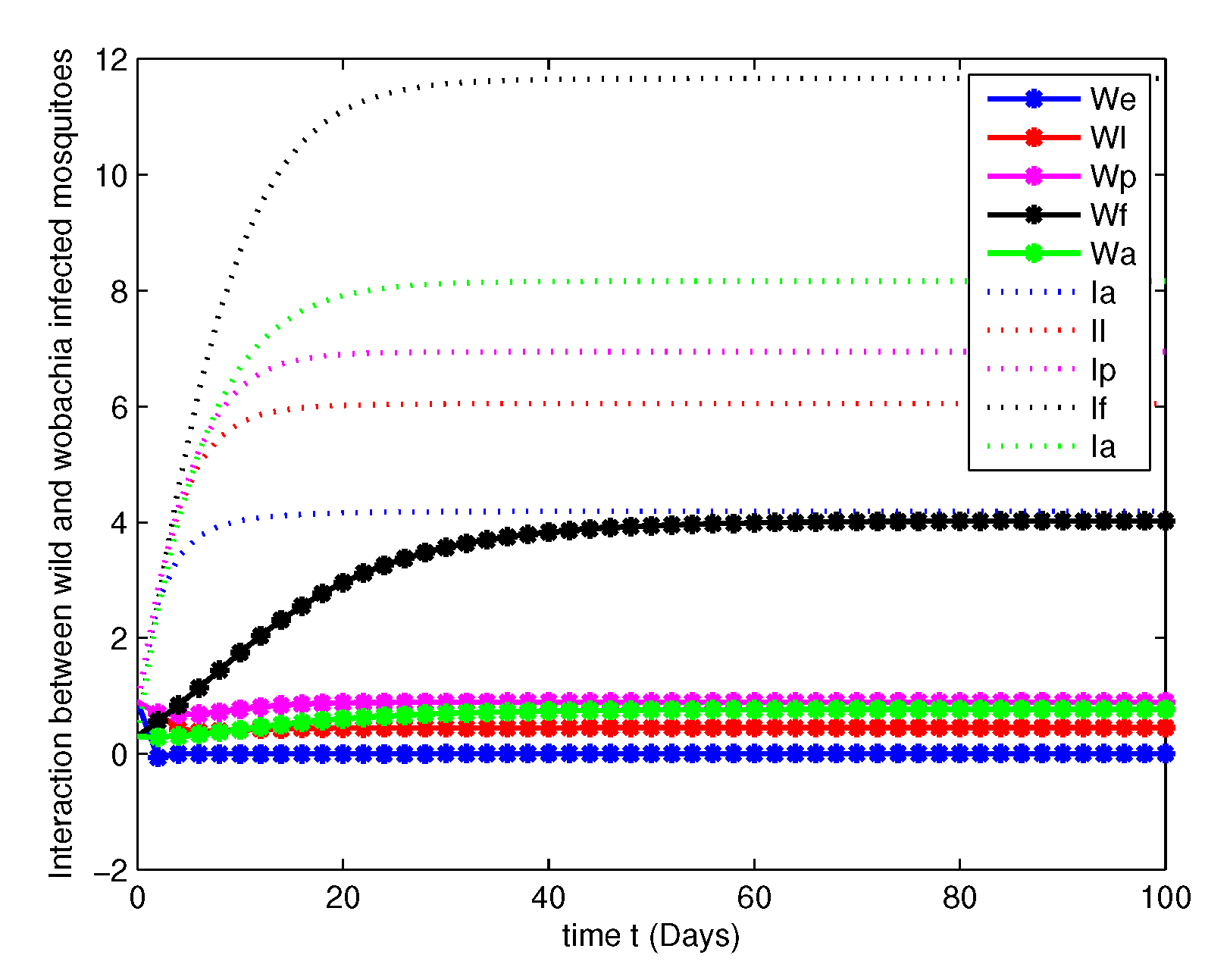
In this section, we provide an example to show the benefits of the proposed models (5)–(7). In this, we have analyzed three cases by published data mentioned in Table 2.
Case 1.
In this case, we have analyzed the transmission dynamics of Wolbachia among Aedes Aegypti mosquitoes via substituting the values mentioned in Table 2.
For this consider the system (5), with initial conditions W e 0 = 0.9 , W l 0 = 0.9 , W p 0 = 0.9 , W f 0 = 0.3 , W a 0 = 0.3 , I e 0 = 0.9 , I l 0 = 0.9 , I p 0 = 0.9 , I f 0 = 0.3 , I a 0 = 0.3 , total population T = 3000 , and the positive scalar used in Theorem 2 as ξ = 0.8513
The Figure 4, Figure 5, Figure 6 and Figure 7 are depicts the dynamics of Equation (5) along with the parameters in Table 2 at various orders of α such as α = 0.28 , 0.68 , 0.98 and 1. We can observe by simulation results that, there is a notable decrease in non-Wolbachia mosquitoes and increase in Wolbachia infected mosquitoes.
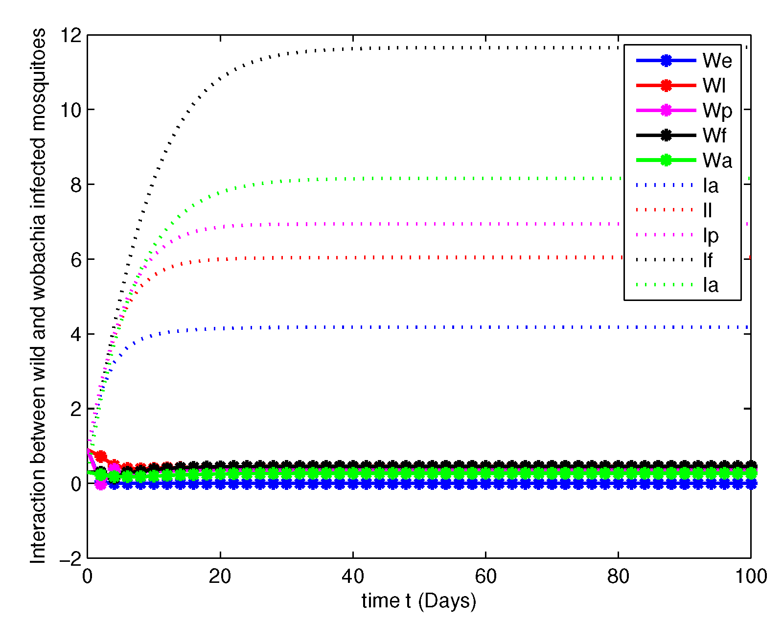
Case 2.
In this case, we have analyzed the merits and demerits of considering the Wolbachia invasion. For this consider the system of Equation (6) with parameters mentioned in Table 2. We have plotted (6) with initial conditions and total population as considered in Case 1. Along with this, the other parameters η 1 = 0.03 , η 2 = 0.03 , η 3 = 0.03 , η 4 = 0.5 and η 1 = 0.5 are fitted.
Figure 8, Figure 9, Figure 10 and Figure 11 are analyzed the dynamics of the system of Equation (6), with Wolbachia invasion and natural Wolbachia gain at various orders α = 0.28 , 0.68 , 0.98 and 1. From this we can observe that, Wolbachia infected mosquitoes tends to annihilation before the eradication of non-Wolbachia mosquitoes. It will lead to the decay in natural CI rescue.
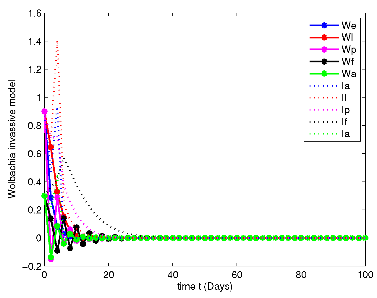
Case 3.
In this case, the decay due to the natural Wolbachia invasion is managed by releasing Wolbachia infected mosquitoes impulsively. For this case, along with the parameters mentioned in Table 2, we have fitted the values of impulsive control as δ 1 = 0.4 , δ 2 = 0.4 , δ 3 = 0.3 , δ 4 = 0.5 and δ 5 = 0.5 , invasion rates are η 1 = 0.03 , η 2 = 0.03 , η 3 = 0.03 , and gain rates are η 4 = 0.5 and η 1 = 0.5 .
Figure 12, Figure 13, Figure 14 and Figure 15 explicitly shows the dynamics of the systems of Equation (7) with impulsive control at orders α = 0.28 , 0.68 , 0.98 and 1. From this we get that, at order α = 0.28 the system leads to instability, when α = 0.68 the system started to posses stable state and at α = 1 the both population are annihilated at initial stage compared with Figure 7 and Figure 11.
By observing all the three cases, we can conclude that an impulsive control is an effective control strategy at Wolbachia invasion environment.

9. Conclusions

The effect of Wolbachia invasion and gain in vector population can lead to non-negligible in disease prevalence. Our impulsive control strategy shows that it is possible to control the transmission and invasion dynamics of Wolbachia bacterium. Our results shows that this method will increase the self-sustainability of Wolbachia bacterium among Aedes Aegypti mosquitoes. Another key result of the proposed fractional order model is, both mosquitoes population tends to annihilation after an impulsive controller synthesis. Further works on this model such as linearization, Lyapunov construction depicts that the created mathematical model is global Mittag-Leffler stable. In simulation performed here, depicts the effectiveness of the proposed model. In thus, we incorporated the real-world data from existing literature to compare the dynamical simulation of the 3 cases of model such as in the absence of Wolbachia invasion, the presence of Wolbachia invasion and the presence of Wolbachia invasion along with the impulsive control.

Author Contributions

Conceptualization, J.D. and R.R.; methodology, J.D. and R.R.; software, J.D. and R.R.; validation, J.D., R.R., J.A., M.N. and O.B.; formal analysis, J.D. and R.R.; investigation, J.D. and R.R.; resources, J.D. and R.R.; data curation, J.D. and R.R.; writing—original draft preparation, J.D. and R.R.; writing—review and editing, J.D. and R.R.; visualization, J.D., R.R., J.A., M.N. and O.B.; supervision, R.R., J.A., M.N. and O.B.; project administration, J.D. and R.R.; funding acquisition, J.A. All authors have read and agreed to the published version of the manuscript.

Funding

J. Alzabut would like to thank Prince Sultan University for supporting and funding this work through research group Nonlinear Analysis Methods in Applied Mathematics (NAMAM) group number RG-DES-2017-01.

Institutional Review Board Statement

Not applicable.

Informed Consent Statement

Not applicable.

Data Availability Statement

Not applicable.

Acknowledgments

This article has been written with the joint partial financial support of SERB-EEQ/2019/000365, the National Science Centre in Poland Grant DEC-2017/25/ B/ST7/02888, RUSA Phase 2.0 Grant No. F 24–51/2014-U, Policy (TN Multi-Gen), Dept.of Edn. Govt. of India, UGC-SAP (DRS-I) Grant No. F.510/8/DRS-I/ 2016(SAP-I), DST-PURSE 2nd Phase programme vide letter No. SR/ PURSE Phase 2/38 (G), DST (FIST - level I) 657876570 Grant No.SR/FIST/MS-I/ 2018/17.

Conflicts of Interest

The authors declare no conflict of interest.

Appendix A

Appendix A.1. Wolbachia Infected Mosquitoes Free Equilibrium

Suppose, there is no Wolbachia infected mosquitoes population then the possible equilibrium can be written as
P 2 = ( W e 1 * , W l 1 * , W p 1 * , W f 1 * , W a 1 * , 0 , 0 , 0 , 0 , 0 )
where,
W e 1 * = T λ w f λ w a ( λ w e + γ w e ) ( λ w l + γ w l ) 2 ( λ w p + γ w p ) 2 ρ ( 1 ρ ) Λ w e γ w p 2 γ w e 2 γ w l 2 W l 1 * = γ w e λ w l + γ w l W e 1 * W p 1 * = γ w l γ w e ( λ w l + γ w l ) ( λ w p + γ w p ) W e 1 * W f 1 * = ρ γ w p γ w e γ w l λ w f ( λ w f + γ w f ) ( λ w p + γ w p ) W e 1 * W a 1 * = ( 1 ρ ) γ w p γ w e λ w e ( λ w l + γ w l ) ( λ w p + γ w p ) W e 1 *
These equilibrium points were derived by the following system of equations by putting I e 1 * = 0 , I l 1 * = 0 , I p 1 * = 0 , I f 1 * = 0 , I a 1 * = 0 .
That is,
Λ w e W f 1 * W a 1 * T λ w e W e 1 * γ w e W e 1 * = 0 γ w e W e 1 * λ w l W l 1 * γ w l W l 1 * + ( 1 α ) γ i e I e 1 * = 0 γ w l W l 1 * λ w p W p 1 * γ w p W p 1 * + ( 1 β ) γ i l I l 1 * = 0 ρ γ w p W p 1 * λ w f W f 1 * + ( 1 ϵ ) γ i p ρ i w I p 1 * = 0 ( 1 ρ ) γ w p W p 1 * λ w a W a 1 * + ( 1 ϵ ) γ i p ( 1 ρ i w ) I p 1 * = 0
That is,
(i).
By solving,
γ w e W e 1 * λ w l W l 1 * γ w l W l 1 * + ( 1 α ) γ i e I e 1 * = 0
We get the value of W l * as,
W l * = γ w e ( λ w l + γ w l ) W e *
(ii).
By solving
γ w l W l 1 * λ w p W p 1 * γ w p W p 1 * + ( 1 β ) γ i l I l 1 * = 0
We get the value of W p * as,
W p * = γ w l λ w p + γ w p W l *
Substitute the value of W l * from (i),
W p * = γ w l γ w e ( λ w p + γ w p ) ( λ w l + γ w l ) W e *
(iii).
By solving
ρ γ w p W p 1 * λ w f W f 1 * + ( 1 ϵ ) γ i p ρ i w I p 1 * = 0
We get the value of W f * as,
W f * = ρ γ w p λ w f W p *
Substitute the value of W p * from (ii),
W f * = ρ γ w p γ w e γ w l λ w f ( λ w p + γ w p ) ( λ w l + γ w l ) W e *
(iv).
By solving
( 1 ρ ) γ w p W p 1 * λ w a W a 1 * + ( 1 ϵ ) γ i p ( 1 ρ i w ) I p 1 * = 0
We get the value of W a * as,
W a * = ( 1 ρ ) γ w p λ w a W p *
Substitute the value of W p * from (ii),
W a * = ( 1 ρ ) γ w p γ w l γ w e λ w a ( λ w l + γ w l ) ( λ w p + γ w p ) W e *
(v).
By solving
Λ w e W f 1 * W a 1 * T λ w e W e 1 * γ w e W e 1 * = 0
We get the value of W e * as,
W e * = Λ w e T ( λ w e + γ w e ) W f * W a *
Substitute the value of W f * and W a * from (iii) and (iv),
W e * = T λ w f λ w a ( λ w e + γ w e ) ( λ w l + γ w l ) 2 ( λ w p + γ w p ) 2 ρ ( 1 ρ ) Λ w e γ w p 2 γ w e 2 γ w l 2

Appendix A.2. Wild Mosquitoes Free Equilibrium

Suppose a successful release of Wolbachia infected mosquitoes replaces the wild mosquitoes by Wolbachia infected mosquitoes. Then the possible equilibrium points can be found by substituting W e 2 * = 0 , W l 2 * = 0 , W p 2 * = 0 , W f 2 * = 0 and W a 2 * = 0 in the following system of equations
0 = Λ i e I f 2 * ( W a 2 * + I a 2 * ) T λ i e I e 2 * α γ i e I e 2 * 0 = α γ i e I e 2 * λ i l I l 2 * β γ i l I l 2 * 0 = β γ i l I l 2 * λ i p I p 2 * ϵ γ i p I p 2 * 0 = ρ i ϵ γ i p I p 2 * λ i f I f 2 * 0 = ( 1 ρ i ) ϵ γ i p I p 2 * λ i a I a 2 * .
(i)
By solving
0 = ( 1 ρ i ) ϵ γ i p I p 2 * λ i a I a 2 *
We get,
I a 2 * = ( 1 ρ i ) ϵ γ i p λ i a I p 2 *
(ii)
By solving
0 = ρ i ϵ γ i p I p 2 * λ i f I f 2 *
We get,
I f 2 * = ρ i ϵ γ i p λ i f I p 2 *
(iii)
By solving
β γ i l I l 2 * λ i p I p 2 * ϵ γ i p I p 2 *
We get,
I l 2 * = ( λ i p + ϵ γ i p ) β γ i l I p 2 *
(iv)
By solving
0 = α γ i e I e 2 * λ i l I l 2 * β γ i l I l 2 *
We get,
I e 2 * = ( λ i l + β γ i l ) α γ i e I l 2 *
Substitute the value of I l 2 * from (iii),
I e 2 * = ( λ i l + β γ i l ) ( λ i p + ϵ γ i p ) α β γ i e γ i l I p 2 *
(v)
By solving,
0 = Λ i e I f 2 * ( W a 2 * + I a 2 * ) T λ i e I e 2 * α γ i e I e 2 *
Put W a 2 * = 0 ,
Λ i e I f 2 * I a 2 * T λ i e I e 2 * α γ i e I e 2 * = 0 Λ i e T ρ i ϵ γ i p λ i f I p 2 * ( 1 ρ i ) ϵ γ i p λ i a I p 2 * = ( λ i e + α γ i e ) I e 2 * I p 2 * = T λ i f λ i a ( λ i e + α γ i e ) ( λ i l + β γ i l ) ( λ i p + ϵ γ i p ) Λ i e α β ρ i ( 1 ρ i ) ϵ 2 γ i p 2 γ i e γ i l
From (i)–(v) we have the following equilibrium point,
P 3 = ( 0 , 0 , 0 , 0 , 0 , I e 2 * , I l 2 * , I p 2 * , I f 2 * , I a 2 * )
where,
I e 2 * = ( λ i l + β γ i l ) ( λ i p + ϵ γ i p ) α β γ i e γ i l I p 2 * I l 2 * = ( λ i p + ϵ γ i p ) β γ i l I p 2 * I p 2 * = T λ i f λ i a ( λ i e + α γ i e ) ( λ i l + β γ i l ) ( λ i p + ϵ γ i p ) Λ i e α β ρ i ( 1 ρ i ) ϵ 2 γ i p 2 γ i e γ i l I f 2 * = ρ i ϵ γ i p λ i f I p 2 * I a 2 * = ( 1 ρ i ) ϵ γ i p λ i a I p 2 *

Appendix A.3. Both Wolbachia and Non-Wolbachia Mosquitoes Co-Existence Equilibrium

The equilibrium point for the co-existence state can be found by solving the following systems of equations
Λ w e n W f n * W a n * T λ w e W e n * γ w e W e n * = 0 γ w e W e n * λ w l W l n * γ w l W l n * + ( 1 α ) γ i e I e n * = 0 γ w l W l n * λ w p W p n * γ w p W p n * + ( 1 β ) γ i l I l n * = 0 ρ γ w p W p n * λ w f W f n * + ( 1 ϵ ) γ i p ρ i w I p n * = 0 ( 1 ρ ) γ w p W p n * λ w a W a n * + ( 1 ϵ ) γ i p ( 1 ρ i w ) I p n * = 0 Λ i e I f n * ( W a n * + I a n * ) T λ i e I e n * α γ i e I e n * = 0 α γ i e I e n * λ i l I l n * β γ i l I l n * = 0 β γ i l I l n * λ i p I p n * ϵ γ i p I p n * = 0 ρ i ϵ γ i p I p n * λ i f I f n * = 0 ( 1 ρ i ) ϵ γ i p I p n * λ i a I a n * = 0 .
(i)
( 1 ρ i ) ε γ i p I p n * λ i a I a n * = 0 I p n * = λ i a ( 1 ρ i ) ε γ i p I a n *
(ii)
ρ i ε γ i p I p n * λ i f I f n * = 0 I f n * = ρ i ε γ i p λ i f I p n * I f n * = ρ i λ i a ( 1 ρ i ) λ i f I a n *
(iii)
β γ i l I l n * λ i p I p n * ε γ i p I p n * = 0 I l n * = λ i a β γ i l ( 1 ρ i ) 1 + λ i p ε γ i p I a n *
Let B 1 = 1 + λ i p ε γ i p
I l n * = λ i a B 1 β γ i l ( 1 ρ i ) I a n *
(iv)
α γ i e I e n * λ i l I l n * β γ i l I l n * = 0 I e n * = ( λ i l + β γ i l ) α γ i e I l n * I e n * = B 1 B 2 λ i a α γ i e ( 1 ρ i ) I a n *
Where, B 1 = 1 + λ i p ε γ i p ; B 2 = 1 + λ i l β γ i l
(v)
Λ I e n I f n * W a n * + Λ I e n I f n * I a n * T λ i e I e n * α γ i e I e n * = 0 W a n * = T ( λ i e + α γ i e ) Λ i e I f n * I e n * I a n * W a n * = T B 1 B 2 λ i f ( λ i e + α γ i e ) α Λ i e ρ i γ i e I a n * W a n * = T B 1 B 2 B 3 λ i f ρ i Λ i e I a n *
Where, B 3 = 1 + λ i e α γ i e
(vi)
( 1 ρ ) γ w p W p n * λ w a W a n * + ( 1 ε ) γ i p ( 1 ρ i w ) I p n * = 0 W p n * = λ w a ( 1 ρ ) γ w p W a n * ( 1 ε ) γ i p ( 1 ρ i w ) ( 1 ρ ) γ w p I p n * W p n * = T B 1 B 2 B 3 λ i f λ w a Λ i e ( 1 ρ ) ρ i γ w p B 4 I a n *
where, B 4 = 1 + ( 1 ε ) ( 1 ρ i w ) λ i a ( 1 ρ ) ( 1 ρ i ) ε γ w p
(vii)
ρ γ w p W p n * λ w f W f n * + ( 1 ε ) γ i p ρ i w I p n * = 0 W f * = ρ γ w p λ w f T B 1 B 2 B 3 λ i f λ w a Λ i e ( 1 ρ ) ρ i γ w p B 4 I a n * + ( 1 ε ) ρ i w λ i a ε λ w f ( 1 ρ i ) I a n *
(viii)
γ w l W l n * λ w p W p n * γ w p W p n * + ( 1 β ) γ i l I l n * = 0 W l n * = λ w p + γ w p γ w l W p n * ( 1 β ) γ i l γ w l I l n * W l n * = λ w p + γ w p γ w l T B 1 B 2 B 3 λ i f λ w a Λ i e ( 1 ρ ) ρ i γ w p B 4 I a n * ( 1 β ) γ i l γ w l λ i a B 1 β γ i l ( 1 ρ i ) I a n *
(ix)
γ w e W e n * λ w l W l n * γ w l W l n * + ( 1 α ) γ i e I e n * = 0 W e n * = λ w l + γ w l γ w e W l n * ( 1 α ) γ i e γ w e I e n * W e n * = λ w l + γ w l γ w e λ w p + γ w p γ w l T B 1 B 2 B 3 λ i f λ w a Λ i e ( 1 ρ ) ρ i γ w p I a n * γ w e [ B 4 ( λ w l + γ w l ) λ w p + γ w p γ w l + λ w l + γ w l ( 1 β ) γ i l γ w l λ i a B 1 β γ i l ( 1 ρ i ) + ( 1 α ) γ i e λ i a B 1 B 2 α γ i e ( 1 ρ i ) ]
(x)
Λ w e W f * W a * T λ w e W e * γ w e W e * = 0 W f * W a * Λ w e T = Λ w e ρ B 4 γ w p T λ w f ( I a * ) 2 Λ w e ρ B 1 B 2 B 3 λ i f ρ i Λ I e λ w f × λ w a ( 1 ρ ) + B 4 γ w p I a * + Λ w e ρ B 1 2 B 2 2 B 3 2 λ i f 2 λ w e Λ I e 2 ( 1 ρ ) ρ i 2 λ w f ( λ w e + γ w e ) W e * = λ w e + γ w e λ w p + γ w p λ w l + γ w l γ w e γ w l λ w e + γ w e γ w e × [ λ w p + γ w p λ w l + γ w l B 4 γ w l + λ w l + γ w l ( 1 β ) λ i a B 1 γ w l β ( 1 ρ i ) + ( 1 α ) λ i a B 1 B 2 α ( 1 ρ i ) ] I a * Λ w e W f * W a * T λ w e W e * γ w e W e * = 0 Λ w e ρ B 4 γ w p T λ w f ( I a * ) 2 λ w e + γ w e γ w e Λ w e ρ B 1 B 2 B 3 λ f * ρ i Λ I e λ w f λ w a ( 1 ρ ) + B 4 γ w p × [ λ w p + γ w p λ w l + γ w l B 4 γ w l + λ w l + γ w l ( 1 β ) λ i a B 1 γ w l β ( 1 ρ i ) + ( 1 α ) λ i a B 1 B 2 α ( 1 ρ i ) ] I a * + Λ w e ρ B 1 2 B 2 2 B 3 2 λ i f 2 λ w e Λ I e 2 ( 1 ρ ) ρ i 2 λ w f = 0
The above equation is a quadratic equation on I a n * . That is,
a 1 I a n * 2 + a 2 I a n * + a 3 = 0 ,
where,
a 1 = Λ w e ρ B 4 γ w p T λ w f ; a 2 = λ w e + γ w e T λ w f λ w e λ i f ρ B 1 B 2 B 3 ρ i Λ i e λ w f λ w a ( 1 ρ ) + B 4 γ w p ( λ w l + γ w l ) ( λ w p + γ w p ) B 4 γ w l + ( λ w l + γ w l ) ( 1 β ) λ i a B 1 γ w l β ( 1 ρ i ) + ( 1 α ) λ i a B 1 B 2 α ( 1 ρ i ) ; a 3 = Λ w e ρ T B 1 2 B 2 2 B 3 2 λ w a Λ i e 2 ( 1 ρ ) ρ i 2 λ w f .
These are the equilibrium points presented in Section 4.4.

References

  1. kilbas, A.A.; Sirvastava, H.M.; Trujillo, J.J. Theory and Applications of Fractional Differential Equations; Elsevier: Amsterdam, The Netherlands, 2006. [Google Scholar]
  2. Rahimy, M. Applications of fractional differential equations. Appl. Math. Sci. 2010, 4, 2453–2461. [Google Scholar]
  3. Samko, S.G.; Kilbas, A.A.; Marichev, O.I. Fractional Integrals and Derivatives: Theory and Applications; Gordon & Breach, Science Publications: London, UK; New York, NY, USA, 1993. [Google Scholar]
  4. Podlubny, I. Fractional Differential Equations: An Introduction to Fractional Derivatives, Fractional Differential Equations, to Methods of Their Solution and Some of Their Applications; Academic Press: Cambridge, MA, USA, 1999. [Google Scholar]
  5. Podlubny, I. Geometric and physical interpretation of fractional integration and fractional differentiation. Fract. Calc. Appl. Anal. 2002, 5, 367–386. [Google Scholar]
  6. Oldham, K.B.; Spanier, J. The Fractional Calculus; Academic Press: New York, NY, USA; London, UK, 1974. [Google Scholar]
  7. Li, Y.; Chen, Y.; Podlubny, I. Stability of fractional-order nonlinear dynamic systems: Lyapunov direct method and generalized Mittag-Leffler stability. Comput. Math. Appl. 2010, 59, 1810–1821. [Google Scholar] [CrossRef] [Green Version]
  8. Gibbons, R.; Vaughn, D. Dengue: An escalating problem. BMJ 2002, 324, 1563–1566. [Google Scholar] [CrossRef] [PubMed] [Green Version]
  9. Bhatt, S.; Gething, P.W.; Brady, O.J.; Messina, J.P.; Farlow, A.W.; Moyes, C.L.; Drake, J.M.; Brownstein, J.S.; Hoen, A.G.; Sankoh, O.; et al. The global distribution and burden of dengue. Nature 2013, 496, 504–507. [Google Scholar] [CrossRef] [PubMed]
  10. Chye, J.K.; Lim, C.T.; Ng, K.B. Vertical transmission of dengue. Clin. Infect. Dis. 1997, 25, 1374–1377. [Google Scholar] [CrossRef] [PubMed] [Green Version]
  11. Kraemer, M.; Sinka, M.; Duda, K.; Mylne, A.; Shearer, F.; Barker, C. The global distribution of the arbovirus vectors Aedes aegypti and Ae. albopictus. eLife 2015, 4, 1–18. [Google Scholar] [CrossRef]
  12. Gubler, D.J. Dengue and dengue hemorrhagic fever. Clin. Microbiol. Rev. 1998, 11, 480–496. [Google Scholar] [CrossRef] [Green Version]
  13. Gubler, D.J. Epidemic dengue/dengue hemorrhagic fever as a public health, social and economic problem in the 21st century. Trends Microbiol. 2002, 10, 100–103. [Google Scholar] [CrossRef]
  14. Ong, A.; Sandar, M.; Chen, M.I.; Sin, L.Y. Fatal dengue hemorrhagic fever in adults during a dengue epidemic in Singapore. Int. J. Infect. Dis. 2007, 11, 263–267. [Google Scholar] [CrossRef] [Green Version]
  15. World Health Organization. Vector-Borne Diseases. 2020. Available online: http://www.who.int/mediacentre/factsheets/fs387/en/ (accessed on 25 January 2021).
  16. Alphey, L.; Benedict, M.; Bellini, R.; Clark, G.G.; Dame, D.A.; Service, M.W.; Dobson, S.L. Sterile-insect methods for control of mosquito-borne diseases: An analysis. Vector-Borne Zoonotic Dis. 2010, 10, 295–311. [Google Scholar] [CrossRef] [PubMed]
  17. Bouyer, J.; Lefrancois, T. Boosting the sterile insect technique to control mosquitoes. Trends Parasitol. 2014, 30, 271–273. [Google Scholar] [CrossRef] [PubMed]
  18. Fu, G.; Lees, R.S.; Nimmo, D.; Aw, D.; Jin, L.; Gray, P.; Berendonk, T.U. Femalespecific flightless phenotype for mosquito control. Proc. Natl. Acad. Sci. USA 2010, 107, 4550–4554. [Google Scholar] [CrossRef] [Green Version]
  19. James, A.A. Gene drive systems in mosquitoes: Rules of the road. Trends Parasitol. 2005, 21, 64–67. [Google Scholar] [CrossRef]
  20. Scott, T.W.; Takken, W.; Knols, B.G.J.; Boëte, C. The ecology of genetically modified mosquitoes. Science 2002, 298, 117–119. [Google Scholar] [CrossRef] [PubMed]
  21. Masud, M.A.; Kim, B.N.; Kim, Y. Optimal control problems of mosquito-borne disease subject to changes in feeding behaviour of Aedes mosquitoes. Biosystems 2017, 156–157, 23–39. [Google Scholar] [CrossRef]
  22. Momoh, A.A.; Fugenschuh, A. Optimal control of intervention strategies and cost effectiveness analysis for a zika virus model. Oper. Res. Health Care 2018, 18, 99–111. [Google Scholar] [CrossRef]
  23. Segoli, M.; Hoffmann, A.A.; Lloyd, J.; Omodei, G.J.; Ritchie, S.A. The effect of virus-blocking Wolbachia on male competitiveness of the dengue vector mosquito, Aedes aegypti. PLOS Negl. Trop. Dis. 2014, 8, e3294. [Google Scholar] [CrossRef] [PubMed]
  24. Walker, T.; Johnson, P.H.; Moreira, L.A.; Iturbe-Ormaetxe, I.; Frentiu, F.D.; McMeniman, C.J.; Leong, Y.S.; Dong, Y.; Axford, J.; Kriesner, P.; et al. The WMel Wolbachia strain blocks dengue and invades caged Aedes aegypti populations. Nature 2011, 476, 450–453. [Google Scholar] [CrossRef]
  25. Xi, Z.; Khoo, C.C.; Dobson, S.L. Wolbachia establishment and invasion in an Aedes aegypti laboratory population. Science 2005, 310, 326–328. [Google Scholar] [CrossRef] [Green Version]
  26. Ormaetxe, I.; Walker, T.; Neill, S.L.O. Wolbachia and the biological control of mosquito-borne disease. Embo Rep. 2011, 12, 508–518. [Google Scholar] [CrossRef] [Green Version]
  27. World Mosquito Program. Available online: https://www.worldmosquitoprogram.org (accessed on 25 January 2021).
  28. Dutra, H.L.C.; Rocha, M.N.; Dias, F.B.S.; Mansur, S.B.; Caragata, E.P.; Moreira, L.A. Wolbachia blocks currently circulating Zika virus isolates in Brazilian Aedes aegypti mosquitoes. Cell Host Microbe 2016, 19, 771–774. [Google Scholar] [CrossRef] [PubMed] [Green Version]
  29. Hancock, P.; Sinkins, S.; Godfray, H. Population dynamic models of the spread of Wolbachia. Am. Nat. 2011, 177, 323–333. [Google Scholar] [CrossRef] [Green Version]
  30. Hughes, H.; Britton, N. Modelling the use of Wolbachia to control dengue fever transmission. Bull. Math. Biol. 2013, 75, 796–818. [Google Scholar] [CrossRef] [Green Version]
  31. McMeniman, C.J.; Lane, R.V.; Cass, B.N.; Fong, A.W.; Sidhu, M.; Wang, Y.F.; Neill, S.L.O. Stable introduction of a life-shortening Wolbachia infection into the mosquito Aedes aegypti. Science 2009, 323, 141–144. [Google Scholar] [CrossRef] [Green Version]
  32. Jiggins, F. The spread of Wolbachia through mosquito populations. PLoS Biol. 2017, 15, e2002780. [Google Scholar] [CrossRef]
  33. Ndii, M.Z.; Hickson, R.I.; Allingham, D.; Mercer, G.N. Modelling the transmission dynamics of dengue in the presence of Wolbachia. Math. Biosci. 2015, 262, 157–166. [Google Scholar] [CrossRef]
  34. Koiller, J.; da Silva, M.A.; Souza, M.O.; Codeco, C.; Iggidr, A.; Sallet, G. Aedes, Wolbachia and Dengue; Inria Nancy-Grand Est: Villers-lès-Nancy, France, 2014; pp. 1–47. [Google Scholar]
  35. Adekunle, A.I.; Michael, M.T.; McBryde, E.S. Mathematical analysis of a Wolbachia invasive model with imperfect maternal transmission and loss of Wolbachia infection. Infect. Dis. Model. 2019, 4, 265–285. [Google Scholar] [CrossRef]
  36. Xue, L.; Manore, C.; Thongsripong, P.; Hyman, J. Two-sex mosquito model for the persistence of Wolbachia. J. Biol. Dyn. 2017, 11, 216–237. [Google Scholar] [CrossRef] [Green Version]
  37. Rock, K.S.; Wooda, D.A.; Keeling, M.J. Age- and bite-structured models for vector-borne diseases. Epidemics 2015, 12, 20–29. [Google Scholar] [CrossRef] [PubMed] [Green Version]
  38. Rafikov, M.; Meza, M.E.M.; Correa, D.P.F.; Wyse, A.P. Controlling Aedes aegypti populations by limited Wolbachia-based strategies in a seasonal environment. Math. Methods Appl. Sci. 2019, 42, 5736–5745. [Google Scholar] [CrossRef]
  39. Supriatna, A.K.; Anggriani, N.; Melanie; Husniah, H. The optimal strategy of Wolbachia- infected mosquitoes release program an application of control theory in controlling Dengue disease. In Proceedings of the 2016 International Conference on Instrumentation, Control and Automation(ICA), Bandung, Indonesia, 29–31 August 2016; pp. 38–43. [Google Scholar]
  40. Dianavinnarasi, J.; Cao, Y.; Raja, R.; Rajchakit, G.; Lim, C.P. Delay-dependent stability criteria of delayed positive systems with uncertain control inputs: Application in mosquito-borne morbidities control. Appl. Math. Comput. 2020, 382, 125210. [Google Scholar] [CrossRef]
  41. Dianavinnarasi, J.; Raja, R.; Alzabut, J.; Cao, J.; Niezabitowski, M.; Bagdasar, O. Application of Caputo—Fabrizio operator to suppress the Aedes Aegypti mosquitoes via Wolbachia: An LMI approach. Math. Comput. Simul. 2021. [Google Scholar] [CrossRef]
  42. Nisar, K.S.; Ahmad, S.; Ullah, A.; Shah, K.; Alrabaiah, H.; Arfan, M. Mathematical analysis of SIRD model of COVID-19 with Caputo fractional derivative based on real data. Results Phys. 2021, 21, 103772. [Google Scholar] [CrossRef]
  43. Boyd, S.; Ghaoui, L.; Feron, E.; Balakrishnan, V. Linear Matrix Inequalities in System and Control Theory; SIAM Philadelphia: Philadelphia, PA, USA, 1994. [Google Scholar]
  44. Wu, H.; Zhang, X.; Xue, S.; Wang, L.; Wang, Y. LMI conditions to global Mittag-Leffler stability of fractional-order neural networks with impulses. Neurocomputing 2016, 193, 148–154. [Google Scholar] [CrossRef]
  45. Stamova, I. Global stability of impulsive fractional differential equations. Appl. Math. Comput. 2014, 237, 605–612. [Google Scholar] [CrossRef]
  46. Agarwal, R.P.; Meehan, M.; O’Regan, D. Fixed Point Theory and Applications; Cambridge University Press: Cambridge, UK, 2001. [Google Scholar]
  47. Iswarya, M.; Raja, R.; Rajchakit, G.; Alzabut, J.; Lim, C.P. A perspective on graph theory based stability analysis of impulsive stochastic recurrent neural networks with time-varying delays. Adv. Differ. Equ. 2019, 502, 1–21. [Google Scholar] [CrossRef] [Green Version]
  48. Stamov, G.; Stamova, I.; Alzabut, J. Global exponential stability for a class of impulsive BAM neural networks with distributed delays. Appl. Math. Inf. Sci. 2013, 7, 1539–1546. [Google Scholar] [CrossRef]
  49. Stamov, G.T.; Alzabut, J.O.; Atanasov, P.; Stamov, A.G. Almost periodic solutions for impulsive delay model of price fluctuations in commodity markets. Nonlinear Anal. Real World Appl. 2011, 12, 3170–3176. [Google Scholar] [CrossRef]
  50. Zada, A.; Waheed, H.; Alzabut, J.; Wang, X. Existence and stability of impulsive coupled system of fractional integrodifferential equations. Demonstr. Math. 2019, 52, 296–335. [Google Scholar] [CrossRef]
  51. Zada, A.; Alam, L.; Kumam, P.; Kumam, W.; Ali, G.; Alzabut, J. Controllability of impulsive non-linear delay dynamic systems on time scale. IEEE Access 2020, 8, 93830–93839. [Google Scholar] [CrossRef]
  52. Ndii, M.Z.; Hickson, R.I.; Mercer, G.N. Modelling the introduction of Wolbachia into Aedes aegypti to reduce dengue transmission. Anziam J. 2012, 53, 213–227. [Google Scholar]
  53. Yang, H.M.; Macoris, M.L.G.; Galvani, K.C.; Andrighetti, M.T.M.; Wanderley, D.M.V. Assessing the effects of temperature on the population of Aedes aegypti, the vector of dengue. Epidemiol. Infect. 2009, 137, 1188–1202. [Google Scholar] [CrossRef] [PubMed] [Green Version]
  54. Maidana, N.A.; Yang, H.M. Describing the geographic spread of dengue disease by traveling waves. Math. Biosci. 2008, 215, 64–77. [Google Scholar] [CrossRef]
Figure 1. Mechanism of Wolbachia among mosquitoes and human.
Symmetry 13 00434 g001
Figure 2. Block diagram representing the mechanism of Wolbachia infection in mosquitoes.
Symmetry 13 00434 g002
Figure 3. Schematic representation Wolbachia spread dynamics among Aedes Aegypti mosquitoes.
Symmetry 13 00434 g003
Figure 4. Population dynamics of both WU and WI mosquitoes at α = 0.28 .
Symmetry 13 00434 g004
Figure 5. Population dynamics of both WU and WI mosquitoes at α = 0.68 .
Symmetry 13 00434 g005
Figure 6. Population dynamics of both WU and WI mosquitoes at α = 0.98 .
Symmetry 13 00434 g006
Figure 7. Population dynamics of both WU and WI mosquitoes at α = 1 .
Symmetry 13 00434 g007
Figure 8. Population dynamics of Wolbachia invasive model at α = 0.28 .
Symmetry 13 00434 g008
Figure 9. Population dynamics of Wolbachia invasive model at α = 0.68 .
Symmetry 13 00434 g009
Figure 10. Population dynamics of Wolbachia invasive model at α = 0.98 .
Symmetry 13 00434 g010
Figure 11. Population dynamics of Wolbachia invasive model at α = 0.28 .
Symmetry 13 00434 g011
Figure 12. Population dynamics of Wolbachia invasive model after impulsive control at α = 0.28 .
Symmetry 13 00434 g012
Figure 13. Population dynamics of Wolbachia invasive model after impulsive control at α = 0.68 .
Symmetry 13 00434 g013
Figure 14. Population dynamics of Wolbachia invasive model after impulsive control at α = 0.98 .
Symmetry 13 00434 g014
Figure 15. Population dynamics of Wolbachia invasive model after impulsive control at α = 1 .
Symmetry 13 00434 g015
Table 1. Description of parameters involved in system of Equation (5).
ParameterDescription
Λ w e , Λ i e Reproduction rate of non-Wolbachia mosquitoes
and Wolbachia infected mosquitoes respectively
λ w e The natural death rate of eggs without Wolbachia infection
λ w l The natural death of larvae without Wolbachia infection
λ w p The natural death of pupae without Wolbachia infection
λ w f The natural death of adult female mosquitoes without Wolbachia infection
λ w a The natural death of adult male mosquitoes without Wolbachia infection
λ i e The natural death of eggs with Wolbachia infection
λ i l The natural death of larvae with Wolbachia infection
λ i p The natural death of pupae with Wolbachia infection
λ i f The natural death of adult female mosquitoes with Wolbachia infection
λ i a The natural death of infected adult male mosquitoes with Wolbachia infection
γ w e The rate at which the fraction of non-Wolbachia eggs matured into non-Wolbachia larvae
γ w l The rate at which the fraction of non-Wolbachia larvae matured into non-Wolbachia pupae
γ w p The rate at which the fraction of non-Wolbachia pupae matured into non-Wolbachia
immature female or male
γ i e The rate at which the fraction of the Wolbachia infected mosquito eggs
matured into Wolbachia infected or uninfected larvae
γ i l The rate at which the fraction of the Wolbachia infected mosquito larvae
matured into Wolbachia infected or uninfected pupae
γ i p The rate at which the fraction of the Wolbachia infected mosquito pupae
matured into Wolbachia infected or uninfected adults
ρ The probability of having male or female mosquitoes
Table 2. Data from published literature.
ParametersDescriptionData
Λ w e Reproduction rate of Wolbachia uninfected mosquitoes1.25/day [52]
λ w e , λ w l , λ w p The death rate of aquatic Wolbachia uninfected mosquitoes 1 7.78 /day [53]
γ w e , γ w l , γ w p The Maturation rate of Wolbachia uninfected mosquitoes 1 6.67 /day [54]
λ w f , λ w a The death rate of adult Wolbachia uninfected mosquitoes 1 14 /day [53]
λ i e , λ i l , λ i p The death rate of aquatic Wolbachia infected mosquitoes 1 7.78 /day [53]
λ i f , λ i a The death rate of adult Wolbachia infected mosquitoes 1 7 /day [24]
Λ i e Reproduction rate of Wolbachia infected mosquitoes 0.95 Λ w e / d a y [52]
γ i e , γ i l , γ i p The maturation rate of Wolbachia infected mosquitoes 1 6.67 /day [24]
Publisher’s Note: MDPI stays neutral with regard to jurisdictional claims in published maps and institutional affiliations.

