Article

Feature Extraction of Marine Water Pollution Based on Data Mining

1
School of Artificial Intelligence and Big Data, Hebei Polytechnic Institute, Shijiazhuang 050091, China
2
School of Network and Communication, Hebei Polytechnic Institute, Shijiazhuang 050091, China
*
Author to whom correspondence should be addressed.
Symmetry 2021, 13(2), 355; https://doi.org/10.3390/sym13020355
Submission received: 21 January 2021 / Revised: 5 February 2021 / Accepted: 14 February 2021 / Published: 22 February 2021

Abstract

:
The ocean occupies more than two-thirds of the earth’s area, providing a lot of oxygen and materials for human survival and development. However, with human activities, a large number of sewage, plastic bags, and other wastes are discharged into the ocean, and the problem of marine water pollution has become a hot topic in the world. In order to extract the characteristics of marine water pollution, this study proposed K-means clustering technology based on cosine distance and discrimination to study the polluted water. In this study, the polygonal area method combined with six parameters of water quality is used to analyze the marine water body anomalies, so as to realize the rapid and real-time monitoring of marine water body anomalies. At the same time, the cosine distance method and discrimination are used to classify marine water pollutants, so as to improve the classification accuracy. The results show that the detection rate of water quality anomalies is more than 88.2%, and the overall classification accuracy of water pollution is 96.3%, which proves the effectiveness of the method. It is hoped that this study can provide timely and effective data support for the detection of marine water bodies.

1. Introduction

With the unprecedented prosperity of international trade since the 20th century, the marine transportation industry has been greatly developed, and the marine oil spill pollution caused by marine oil tankers is becoming more and more serious. In addition, the discharge of a large amount of wastewater and garbage aggravates the degree of marine pollution. It can be said that all marine pollution is related to human activities. However, there is a certain lag in the current water quality monitoring technology, which is very unfavorable for the timely detection of marine water pollution. With the rapid development of big data technology, online water quality monitoring technology based on data mining has begun to develop, but the related research and application are limited. Under the existing technical means, it is very important to combine the data mining technology to extract and judge the water quality monitoring information efficiently.
In this study, the conventional simple water quality parameters are used to achieve rapid detection, the six-parameter water quality model based on the polygon area method is used to achieve pollution feature extraction, and the K-means clustering analysis is used to classify the characteristics of marine water pollution. According to the blacklist of priority pollutants in water, six representative water quality parameters were selected, and a water quality parameter model was established. In the process of pollution feature classification and recognition, the idea of cluster analysis is used to transform cosine similarity into cosine distance, and the index of discrimination is proposed.
On the other hand, the traditional K-means clustering method is innovated, and the cosine distance is optimized by differentiation, which is to further improve the accuracy of marine water pollution classification and recognition.
The research is divided into four parts. The first part describes the international research progress on water quality monitoring and its application in data mining technology; the second part describes the polygon area method and clustering classification recognition method in detail; the third part shows the important results of the study and focuses on the discussion combined with the existing related research; finally, the paper discusses the current situation of water quality monitoring and its application in data mining technology The conclusion of the study is summarized, and its academic impact, limitations, and future research direction are briefly explained.

2. Related Work

2.1. Study on the Method of Water Pollution Feature Extraction

Water is an important resource for human survival. With the development of modern society, water quality monitoring has become the basic step of environmental protection, and monitoring technology innovation is the focus of environmental workers. Subbiah et al. used cyanobacteria as a key indicator to monitor water quality changes, and they studied the relationship between inorganic ion concentration and cyanobacterial toxin concentration in water, aiming to reveal the potential relationship between human activities and water quality [1]. Farnham et al. used the compact dry method (Hyserve) and the intestinal volume method (IDEXX) to monitor the water environment and its pathogen hazards, which is not easy to automatically sample. The results showed that although the detection efficiency of Hyserve method was slightly lower than IDEXX method, it could also detect more than 80% of water pathogenic bacteria pollution, and the detection cost and efficiency were higher [2]. John F. Griffith et al. proposed using molecular methods to monitor beach water quality and analyze the relationship between water quality and health risk of gastrointestinal diseases. Through prospective cohort study and multiple regression analysis, it is found that the measurement method and site specificity of beach water quality will affect the health risk relationship [3]. Majid et al. compared the application effect of Ordinary Least Square (OLS) and Geographically Weighted Regression (GWR) in marine water salinity estimation, and they found that the GWR model has a better ability to predict salinity and display its spatial heterogeneity than the OLS model [4]. Pérez et al., based on the multi-objective optimization algorithm of artificial bee colony, proposed the design method of a river basin water quality monitoring network. The results show that the designed monitoring network is better than the existing network, and the river basin water quality has been significantly improved [5].

2.2. Research Work of Data Mining Technology in the Field of Water Pollution

The digital age and the intelligent age promote the deep development of the industrial revolution, and data mining technology creates the value of big data. Aadil et al. used different measurement techniques for water quality monitoring, and they analyzed the temporal and spatial changes of monitoring data through the hierarchical clustering method. Finally, the effect of water quality monitoring and clustering analysis in water quality prediction was verified [6]. Delpla et al. designed a drinking water source monitoring and early warning system by using data mining technology, established an artificial neural network model through trend analysis of turbidity based on time series, and verified the effectiveness of the model in the average turbidity prediction of the investigated watershed [7]. Sun et al. used a photoelectric sensor network to monitor and obtain the characteristics of marine water quality, and they proposed a rule updating algorithm to maintain the rules of marine water quality data. Finally, the practicability of the algorithm was verified by experiments [8]. Cominola et al. developed a data-driven method that can extract terminal water consumption and analyze water demand only by reading existing intelligent water meter data through data mining [9]. Lee et al. used data mining technology to draw a groundwater potential map, and they conducted sensitivity analysis on a frequency ratio (FR) model and lifting classification tree (BCT) model, aiming to create an effective and convenient groundwater management plan [10].

2.3. Research on the Advantages of K-Means Clustering in the Field of Environment

Govender and other scholars have reviewed the research of air pollution cluster analysis, in which K-means clustering method and hierarchical clustering technology are popular research methods in recent years. They hope to summarize the research results in recent years and explore new research directions [11]. Mahajan et al. combined the traditional K-means clustering and Particle Swarm Optimization (PSO) optimization, and they used the hybrid clustering method to predict the air quality. The research results showed that the prediction effect of environmental pollution was significantly improved [12]. Ahmadoazzam and other researchers used the K-means non-hierarchical algorithm to cluster the spatial and temporal distribution pattern of water quality in the Kalun River Basin, and they identified the water pollution sources in the Kalun River Basin. The results show that the K-means algorithm integration can deeply analyze the similarity of water quality parameters, and it can be used as an effective decision-making tool in environmental management [13]. Li et al. used K-means clustering to study the spatial characteristics of water quality in the central and southern Fujian waters, revealing the relationship between the spatial change of water quality and natural factors and human activities, and they confirmed the clustering results through principal component analysis. K-means clustering provides more detailed classification and more information about the dominant variables, and it is an effective tool to better understand the law and process of water quality change [14]. Hu et al. used the kernel K-means clustering method and Empirical Mode Decomposition (EMD) to study the spatial and temporal characteristics of inhalable particles (PM10) mass concentration in Beijing. The results showed that the city could be divided into three stations: low pollution, medium pollution, and high pollution, and the background PM 10 mass concentration in the city showed an upward trend [15]. In conclusion, compared with traditional methods, the K-means clustering analysis method can deeply analyze the correlation of water quality parameters, deeply reveal the law and process of water quality change, expand the use of information, and improve the accuracy of water quality analysis.
From the existing research, the new water quality monitoring methods are still the focus of many researchers. There are many research studies on the use of data mining technology for water quality monitoring, but the data mining technology is more used in water resources management and other aspects, and less in the seawater quality monitoring. From this point of view, this study has a certain degree of innovation and practicality in its use of data mining technology for real-time analysis of seawater quality information.

3. Study on Water Quality Anomaly Detection Based on Polygon Area Method

3.1. Marine Water Quality Anomaly Detection Technology Based on Polygon Area Method

Water quality monitoring is of great significance for the detection of water pollution, which can provide support for the protection of water resources and the improvement of water pollution decision-making efficiency. In order to effectively detect water quality anomalies, the conventional simple water quality sensor is used to detect the state of the marine water body, and the X-control chart is used to judge the water quality abnormality [11]. The combination of X-control chart and computer technology can realize the efficient early warning of water quality abnormality. Its structure is shown in Figure 1.
Figure 1 is the structure diagram of the X control chart, in which abscissa represents time series or sample series and ordinate represents water quality characteristics; UCL, Cl, and TCL represent the upper control limit line, center line, and lower control limit line, respectively; and the mean value of water quality characteristics in a given time interval is taken as the center line of water quality control. If the water quality characteristics of a certain point are higher or lower than three times the standard deviation, it is beyond two control limits. The range of the limit line is considered to be abnormal.
When the abnormal water body is detected, it is necessary to make a preliminary judgment on its pollution type. In order to improve the objectivity of water quality detection, the polygon method was used. In the polygon area method, multiple evaluation indexes of the object to be evaluated are dimensionless, and a polygon is formed on each coordinate axis. Finally, the polygon area is taken as the comprehensive evaluation result. In this study, referring to the conventional water quality detection indicators, six indicators including conductivity, temperature, pH value, redox potential, dissolved oxygen, and UV absorbance value at 254 nm were used as the water quality detection and evaluation indicators. The detection time window was selected as ΔN. From the beginning of time (t-N) to the end of time (t-1), the standardized treatment formula of the water quality index is shown in Formula (1).
X i * = | X i X i | S i ,   i { K , T , p H , O R P , D O , U V 254 }
In Formula (1), Xi* is the dimensionless parameter output value, Xi is the parameter measurement value, Xi′, Si is the average value and standard deviation in ΔN.
The six-parameter model of water quality based on the polygon area method is shown in Figure 2. In Figure 2, each axis of the polygon represents different detection indicators, and the length of the axis represents the size of the index after dimensionless processing. Connect the end points of each axis to get a polygon. According to the area of the polygon, the water quality can be judged. The area of hexagon is represented by S, and S0 is the area threshold. If the polygon area s exceeds the area threshold S0, it indicates that the water quality is abnormal. Formula (2) is the polygon area formula. In Formula (1), n is the number of indicators, in this study, n = 6; Li is the axis length of each index.
S = 1 2 * ( L 1 * L 2 + L 2 * L 3 + + L n 1 * L n + L n * L 1 ) * sin ( 2 π n )
In this way, how to determine the size of area threshold S0 is the key. According to the judgment principle of the x-control chart for abnormal water quality, that is U C L = X i + 3 S i , if the absolute value of water quality parameters is more than three times the standard deviation, it is regarded as abnormal. Therefore, in theory, if the value of water quality parameters after data standardization is more than three, it is regarded as the characteristic anomaly. Assuming that all features are at the edge of the anomaly, S = 1 / 2 × ( 3 × 3 ) × 6 × sin ( 2 π / 6 ) = 23.4 , it means that the marine water environment is seriously abnormal, which is shown in red in Figure 2.
However, in practice, six parameters are not abnormal at the same time; even if six parameters are not abnormal at the same time and only one parameter is seriously abnormal, the polygon area may be larger than 23.4; in addition, if only one water quality parameter is abnormal, but the degree of abnormality is not obvious, the polygon area threshold may be smaller than 23.4, and this method is not feasible. The abnormal condition of the water body can not be judged. Therefore, based on the area threshold S0 = 23.4, the water quality Anomaly Index Y is proposed, and its expression is shown in Formula (3).
Y = S / S 0
In the actual detection process, six groups of parallel samples were set up, and the last measurement results were compared with the previous five measurement results so as to judge the water quality. In general, when the water quality anomaly index is higher, the corresponding polygon area is larger. This study judged the water quality from two aspects: one is the water quality anomaly index, the other is the polygon area. Table 1 is the judgment standard of water quality. If Y ≤ 1 and S < 23.4, the water quality is normal; if Y > 1 and S < 23.4, the water quality is abnormal; if Y > 1 and S ≥ 23.4, the water quality is seriously abnormal.
After the calculation of six parameters of water quality and polygon area, it is necessary to evaluate the performance of the results. Comparing the actual water quality with the predicted water quality, four results are obtained, as shown in Table 2.
Generally, the performance evaluation indexes for water quality anomaly detection algorithms include false alarm rate (FAR), detection rate (PD), and false classification rate (FCR). According to Table 2, the calculation formulas of the three evaluation indexes are shown in Formulas (4) to (6).
P D = T P T P + F N × 100 %
F A R = F P T N + F P × 100 %
F C R = F P + F N T P + F N + F P + T N × 100 %

3.2. Classification and Recognition Technology of Water Pollutants Based on K-Means Clustering

Marine water pollution not only threatens the survival of marine organisms, but it also has a great impact on the natural environment on which human beings depend. When marine water pollution occurs, the traditional pollutant identification methods can not work quickly and effectively, which may lead to the delay of pollution control. The polygonal area model proposed in this study can only carry out preliminary anomaly recognition and classification. In this study, based on the six-parameter model of water quality, the idea of clustering in data mining is used to realize pollutant classification.
In this paper, the K-means clustering algorithm is used for the fast identification and classification of marine water pollution. Firstly, the k value and the initial centroid of the classification need to be determined. Secondly, the distance from other points to each centroid is calculated according to the distance criterion, and the points with similar distance are classified into one class. After all the data points are classified, the centroid of each set is recalculated. If the distance between the new centroid and the original centroid is less than the set threshold, the clustering is considered successful, and the algorithm ends; otherwise, go to step 2 until the maximum number of iterations is reached. The loss function of K-means clustering algorithm is shown in Equation (7).
J = n = 1 N k = 1 K r n k x n μ k 2
In Equation (7), x n is the point to be classified; μ k is the cluster center of the k-th category; and r n k { 0 , 1 } is the attribution of point x n to cluster k ( n = 1 , , N ; k = 1 , , K ). If point x n belongs to the k-th cluster, then r n k = 1 ; otherwise, r n k = 0 . Through iterative solution, the algorithm obtains the belonging value r n k and cluster center μ k of all points that minimize the loss function J. Based on this, the clustering center of the K-means clustering algorithm is obtained.
In the same ocean pollution model, the objects of the same category have similar characteristics. Taking heavy metal polluted water and phenol aniline polluted water as examples, the six-parameter model of water quality is analyzed, as shown in Figure 3, where B and M represent phenol aniline pollutants and heavy metal pollutants, respectively. It is obvious from Figure 3 that the response of different characteristic parameters in water body to different types of pollution is different, so the six-parameter characteristic shapes of different types of pollutants are quite different; meanwhile, the six-parameter characteristic shapes of the same type of pollutants at different concentrations are similar. In this study, the characteristics of marine water quality are expressed in vector form; that is, X = (K, T, pH, ORP, DO, UV254). From Figure 3, it can be seen that the water quality characteristic vectors of different pollution types have different performance.
In this paper, cosine distance is used to cluster and classify water pollution. The cosine distance method is based on the angle of vector space between objects. By calculating the cosine value of the angle, the similarity between objects is obtained. The smaller the cosine distance, the higher the similarity between them. Assuming that the vectors of the research object are X and Y, the scalar product can be obtained; on this basis, the cosine similarity calculation formula of the two vectors is shown in Equation (8).
s i m i l a r i t y ( X , Y ) = c o s ( X , Y ) = X · Y | X | * | Y | = i = 1 n X i Y i i = 1 n X i 2 i = 1 n Y i 2
The similarity between water quality feature vectors can be calculated by Equation (8). When the cosine value of the angle between the two eigenvectors is larger, the similarity between them is higher; otherwise, the similarity is lower. In this study, cosine similarity is transformed into cosine distance, which is more suitable for the classification of pollutants with unknown concentration, and its expression is shown in Equation (9).
d i s t ( X , Y ) = 1 s i m i l a r i t y ( X , Y )
If there are n types of pollutant samples and they satisfy Equation (10), X can be classified into Yi class.
d i s t ( X , Y i ) = m i n { d i s t ( X , Y 1 ) , d i s t ( X , Y 2 ) , , d i s t ( X , Y n ) } i = 1 , 2 , , n
After completing the classification of pollutants, in order to evaluate the classification effect, this study established the classification accuracy A as an index to evaluate the classification effect, and its expression is as follows.
A = C C C C + I C
In Equation (11), IC is the number of samples with wrong classification, and CC is the number of samples with correct classification. The higher the A value of classification accuracy is, the better the classification effect.
When the difference of cosine distance between pollutants is very small, only using cosine distance may not be able to achieve pollutant classification. For the sake of the preciseness of the experiment, this study introduces the discrimination and compares it with the classification effect of cosine distance. The formula of discrimination is shown in Equation (12).
D ( X , Y i ) = d i s t ( X , Y i ) d i s t ( Y i * , Y i ) = 1 c o s ( X , Y i ) 1 c o s ( Y i * , Y i )
In Formula (12), X is the sample to be classified, Yi*, Yi is the standard sample of the same kind, dist(X, Yi) is the cosine distance between the standard sample and the sample to be classified, and dist(Yi*, Yi) is the average cosine distance between the same standard sample. When the pollutants in the standard samples and the pollutants in the classified samples belong to the same category, the distinction value should be close to 1; when the pollutants in the standard samples and the pollutants in the classified samples do not belong to the same category, the corresponding distinction value should be greater than 1.
D ( X , Y i ) = m i n { D ( X , Y 1 ) , D ( X , Y 2 ) , , D ( X , Y i ) } i = 1 , 2 , , n
When the sample has the relationship described in Equation (13), sample X can be divided into Yi class.
By establishing the model of six water quality parameters and using the K-means clustering analysis method, the cosine similarity of each parameter is converted into cosine distance, so as to classify and distinguish the characteristics of water pollution more conveniently and accurately.

4. Experimental Design and Analysis

4.1. Analysis of Abnormal Water Quality Detection Results

In this study, the unpolluted seawater of a coastal city was taken as the standard seawater sample, the water quality was monitored and sampled from March 2019 to July 2020, and the sampling time was throughout the four seasons. In the process of seawater monitoring, a total of five parallel sampling points are set up, and their depth is consistent with the coastline distance. Sampling was conducted every 20 days. Due to the impact of the epidemic, the sampling work was suspended in January and February 2020. A total of 120 water samples were obtained during the whole experiment.The water quality parameters of water samples are composed into a dataset, which contains six water quality parameters, and the algorithm proposed in this paper is used for processing. The experimental environment is as follows: Intel (R) core (TM) i3-4130 CPU, main frequency is 3.4 GHz, memory is 8 GB, and operating system is win10. On the MATLAB simulation platform, the results are as follows.
Figure 4 is the time series diagram of some water quality background monitoring data, and the abscissa is the number of water samples according to the time series. Samples No. 1–15 are data from March to April 2019. During this period, the temperature T is generally low, ORP is generally high, pH slightly rises, and other parameters have relatively small changes. Samples No. 16–37 are data from May, June, July, and September 2019. During this period, the temperature increases to a certain extent, the dissolved oxygen in water decreases, and the fluctuation of other water quality parameters increases. Samples No. 38–51 are data from October to December 2019. At this time, the water temperature is significantly reduced, and other parameters fluctuate. Abscissa No. 52–73 are the data of March and April 2020, and No. 74–120 are the data of May to July 2020, when the temperature gradually increases. Except for the polluted seawater, the dissolved oxygen content decreases with the increase of temperature, so the dissolved oxygen content in winter is higher than that in other seasons. There was no significant change in other parameters. It can be seen from Figure 4 that the variation range of water quality parameters is large for a long time, but the variation range is small for a short time, which means that the water quality detection time window should not be too large.
In order to judge the validity of the polygon area method, heavy metal pollutants and phenol aniline pollutants with a concentration of c1–c6 were added to the water with serial numbers of 70, 74, 86, 92, 103, and 111, respectively, and the abnormal water quality was detected. The concentrations of heavy metal pollutants corresponding to c1~c6 were 0.6, 1.2, 3.5, 7.0, 10.5, and 14.0mg/L, respectively. The concentrations of phenol and aniline were 1.3, 2.4, 6.0, 12.0, 18.0, and 24.0mg/L, respectively. Figure 5 is a broken line diagram of water quality Anomaly Index Y, in which the dotted line is Y = 1, (a) heavy metal pollutants, (b) phenol and aniline pollutants.
It can be seen from Figure 5 that with the increase of pollutant concentration, the water quality anomaly index increases and far exceeds the set area threshold. In (a), after adding the heavy metal pollutant with the concentration of C6, the water quality anomaly index reached 30.3, and the corresponding polygon area was 282.6; after adding the phenol aniline pollutant with the concentration of C6, the water quality anomaly index reached 4.82, and the corresponding polygon area was 44.9. According to the time series, the raw water samples are divided into two parts, heavy metal pollutants are added to one, and phenol and aniline pollutants are added to the other. The abnormal points in the experiment were removed, and the data results were statistically analyzed, including 119 heavy metal pollutants and 113 phenol aniline pollutants. The statistical results are shown in Table 3.
Table 3 is the evaluation of water quality anomaly detection results. From the results of PD value, the proposed method can detect 88.2% of phenol aniline pollutants, and the detection rate of heavy metal pollutants is as high as 96.3%, which shows that the proposed method can effectively detect pollutants in seawater. According to the FAR value, the misjudgment rate of phenol aniline pollutants is 0%, and that of heavy metal pollutants is only 4.17%, which means that the method has a low misjudgment rate in water quality detection. FCR is the experimental misclassification rate. The misclassification rates of phenol aniline pollutants and heavy metal pollutants are 7.36% and 3.83%, respectively. In order to verify the detection performance of this method, the molecular method and hyperserve method are used to carry out the same detection experiment, and the results are shown in Table 4.
An analysis of Table 4 shows that the detection rate of phenol and heavy metal pollutants by this method is higher than that by other methods, and the misjudgment rate and misclassification rate are lower than those by other methods.In conclusion, the water quality detection method proposed in this study has a good detection effect on water quality anomalies, and it can effectively detect water quality anomalies, which provides a research basis for the subsequent classification and identification of pollutants.

4.2. Analysis of Pollutant Classification Results

It is found that the response of six parameters of water quality to different pollutants is different, and some of them have no significant response to pollutants. Therefore, the six parameters of water quality will be screened before the pollutant classification experiment. Six water quality parameters were divided into seven groups, named A, B, C, D, E, F, and G. The water quality parameters in each group are shown in Table 5. Among them, the classification accuracy is reversed by the false score rate.
Table 5 shows the classification accuracy of seven groups. The results showed that the classification accuracy of group B was the highest (92.36%); group A included all six water quality parameters, but its classification accuracy was only 90.52%. Combined with the analysis in Figure 4 and Figure 5, the response of temperature T to these two kinds of pollutants is not obvious; at the same time, although the classification factors of group A are more extensive, the accuracy rate of group B is lower than that of group A, which means that there is interaction between water quality parameters. In this experiment, there is no temperature parameter T in group B, and the classification accuracy of group B is the highest. Therefore, temperature parameters are excluded in the follow-up experiment, and five parameters, K, pH, ORP, DO, and UV254, are taken as water quality parameters, and the corresponding water quality characteristic vector X = (K, pH, ORP, DO, UV254).
There are 120 seawater samples, which are divided into two parts, adding 14.0mg/L heavy metal pollutants and phenol aniline pollutants respectively to ensure the significance of classification.The experiment is divided into a training set and test set with the ratio of 2:1; the training set is used to train the K-means clustering model, and then, the test set is used to test its training effect. Figure 6 and Figure 7 show the clustering effect of different pollution types of water samples based on cosine distance and discrimination, respectively.
In Figure 6, (a) represents the classification effect of heavy metal polluted water samples, and (b) represents phenol and aniline pollutants. It can be seen from Figure 6a that the classification effect of some water samples is not obvious, and the K-means model has the phenomenon of misclassification in the classification of heavy metal pollutants; in Figure 6b, cosine distance is obviously better than heavy metal pollutants in the recognition and classification effect of phenol aniline pollutants, but there are still some sample recognition errors.
Figure 7 shows the classification results of different pollutant samples, in which the black dots represent phenol and aniline, and the red dots represent heavy metals. Figure 7a shows the discrimination results of heavy metal samples. It can be seen from Figure 7a that the red dots of heavy metals are mostly below two, while the black dots of phenol and aniline are above four. Figure 7b shows the discrimination results of phenol and aniline samples. As can be seen from Figure 7b, most of the black spots are below two, while the red spots are obviously above three.
The clustering accuracy of different types of polluted water is shown in Table 6. As can be seen from Table 6, compared with cosine distance, the accuracy of discrimination is higher in the overall classification. The classification accuracy of heavy metal pollution and phenol aniline pollution is 94.7% and 97.8%, respectively, and the total classification accuracy is 96.3%.

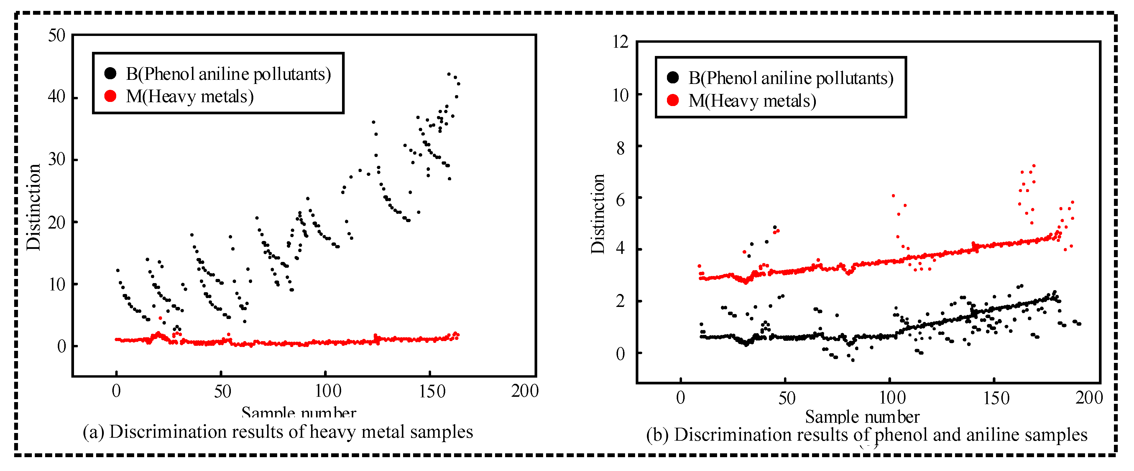
4.3. Recognition and Classification of Polluted Marine Environment by K-Means Clustering Algorithm

All the above experiments are carried out in unpolluted background seawater, and the effectiveness of the proposed algorithm is discussed. The test will be conducted with real datasets, which are derived from Argo buoy profile data of the Indian Ocean from July to September 2019 obtained by the Argo real-time data center of China, and the data are obtained three times a day. In order to control a single variable, 276 observation data in the same grid (−35.614, 62.896) and the same buoy (1900050) were selected for cluster analysis. Figure 8 shows marine water pollution identification based on K-means clustering.
In Figure 8, the green triangle represents the unpolluted water sample, the blue circle represents the heavy metal polluted water sample, and the red square represents the phenol aniline polluted water sample; (a) and (b) are the clustering based on cosine distance and discrimination, respectively. According to the clustering results, the blue circle and the red square are the water samples in the fixed time series, which shows that the K-means algorithm based on cosine distance and discrimination can better identify the pollution events of marine water. In addition, the results in Figure 8 show that there are some fuzzy samples in the clustering classification based on cosine distance and discrimination. Overall, the classification accuracy based on cosine distance is 89.7%, and the classification accuracy based on discrimination is 95.6%. Compared with the experimental results in Table 6, it can be found that under the actual test, the accuracy of the proposed clustering algorithm is reduced, but there is little difference with the experimental results.
Comprehensive experimental results show that the proposed method has better classification accuracy than the traditional method. When the six water quality parameters are classified and analyzed, it is found that temperature has little effect on the classification results of water pollutants, so the water quality parameter temperature is excluded. Under different cosine distances, the overall classification accuracy of this method is still maintained at a high level, reaching 96.3%. Finally, a case study is carried out to further verify the accuracy of the proposed method, which has a good performance in identifying seawater pollutants.

5. Discussion

On the whole, the study is divided into two stages: one is the detection of marine water quality anomaly, and the other is the classification of water quality anomaly characteristics. The two stages of the study involve the use of data mining technology, and the method proposed in this study has certain advantages compared with other existing studies.
Samendra et al. compared the effects of three sensors with different principles on the real-time detection of microorganisms in reclaimed water, and they found that the sensor based on the Adenosine triphosphate (ATP) production principle had the best effect on microbial detection [16]. The research results of Samendra et al. show that different water quality detection targets need to select corresponding sensors. This research is aimed at early warning of marine water body anomalies quickly and effectively. Therefore, the research chooses conventional water quality sensors for real-time detection, and it uses the x-control chart algorithm to cooperate with early warning, which improves the efficiency of water quality early warning. Wang et al. studied the early warning of water quality and proposed an LS-SVM model to quantitatively evaluate the detection effect of water quality. The results verified the generalization ability and accuracy of the model [17]. From their results, the model can better solve the local nonlinear problem of long-term water quality monitoring, but in the short-term anomaly early warning, the accuracy of the model is limited. In this study, anomaly detection is carried out for short-term data, and the misjudgment rate is below 4.17%, which is a supplement to the research of short-term water quality anomaly early warning direction.
The other stage of the study is the classification of water quality anomaly characteristics. Vasilescu et al. established an efficient method for fluorescent water compound recognition, which used artificial neural network processing technology for on-line identification of marine oil spill, and they verified its feasibility [18]. Their research idea is to reveal the distribution of fluorescent water components by using the channel relationship, and the sensitivity of the recognition model depends on the training dataset and training rules. In contrast, the research method in this paper pays more attention to the judgment of the similarity of the research object, that is, the classification accuracy, and it does not consider the classification sensitivity. Based on the idea of machine learning, Xu et al. studied the online early warning technology of water pollution, and they confirmed that the early warning accuracy of the pcc-svm model proposed by Xu is more than 88% [19]. Júnez-Ferreira et al. designed a groundwater monitoring network with spatiotemporal variability by combining geostatistical methods, which visualized the characteristics of water quality anomalies, which is a new idea for water quality anomaly positioning [20]. This study focuses on the identification of water pollution types, and the accuracy of discrimination classification is more than 95.6%, which is conducive to the rapid development of relevant treatment measures when marine water pollution occurs. However, compared with other studies, this study is obviously weak in the positioning of water quality anomalies, which needs to be made up in future studies [21,22].

6. Conclusions

At present, more and more serious sea water pollution has become a research hotspot of scholars all over the world. In order to detect and control the impact of marine water pollution in time, a six-parameter water quality model was proposed to detect and early warn the marine water anomalies. On the other hand, the K-means clustering technology in data mining is used to quickly identify the types of water pollution, and the concept of “discrimination” with higher classification accuracy is proposed. The results show that the detection rates of heavy metal pollutants and phenol aniline pollutants are 94.7% and 97.8%, respectively, and the total classification accuracy of seawater pollutants is 96.3% under the K-means clustering analysis based on discrimination. In addition, the real datasets are tested, and the results show that the classification accuracy based on the cosine distance and discrimination is 89.7% and 95.6%, respectively. In addition, there are some deficiencies in the research results. First, there is a certain correlation between water quality parameters, but this study did not conduct an in-depth discussion on this aspect. Second, the study only analyzed two types of marine pollutants; thus, the breadth of the study is lacking. In the next study, on the one hand, the correlation between water quality parameters and various pollutants will be deeply explored; on the other hand, the types of pollutants involved in the study will be expanded to verify the universality of the research method in practical application. In this paper, the characteristics of marine water pollution are analyzed and judged, but the possible changes of water quality in the future are not reasonably predicted. Therefore, in the future research, more years of historical water quality data analysis should be considered to explore the change trend of water quality and provide a more theoretical basis for marine water protection.

Author Contributions

Conceptualization, H.L. and J.C.; methodology, H.L.; software, J.C. and X.B.; validation, X.B.; formal analysis, H.L.; investigation, X.B.; resources, J.C.; data curation, J.C.; writing—original draft preparation, H.L.; writing—review and editing, X.B.; visualization, X.B.; supervision, J.C.; project administration, H.L.; funding acquisition, X.B. All authors have read and agreed to the published version of the manuscript.

Funding

This research received no external funding.

Institutional Review Board Statement

Not applicable.

Informed Consent Statement

Not applicable.

Data Availability Statement

All data generated or analysed during this study are included in this published article.

Conflicts of Interest

The authors declare no conflict of interest.

References

  1. Subbiah, S.; Karnjanapiboonwong, A.; Maul, J.D.; Wang, D.; Anderson, T.A. Monitoring cyanobacterial toxins in a large reservoir: Relationships with water quality parameters. PeerJ 2019, 7, e7305. [Google Scholar] [CrossRef] [PubMed]
  2. Farnham, D.J.; Gibson, R.A.; Hsueh, D.Y.; McGillis, W.R.; Culligan, P.J.; Zain, N.; Buchanan, R. Citizen science-based water quality monitoring: Constructing a large database to characterize the impacts of combined sewer overflow in New York City. Sci. Total Environ. 2017, 580, 168–177. [Google Scholar] [CrossRef] [PubMed] [Green Version]
  3. Griffith, J.F.; Weisberg, S.B.; Arnold, B.F.; Cao, Y.; Schiff, K.C.; Colford, J.M., Jr. Epidemiologic evaluation of multiple alternate microbial water quality monitoring indicators at three California beaches. Water Res. 2016, 94, 371–381. [Google Scholar] [CrossRef]
  4. Majid, N.; Muhammad, B. Evaluation of Ordinary Least Square (OLS) and Geographically Weighted Regression (GWR) for Water Quality Monitoring: A Case Study for the Estimation of Salinity. J. Ocean Univ. China 2018, 2, 305–310. [Google Scholar]
  5. Pérez, C.J.; Vega-Rodríguez, M.A.; Reder, K.; Flörke, M. A Multi-Objective Artificial Bee Colony-based optimization approach to design water quality monitoring networks in river basins. J. Clean. Prod. 2017, 166, 579–589. [Google Scholar] [CrossRef]
  6. Hamid, A.; Bhat, S.A.; Bhat, S.U.; Jehangir, A. Environmetric techniques in water quality assessment and monitoring: A case study. Environ. Earth Sci. 2016, 75, 321–334. [Google Scholar] [CrossRef]
  7. Delpla, I.; Florea, M.; Rodriguez, M.J. Drinking Water Source Monitoring Using Early Warning Systems Based on Data Mining Techniques. Water Resour. Manag. 2019, 33, 129–140. [Google Scholar] [CrossRef]
  8. Sun, Q.; Zhang, J.; Xu, X. Research and Application of Rule Updating Mining Algorithm for Marine Water Quality Monitoring Data. Pol. Marit. Res. 2018, 25, 136–140. [Google Scholar] [CrossRef] [Green Version]
  9. Cominola, A.; Nguyen, K.; Giuliani, M.; Stewart, R.A.; Maier, H.R.; Castelletti, A. Data Mining to Uncover Heterogeneous Water Use Behaviors from Smart Meter Data. Water Resour. Res. 2019, 55, 9315–9333. [Google Scholar] [CrossRef] [Green Version]
  10. Lee, S.; Hyun, Y.; Lee, M.J. Groundwater Potential Mapping Using Data Mining Models of Big Data Analysis in Goyang-si, South Korea. Sustainability 2019, 11, 1678. [Google Scholar] [CrossRef] [Green Version]
  11. Govender, P.; Sivakumar, V. Application of k-means and hierarchical clustering techniques for analysis of air pollution: A review (1980–2019)—ScienceDirect. Atmos. Pollut. Res. 2020, 11, 40–56. [Google Scholar] [CrossRef]
  12. Mahajan, M.; Kumar, S.; Pant, B. Prediction of Environmental Pollution Using Hybrid PSO-K-Means Approach. Int. J. E-Health Med. Commun. (IJEHMC) 2021, 12, 65–76. [Google Scholar] [CrossRef]
  13. Ahmadmoazzam, M.; Birgani, Y.T.; Molla-Norouzi, M.; Dastoorpour, M. Assessment of the Water Quality of Karun River Catchment Using Artificial Neural Networks-self-Organizing Maps and K-Means Algorithm. J. Environ. Account. Manag. 2020, 9, 43–58. [Google Scholar] [CrossRef]
  14. Li, T.; Sun, G.; Yang, C.; Liang, K.; Ma, S.; Huang, L. Using self-organizing map for coastal water quality classification: Towards a better understanding of patterns and processes. Sci. Total Environ. 2018, 628–629, 1446–1459. [Google Scholar] [CrossRef] [PubMed]
  15. Hu, M.; Jia, L.; Wang, J.; Pan, Y. Spatial and temporal characteristics of particulate matter in Beijing, China using the Empirical Mode Decomposition method. Sci. Total Environ. 2013, 458–460, 70–80. [Google Scholar] [CrossRef]
  16. Samendra, S.; Syreeta, M.; Luisa, I.; Yu, H.W.; Snyder, S.A.; Pepper, I.L. Near Real-Time Detection of E. coli in Reclaimed Water. Sensors 2018, 18, 2303. [Google Scholar] [CrossRef] [Green Version]
  17. Wang, K.; Wen, X.; Hou, D.; Tu, D.; Zhu, N.; Pingjie, H.; Guangxin, Z.; Zhang, H. Application of Least-Squares Support Vector Machines for Quantitative Evaluation of Known Contaminant in Water Distribution System Using Online Water Quality Parameters. Sensors 2018, 18, 938. [Google Scholar] [CrossRef] [Green Version]
  18. Vasilescu, J.; Marmureanu, L.; Carstea, E. Analysis of Seawater Pollution Using Neural Networks. Rom. J. Phys. 2011, 56, 530–539. [Google Scholar]
  19. Xu, X.; Liu, Y.; Liu, S.; Li, J.; Guo, G.; Smith, K. Real-time detection of potable-reclaimed water pipe cross-connection events by conventional water quality sensors using machine learning methods. J. Environ. Manag. 2019, 238, 201–209. [Google Scholar] [CrossRef]
  20. Júnez-Ferreira, H.E.; Herrera, G.S.; Saucedo, E.; Pacheco-Guerrero, A.I. Influence of available data on the geostatistical-based design of optimal spatiotemporal groundwater-level-monitoring networks. Hydrogeol. J. 2019, 27, 1207–1227. [Google Scholar] [CrossRef]
  21. Xie, T.; Liu, R.; Wei, Z. Improvement of the fast clustering algorithm improved by k-means in the big data. Appl. Math. Nonlinear Sci. 2020, 5, 1–10. [Google Scholar] [CrossRef] [Green Version]
  22. Wu, J.; Yuan, J.; Gao, W. Analysis of fractional factor system for data transmission in SDN. Appl. Math. Nonlinear Sci. 2019, 4, 191–196. [Google Scholar] [CrossRef] [Green Version]
Figure 1. Schematic diagram of the basic structure of the X control chart.
Symmetry 13 00355 g001
Figure 2. Schematic diagram of the polygon area method.
Symmetry 13 00355 g002
Figure 3. Schematic diagram of the six-parameter feature map without pollutants.
Symmetry 13 00355 g003
Figure 4. Changes of six water quality parameters over time.
Symmetry 13 00355 g004
Figure 5. Broken line chart of water quality Anomaly Index Y.
Symmetry 13 00355 g005
Figure 6. Clustering effect of water samples with different pollution types based on cosine distance.
Symmetry 13 00355 g006
Figure 7. Clustering effect of water samples with different pollution types based on discrimination.
Symmetry 13 00355 g007
Figure 8. Identification of marine water pollution based on K-means clustering.
Symmetry 13 00355 g008
Table 1. Water quality status judgment table.
Hexagon Area YAbnormal Water Quality Index SWater Quality Status
≤1<23.4Normal
>1<23.4Abnormal
>1≥23.4Severe abnormality
Table 2. Output correlation.
Forecast Water Quality AbnormalitiesCorresponding ParametersForecast of Normal Water QualityCorresponding Parameters
Actual water quality is abnormalTrue positiveTPFalse positiveFP
Actual water quality is normalFalse negativeFNTrue negativeTN
Table 3. Evaluation of abnormal water quality detection results.
PollutantsFPTNFNTPFARPDFCR
Phenolanilines (113)06112900%88.2%7.36%
Heavy metals (119)24651304.17%96.3%3.83%
Table 4. Evaluation of water quality anomaly detection results by other methods.
PollutantsMolecular MethodHyserve Method
FARPDFCRFARPDFCR
Phenolanilines (113)10%91.30%8.63%7%84.30%7.36%
Heavy metals (119)12.40%85.50%7.64%9.23%74.26%5.97%
Table 5. Experimental groups and parameters.
GroupIncluded ParametersClassification Accuracy (%)
Group AK, pH, ORP, DO, UV254, T90.52
Group BK, pH, ORP, DO, UV25492.36
Group CT, pH, ORP, DO, UV25489.74
Group DK, T, ORP, DO, UV25486.13
Group EK, T, pH, ORP, UV25482.37
Group FK, T, pH, DO, UV25481.63
Group GK, T, pH, ORP, DO80.99
Table 6. Comparison of classification accuracy and cosine distance of pollutants.
ClassificationClassification Accuracy of Heavy Metal SamplesCorrect Rate of Classification of Phenol Aniline SamplesOverall Classification
Accuracy
Discrimination94.7%97.8%96.3%
Cosine distance94.9%91.5%93.2%
Publisher’s Note: MDPI stays neutral with regard to jurisdictional claims in published maps and institutional affiliations.

