Article

Comparative Analysis of the Life-Cycle Cost of Robot Substitution: A Case of Automobile Welding Production in China

School of Management, Hefei University of Technology, No. 193 Tunxi Road, Hefei 230000, China
*
Author to whom correspondence should be addressed.
Symmetry 2021, 13(2), 226; https://doi.org/10.3390/sym13020226
Submission received: 1 December 2020 / Revised: 25 January 2021 / Accepted: 27 January 2021 / Published: 29 January 2021

Abstract

:
Within the context of the large-scale application of industrial robots, methods of analyzing the life-cycle cost (LCC) of industrial robot production have shown considerable developments, but there remains a lack of methods that allow for the examination of robot substitution. Taking inspiration from the symmetry philosophy in manufacturing systems engineering, this article further establishes a comparative LCC analysis model to compare the LCC of the industrial robot production with traditional production at the same time. This model introduces intangible costs (covering idle loss, efficiency loss and defect loss) to supplement the actual costs and comprehensively uses various methods for cost allocation and variable estimation to conduct total cost and the cost efficiency analysis, together with hierarchical decomposition and dynamic comparison. To demonstrate the model, an investigation of a Chinese automobile manufacturer is provided to compare the LCC of welding robot production with that of manual welding production; methods of case analysis and simulation are combined, and a thorough comparison is done with related existing works to show the validity of this framework. In accordance with this study, a simple template is developed to support the decision-making analysis of the application and cost management of industrial robots. In addition, the case analysis and simulations can provide references for enterprises in emerging markets in relation to robot substitution.

1. Introduction

Since the 1970s, the industrial robot has been widely used in industrialized countries in manufacturing processes, subsequently becoming the core of modern manufacturing [1]. Since 2012, the global industrial robot holding volume has grown at an average annual rate of 15.2%. Although the large-scale application of industrial robots in the manufacturing sector started late in China, it has sustained an average annual growth rate of 28%, much higher than that of other countries [2]. This trend is expected to be maintained in the next decade due to the rising labor cost, the upgrading of industrial structure, and the fierce global competition [3]. However, in the context of the “robot substitution”, numerous problems have emerged in Chinese enterprises such as the challenge of running industrial robots with other production systems, the difficulty of cultivating robot professionals, and the high expenditure after robot introduction. In some cases, compared with traditional production, it seems that the industrial robot is unaffordable [4]. In fact, most enterprises focus on the initial investment, but the huge life-cycle costs (LCC) are ignored. In addition, due to the lack of a corresponding analysis approach, it is difficult to clearly estimate the cost of “robot substitution”, resulting in decision-making risks and unmanageable costs [5]. To determine whether industrial robot substitution is economically viable, it is necessary to establish a comparative analysis framework of LCCs and compare the cost and cost-efficiency of the two manufacturing modes during the lifespan. Thus, the following questions were identified: What costs do the LCCs of the two manufacturing modes include? How do the LCC components change at different stages? How can the dynamic cost (the tendency of the total cost structure) of the two manufacturing modes over their life cycle be scientifically analyzed? Does industrial robot production have a cost advantage over traditional production in the life cycle? How does it perform over its lifespan in terms of total cost, unit cost, and cost structure? What factors mainly affect and restrict this cost advantage (if there are any)? Finally, what can we learn from it?
LCC is a well-known cost analysis method, first applied in the UK in the late 1950s, that considers all related expenses in support of one item, from its initial development to the final scrapping [6]. Traditionally, it is considered mostly as a support tool in investment in fixed assets, such as property, machinery, plant, and infrastructure. However, from a wider perspective, LCC is now viewed as a strategic tool for the lifecycle management of manufacturing assets [7], and it plays a larger role in decisions supporting asset procurement [8], asset configuration [9], and asset operations [5], contributing to the product–service system [10]. Scholars have developed various methods and discussed the LCCs of manufacturing systems, and the LCC of industrial robots is now becoming a hot topic in current research [11]. Some studies have discussed heterogeneous cost factors of industrial robots over their life cycle [12,13] and preliminarily established the cost structure of the LCC [5]. On this basis, a few LCC analyses are conducted with the help of simulation technology [12,13] and case studies [5,14]. In regard to “robot substitution”, it can be found that some economic models have been developed to conduct a quantitative comparison of cost efficiency between industrial robot and traditional manual manufacturing systems [15,16,17]. Nevertheless, current research still lacks LCC comparison between industrial robot production and traditional manual production, representing a research gap.
It is widely considered that space–time symmetry is ubiquitous in the universe, and there are lots of symmetric problems waiting to be discovered and studied in every field [18]. To contribute to filling the gap above, taking inspiration from the symmetry philosophy in manufacturing systems engineering, this study further examines the LCC of robot substitution and presents a comparative analysis of the LCC of robot substitution. At first, it establishes a comparative LCC model, integrating industrial robot production and traditional production into the framework. Then, it conducts a case analysis and simulations from a Chinese automobile manufacturer and compares the LCC of welding robot production with manual welding production. In this study, intangible costs are introduced (covering idle loss, efficiency loss, and defect loss) to supplement the actual costs, constituting a relatively complete cost breakdown structure. Meanwhile, various methods are comprehensively used for cost allocation and variable estimation in order to conduct total cost and the cost efficiency analysis, together with hierarchical decomposition and dynamic comparison. It involves the symmetry and asymmetry of the following: industrial robot production and traditional production in terms of “robot substitution”, the actual and intangible costs, the LCC structure, and the manufacturing system and external environment.
This study makes the following contributions. (i) Previous studies mainly focus on LCC analysis of industrial robots, paying more attention to the total ownership cost over the life cycle [5,12], while the current study is the first study that conducts comparative LCC analysis of robot substitution, providing a comparative analysis framework of dynamic costs for the two manufacturing modes. (ii) Existing LCC models of industrial robots mostly highlight the actual costs. Although the cost factors related to intangible loss in production have received extensive attention, intangible costs have not been clearly defined and measured [5,13]. This study integrates the actual and intangible cost (covering idle loss, efficiency loss, and defect loss) to form a complete LCC structure, which helps to clearly reflect the dynamic cost-efficiency of robot substitution. (iii) Considering the availability and integrity of the database, most of the existing literature uses simulation technology to estimate the LCC of industrial robots [11], and empirical analysis of the cost efficiency of robotic implementation is relatively scarce [14]. Combined with case analysis and simulation, this study performs a comparative cost–benefit analysis of robot substitution with the help of operation records over the life cycle, and it obtains some valuable results. (iv) Most of the relevant research comes from industrial countries, and there is little literature regarding emerging markets [5]. This paper conducts a case analysis and simulations of a Chinese manufacturer, which enriches the relevant literature. The structure of this paper is arranged as follows. After the introduction, this paper provides a theoretical background. Then, the materials and methods are discussed. Afterwards, a case analysis and simulations are conducted. The results are then presented and discussed, and the conclusion is obtained from the perspective of management.

2. Theoretical Background

2.1. Cost Breakdown Structure of LCC

LCC mainly focuses on the process of obtaining and applying fixed assets [10], which requires a full consideration of the costs associated with the acquisition, ownership, usage, and subsequent disposal [19]. All of the disbursement during the life span, including the demand assessment, concept, design, manufacturing, operation, disposal costs, etc. [8], can be divided into four categories, namely research and development cost, production and consumption cost, operating and maintenance cost, and retirement and disposal cost [20]. Its specific breakdown depends on the cost characteristic, the information heterogeneity, and the available data [21]. Previous studies show that in LCC structure, the utilization cost is much higher than the acquisition cost and a longer life cycle corresponds to a lower unit total cost, as well as a higher average return [22]. Traditional LCC models focus on the actual cost and ignore the intangible cost [8]. However, when comparing the cost among projects, the productivity loss should not be neglected [23]. It is recognized that when the asset fails, the potential output gains lost should be quantified since the asset is out of service [24,25]. Moreover, additional resources are utilized to maintain a smooth manufacturing process in order to ensure operational reliability [26]. In addition, substandard product quality or reduced productivity may cause a huge amount of waste [25]. Furthermore, some business uncertainties and decision risks can lead to production disruption, leaving equipment and workers waiting [27]. Based on the literature above, the potential productivity loss, or “gains from cost savings”, should be considered separately and clearly classified as intangible cost [23]. Hence, we can obtain a clear outline of the cost breakdown structure, which divides the total cost into actual cost and intangible cost. The actual cost can be subdivided into several components according to the characteristics of the LCC structure, and the intangible cost mainly refers to the potential cost caused by idle loss, efficiency loss, quality loss, etc. [15,16,28].
Many studies have discussed the cost breakdown structure of the automatic manufacturing systems related to industrial robots. One representative study builds the LCC framework of heavy machinery systems, divides the total cost into ownership and operation costs, subdivides the operation costs into explicit and stealth operation costs, and categorizes the related cost factors [29]. Another study examines the LCC of computer information systems; decomposes the total cost into initial, operation, and disposal costs; and analyzes their drivers [30]. Another study establishes an LCC framework of industrial robots; divides the total cost into acquisition, operation, and disposal costs; summarizes various cost drivers; and examines the quality cost factors [5]. Some scholars investigate the LCC of robot systems; argue that the costs in the debugging, upgrading, maintenance, and disposal processes can be easily ignored; and examine the related cost factors in depth [12,13]. Some scholars have examined the LCC of electronic equipment components [31] and examined in depth the disposal costs, including the costs associated with depreciation and the expenses related to disposal, while others have investigated the LCC of cloud computing services, with emphasis on the relevant costs of equipment procurement [32]. In addition, intangible costs are thoroughly examined in some LCC models, and their cost factors are discussed [9,14,29]. Given the similarities in the cost structures, most of these frameworks have defined and subdivided acquisition, operation, maintenance, and disposal costs, as well as intangible costs, forming a relatively clear framework. However, compared with the actual cost, the intangible cost has not been clearly defined [8]. Overall, there is still a lack of an integrated framework between actual and intangible costs, making comparative analysis difficult.

2.2. Cost Factors Related to the LCC of Robot Substitution

Industrial robot production refers to the manufacturing mode of using highly integrated automation equipment, while traditional production is the manufacturing mode that mainly relies on manual operation machine [33]. Scholars emphasize that the industrial robot, as a special piece of equipment, has a high total ownership cost and investment risk over its life cycle. They argue that some related costs can be easily ignored and examine the cost factors of LCC in-depth [12]. The LCC of industrial robot production needs to be adequately evaluated with respect to the life cycle production task, which is characterized by the product properties, manufacturing process, technologies steps, output scale, and lot-sizes, as well as the corresponding resource consumption [11]. During investment, the industrial robot is designed according to manufacturers’ needs, and components are purchased or developed and then integrated. This life-cycle phase continues from negotiation to acceptance tests, and the typical cost-relevant expenditure should be treated as investments and allocated over the life cycle [13]. At the beginning of the operation phase, a transient decrease in the output or increase in scrap might result from the running-in process, which induces additional direct cost and opportunity costs. Moreover, another important cost factor is the training of the operators. After the running-in process, the benefits of the industrial robot materialize, as the increasing output, quality, or productivity causes cost savings [34]. Maintenance is considered as a relatively independent life-cycle phase, since it interrupts the operation of the industrial robot. Cost considerations for regular inspections, repair work, and reconfiguration are significantly different from those of operation, since the related expenditures regard the guarantee of sustainable production over the life cycle [12,35]. At the end of the life cycle, the industrial robot will be decommissioned for the following reasons, among others: the operation and maintenance costs continue to rise, it does not fulfil the quality standards, and it is not feasible for new products when a new robot with better cost–benefit ratio is available. Consequently, the disposal expenditure and the residual value should be considered [14].
For traditional production, labor is the most critical factor. Drawn on the LCC structure of equipment, the costs for labor are suggested to be divided into three basic categories: employment costs, which indicate administrative costs related to employees; operating costs, which are those associated with employee compensation; and work environmental costs, which refer to the expenses related to the security and welfare of employees [36]. It is generally believed that administrative costs included in production costs could be further divided into three sub-categories, namely, recruitment costs, education costs, and additional costs (other management fees spent on workers) [37]. Moreover, employee compensation, including salary, performance, overtime pay, subsidies, etc., should be regarded as the direct production cost [38]. Furthermore, the welfare costs, which are the expenses spent on employees, such as social security, medical insurance, retirement, vacation, sick leave, paid vacation, and housing, should be included in indirect production costs [39]. In addition, considering the low value of manual operation equipment, all production costs other than labor costs and administrative costs can be lumped into operation cost, covering direct materials, and related overheads. Examples include materials, power, depreciation on buildings and equipment, maintenance, and so on [40,41,42].
From the literature, we summarize the LCC-related cost factors of two manufacturing modes, and further clarify the key factors that need to be paid attention to in the LCC framework of robot substitution, allowing for the preparation of model construction.

2.3. Cost Measurement and Estimation Methods

In the field of engineering economics, the NPV (net present value) method is widely used to analyze the costs and benefits of projects [43]. It emphasizes the time value of money, which reflects future inflation and interest rates, while the present value represents the value that should be reserved today for future expenditures. In this approach, the expenditure at different times over the life span can be converted into the present value using an appropriate discount rate.
There are three representative methods for estimating costs, namely estimating by engineering procedures, estimating by analogy, and parametric estimation, which apply to heterogeneous costs [44]. The actual costs are suitable for the methods of estimating by engineering procedures, such as the process cost method and the operation cost method. The former focuses on the impact of processes on the overall cost, which is reasonably distributed to each link [45], and the latter emphasizes the “cost driver” in the course of operation and accurately accumulates and allocates the resources consumed in the production process [46]. According to ISO, the accelerated depreciation method can be used for high-tech equipment, while the composite life or annual output proportion method for cost allocation is adopted for general electromechanical. The expenditures for technician training, which is considered the investment in human capital, can be depreciated with high-tech equipment, while technician compensation, energy consumption, consumables, and other expenses are regarded as the current production cost. In addition, the impairment and disposal expenses incurred during the scrapping of assets are apportioned based on the proportion of each annual output [47].
Furthermore, the intangible cost is suitable for the methods of analogy and parametric estimation. One of the most well-known tools is overall equipment efficiency (OEE), which mainly focuses on the factors of availability, performance, and quality [48]. Moreover, the value system cost method facilitates estimation of the value-added loss [49], while the activity-based costing method establishes the activity-based cost standard and can measure the opportunity loss based on time [50]. All of these parameters can be improved to estimate intangible costs from equipment idleness, work inefficiency, and substandard quality [14]. The parameter, presenting a prediction of possibility or cost rate over the life cycle, is mainly estimated based on probabilistic/stochastic methods. Most studies related to industrial robots apply computer simulation technology to estimate the relative parameters [12,13,15]. However, considering the complexity of the manufacturing system, its accuracy needs to be improved [16]. In contrast, it might be more convenient and reliable to conduct estimations with the help of statistical analysis from operation records, although this method is limited by the availability of appropriate data [51]. Drawing on the discussion, we must first convert all the expenditures over the life span into NPV at first. As for actual costs, we should collect and allocate them using appropriate methods according to the nature of each item. Finally, regarding intangible costs, we can set reasonable parameters to estimate them with the help of operational records of the life cycle.

3. Materials and Methods

Given the complexity in conducting the comparative analysis of LCC of robot substitution, first, the theoretical framework is established and the cost drivers are clarified. Second, the LCC model of robot substitution is constructed in accordance with the cost breakdown structure. We define the formulas to calculate total cost, cost efficiency, and substitution coefficient of the two manufacturing modes that could clearly reflect the cost composition, comparative advantage, and dynamic cost. Third, the measurement and estimation methods of various costs are identified. Due to the significant differences in costing, we adopt multiple approaches for heterogeneous costs. Finally, the method of case analysis and simulation is briefly introduced.

3.1. Comparative LCC Model of Robot Substitution

Combining literature collection with field investigation, we sort out heterogeneous costs incurred during the life cycle of the two manufacturing modes respectively and summarized them into one comparative LCC structure, which can reflect the cost characteristics of production procedure at the same time. The comparative LCC structure and cost drivers are as shown in Table 1. The LCC structure of industrial robot production is defined as investment, operation, maintenance, disposal, and intangible costs; and that of the traditional production is defined as management, compensation, welfare, operation, and intangible costs. Where C R is the total cost of the industrial robot production in terms of actual costs; C R I refers to investment cost, including items such as equipment price, transaction cost, loan interest, taxes minus subsidies, after-sales fee, etc. [5,9,12,13,14]; C R O refers to operation cost, including items such as operator’s remuneration, training expenditure, spend on pace, accessories charge, energy consumption, etc. [5,9,12,13,14]; C R M refers to maintenance cost, including items such as service fee, replacing parts price, consumables charge, annual inspection fee, etc. [5,9,12,14]; C R D refers to disposal cost, including demolition expenses minus residual value, etc. [5,9,14]; C T is the total cost of the traditional production in terms of actual costs; C T M refers to management cost, including recruitment expenditure, training expenditure, labor protection expense, office expense etc. [36,37,38,39,40,41,42]; C T C refers to compensation cost, including basic salary, performance bonus, overtime pay, work subsidy, etc. [36,37,38,39]; C T W refers to welfare cost, including social security charges, housing fund, trade union funds, daily welfare expenses, etc. [36,37,38,39]; C T O refers to operation cost, including equipment depreciation, equipment maintenance, material consumption, energy consumption, spend on pace, tool amortization, etc. [40,41,42]. In addition, C O R and C O T represent the intangible costs of the two production modes, respectively, covering production idle loss, product efficiency loss, product defect loss, etc. [15,16,17]. The total cost of robot production is shown in Equation (1), and the total cost of traditional production is shown in Equation (2).
C R = C A   R + C O   R = C R I + C R O + C   R M + C   R D + C O   R
C T = C A   T + C O   T = C T M + C T C + C   T W + C   T O + C O   T
Cost efficiency reflects the productivity of cost expenditure. It is calculated as a ratio of the total cost, as well as its components to the output during the current period. The actual total cost is decomposed into components according to Equation (1) and then divided by the output quantity so the unit cost of each component is obtained. This is shown in Equations (3) and (4), where Q R is the output of the industrial robot production, A C R is C R per unit output of the industrial robot production, similar to A C R I , A C R O , A C R M , A C R D , and A C O R ; Q T is the output of the traditional production, A C T is C T per unit output of the traditional production, similar to A C T M , A C T C , A C T W , A C T O , and A C O T .
A C R = C R / Q R * 100 = A C R I + A C R O + A C   R M + A C   R D + A C O   R
A C T = C T / Q T * 100 = A C T M + A C T C + A C   T W + A C   T O + A C O   T
The substitution coefficient reflects the comparative advantage of LCC and is calculated as the ratio of the cost efficiency of the two manufacturing modes. This is shown in Equation (5), where S C R T refers to the substitution coefficient of the two manufacturing modes. When S C R T > 1 , industrial robot production has a comparative advantage over traditional production; when S C R T = 1 , the cost efficiency of the two is equal; when S C R T < 1 , traditional production is considered the more economical method.
S C R T = A C T / A C R

3.2. Cost Allocation and Variables Estimation

Taking into account the time value of money, all expenditures involved during the life span should be converted to N P V before being carried forward to the actual cost. This is shown in Equation (6), where N P V refers to the net present value, P V refers to the actual expenditure, R refers to the discount rate (benchmark interest rate), and n refers to the rank in the lifecycle.
N P V = P V / ( 1 + R ) n
In the actual cost measurement, in order to accurately reflect the dynamic cost, it is necessary to allocate the capitalized expenditure reasonably to each year. As high-tech production equipment, industrial robots are suitable for the accelerated depreciation method, and C R I adopts the sum of years digits method for cost allocation. C R O is regarded as the current cost, while C R M and C R D are apportioned based on the output. The traditional production follows a conservative method, in which the value of equipment is firstly depreciated according to the output and then C T M , C T C , C T W , and C T O are directly accounted for in the current cost. Furthermore, the intangible cost is usually estimated with the help of relevant parameters. Based on the literature discussed above, the estimation methods of C O R and C O T are developed, as shown in Equations (7)–(11), where T I is the idle production time, T M is the maintenance time, T S is the saturated working time, r I is the idle loss rate, r E is the efficiency loss rate, r U is the unqualified product rate, r V is the added value rate, A P is the value of the finished product, and A C A is the actual cost per unit output.
r I = T I / T S
r E = T M   / T S
r V = ( A P A C A ) / A C A
C O R   = ( C R I + C R O + C   R M + C   R D ) * r V * ( r I + r E + r U )
C O   T = ( C T M + C T C + C   T W + C   T O ) * r V * ( r I + r E + r U )

3.3. Data Resources

Industrial robots are widely used in the automotive manufacturing industry, and the welding robot is the most commonly used. Hence, a Chinese automobile enterprise is selected as a sample, and the application of welding robots in the production is investigated. In this case, all the products are initially welded by hand-operated welding machines. In 2006, the welding production line introduced 15 sets of Hyundai hx165 electric welding robots. After that, the welding operation was divided into two parts: industrial robot welding and manual welding. The welding robots are responsible for the welding operation of 2454 welding points outside the body-in-white, while the manual welding is responsible for 1418 welding points inside it. The two manufacturing modes are fairly similar in terms of their product attributes and quality requirements. By the end of 2019, these robots were scrapped. The main machining cells of the two manufacturing modes are shown in Figure 1.
In this case, industrial robots are introduced by financial leasing at a price of CNY 600,000 per unit and settled in the form of mortgage payments. The designed life cycle of the industrial robot is 15 years. The actual life span of the welding industrial robots was from 2006 to 2019, lasting 14 years. Five engineers are trained to be in charge of operating the welding robot. Moreover, regular maintenance is carried out every year, while special maintenance is carried out according to the production arrangements. Industrial robots were scrapped one year ahead of schedule with a small residual value and high dismantling costs. At the same time, the manual welding production process was divided into 5 production teams with a total of 50 employees. Twenty spot welders are used in the traditional production with a value of CNY 27,000 per unit. The actual life cycle of these tools is synchronized with industrial robots, and this whole value is allocated to operating costs without residual value. The data involved in the actual cost originate from accounting data and the data involved in intangible cost come from historical production records. All the data are verified by material collection and on-site interviews.

3.4. Case Analysis and Simulation

The case analysis was firstly conducted, in which a comparative cost–benefit analysis of robot substitution with the help of operation records over the life cycle was performed. Then, simulations were carried out in order to overcome the shortcomings of the case analysis and extend the model to more scenarios. Based on the comparative LCC model of industrial substitution, an LCC system dynamics model was built in Vensim software, and parameters were set with reference to the empirical data from the case analysis. Then, the LCCs of welding robot production and manual welding production were modeled and simulated, respectively. The simulation mainly focused on four heterogeneous factors affecting the LCC of robot substitution, including the fluctuation of production scale, the rise of labor costs, and the number of robots input in industrial robot production and front-line workers input in traditional production. Each of these four factors was divided into two conditions, and every condition is further defined and explained in Table 2. Applying these heterogeneous conditions to the simulation, we can obtain the LCCs of industrial robot production in 8 scenarios, the LCCs of traditional production in 8 scenarios, and the comparative LCCs of industrial robot substitution in 16 scenarios.

4. Results

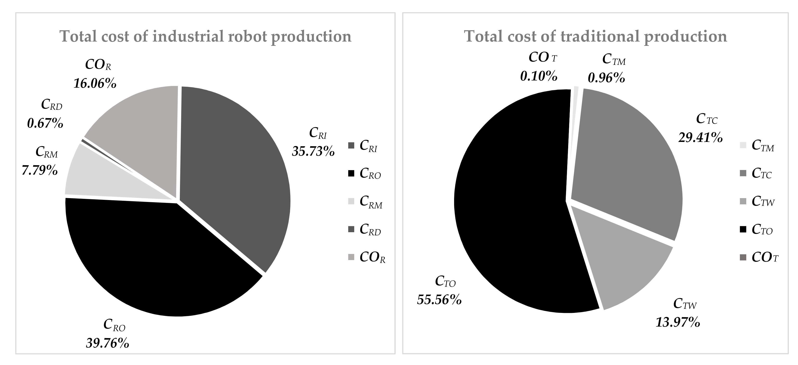
4.1. Comparison of the Total Cost

In case analysis, the total cost and cost efficiency over the life cycle of the two manufacturing modes are computed separately, as shown in Table 3, from which several important findings can be observed. Figure 2 presents the total costs for the two manufacturing modes of the case analysis, and Figure 3 presents that of the simulations.
As shown in Figure 2, C R has two main components, namely, C R I and C R O , which account for 35.73% and 39.76% respectively, making them highly relevant to industrial robotic equipment. The simulation results are the same in most scenarios, as shown in Figure 3. This is also in line with the findings of Landscheidt [14], Dietz et al. [12], and Zwicker et al. [13]. Meanwhile, C T O , C T C and C T W account for relatively high proportions in the traditional production of 55.56%, 29.41%, and 13.97% respectively, suggesting that they are deeply affected by labor costs. The simulation results are the same in most scenarios, as is shown in Figure 3. This is similar to the prior studies of Adegbola etc. [38] and Barosz etc. [16]. This indicates that industrial robot production is typically characterized by a huge initial investment on manufacturing assets, while traditional production highly relies on skilled labor force. So the industrial robot creates high fixed costs and low variable costs compared to manual work.
Overall, two manufacturing modes show heterogeneous characteristics of the total cost structure. Robot production is typically characterized by a huge initial investment in manufacturing assets, while traditional production highly relies on a skilled labor force [16]. Thus, the industrial robot creates high fixed costs and low variable costs compared to manual work. In addition, industrial robot production has a large proportion of intangible costs, which indicates that the relatively low flexibility leads to significant potential loss [11].

4.2. Comparison of Total Cost Efficiency

Figure 4 presents the comparison of total cost efficiency of the two manufacturing modes of the case analysis, and Figure 5 presents that of the simulations. The case analysis obtained that, A C R is 2.49 cents/piece, which is far lower than A C T (7.72 cents/piece), highlighting the significant competitiveness of industrial robot production in terms of cost efficiency. The simulation results are the same in most scenarios, as is shown in Figure 5. This is also consistent with the findings of Adegbola et al. [38].
As shown in Figure 4, from its internal structure, it can be found that for labor-related costs in traditional production, A C T C is 2.27 cents/piece and A C T W is 1.08 cents/piece, much higher than A C R I (0.89 cents/piece), which represents the share of investment cost of industrial robots for each product. This shows that the investment in industrial robots is diluted over the life cycle and has a strong cost advantage over labor force input. And the simulation results are the same in most scenarios, as is shown in Figure 5.
Moreover, in terms of the costs supporting the operational process, A C T O is 4.29 cents/piece and A C T M 0.07 cents/piece, much higher than A C R O (0.99 cents/piece) and A C R M (0.2 cents/piece). This indicates that the use cost of industrial robots in the whole life cycle is significantly lower than the consumption of traditional production. Moreover, the simulation results are the same in most scenarios, as is shown in Figure 5. This is similar to the prior studies of Adegbola etc. [39]. Moreover, considering the intangible costs, A C O R is 0.39 cents/piece, is much higher than A C O T (0.02 cents/piece). Thus, the impact of intangible loss on the cost efficiency of industrial robot production cannot be ignored, while the impact on traditional production is weak. The simulation results are the same in most scenarios, as is shown in Figure 5. Nevertheless, the intangible costs of industrial robot production seem acceptable due to its robust actual cost advantages [11].

4.3. Comparison of Intangible Cost Factors

From the perspective of the total cost factors in the case analysis, as shown in Table 3, r V of the industrial robot is 37.2%, 13 times larger than that of the manual operation, showing the great productivity of industrial robots. In terms of invisible losses, r I of the industrial robot is 0.472, much higher than that of the manual operation, which indicates that industrial robots have a huge idle cost risk when compared with traditional production. This is inconsistent with the findings of Glaser [52], which indicates that the utilization of industrial robots reached up to 90% and, for manual machines, it was only about 40%–60%. This difference may stem from the heterogeneous manufacturing scenario, including the difficulty of manual handling, automation levels, etc. [16]. Moreover, r E of the industrial robot production is 0.041, which is much higher than that of the traditional production, presenting a larger potential efficiency loss. This is consistent with the findings of Barosz etc. [16], which show that the ratio of failure time to scheduled time of manual production is smaller than that of industrial robot production; that is, it has better availability. On the contrary, Kampa et al. find that the availability of industrial robot production is 0.938, higher than that of traditional production (0.893), and this instability may be due to the higher risk of system failure in industrial robot production [28]. In addition, r U of the traditional production is eight times that of industrial robot production, which reflects huge potential quality loss. This is consistent with extensive research [15,16,17,28]. It is generally believed that due to the higher standard deviation in the Six Sigma method resulting from the inhomogeneous manual labor (e.g., different employee qualifications, worst quality in the night shift), the quality level of traditional production is typically lower than that of industrial robot production.
Figure 6 presents the comparison of intangible cost factors of the two manufacturing modes in the case analysis, and Figure 7 presents that of the simulations. In the simulation system, we set r V with reference to the actual value. The output scale is predetermined, which determines r I . Meanwhile, we simply set r E and r U as logarithmic functions of the output, using empirical data for fitting, and then obtained their values under heterogeneous scenarios. On this basis, we obtained the intangible cost rates. Hence, due to the difference in production scale, intangible cost factors in the simulation present two typical types. Two scenarios,I1III1IV1 andI2III1IV1, were studied as representatives respectively, as shown in Figure 7.
As shown in Figure 6a, initially, both manufacturing modes have a large idle rate due to their low output. Among them, r I of industrial robots is as high as 84.15%, causing huge idle loss. As production expands, r I drops rapidly in both cases. When the output reaches 46,000 vehicles, traditional production reaches saturation and continues to the end of the lifespan. However, when the output reaches the peak of 66,000 vehicles, r I of the industrial robots is at its lowest value of 26.37% and still results in considerable productivity loss. This is similar to the simulations under conditions with a uniform and stable production scale, as shown in the Figure 7e; however, it is significantly different from those under conditions with a sustained rising production scale, as shown in the Figure 7a. As shown in Figure 6b, r E of the two manufacturing modes rises with the output expansion over the life cycle. The r E of traditional production rises from the initial value of 1.60% to its maximum value of 4.10%, while r E of industrial robots increases from 3.52% to 4.55%, indicating that industrial robots have better operation stability under large-scale production. However, compared with traditional production, more time and resources must be invested to maintain smooth operation, resulting in large efficiency losses. This is similar to the simulations under conditions with a uniform and stable production scale, as shown in the Figure 7g; however, it is significantly different from those under conditions with a sustained rising production scale, as shown in the Figure 7c. As shown in Figure 6c, r U of industrial robots is always at a stable and low level over its life cycle, from 0.11% to 0.20%, decreasing in the initial period and rising continuously in the later period. Nevertheless, there is an obvious adaptation process for traditional production: r U decreases in the early stage and remains stable at the level of 0.71–0.75 in the later stage. Despite this, it can be observed that industrial robots have undisputed advantages in product quality. This is similar to the simulations under conditions with a uniform and stable production scale, as shown in the Figure 7f; however, it is significantly different from those under conditions with a sustained rising production scale, as shown in the Figure 7b. Considering rV, rI, rE, and rU comprehensively, as shown in Figure 6d, industrial robots always have a considerably high intangible cost rate, and as output expands, this ratio continues to fall from 32.6% to 12.04%. In contrast, the intangible cost rate of traditional production is small. This is similar to the simulations under condition with a uniform and stable production scale, as shown in the Figure 7h; however, it is significantly different from those under conditions with a sustained rising production scale, as shown in Figure 7d. From the comparison between the two conditions, the idle loss resulting from insufficient output is the main source of the intangible cost of industrial robots, and the high value-added rate further amplifies it. Therefore, as a manufacturing asset with huge initial investment and high productivity, the application of industrial robots has a great potential loss risk.

4.4. Comparison of the Dynamic Cost Efficiency

Figure 8 presents the dynamic cost efficiency of industrial robot production of the case analysis, and Figure 9 presents that of the simulations. As shown in Figure 8, A C R declines, but then rebounds at the end, peaking at 8.13 cents /piece at the beginning, reaching its lowest level of 1.85 cents /piece in 2015, and increasing to 2.18 cents /piece at the end. It can be found that in the early stage, the rapid decline in A C R I and A C O R is a major influencing factor.On the one hand, it is observed that with production expansion, the investment cost is rapidly diluted, and its allocation to the unit output becomes smaller; on the other hand, the potential capacity of industrial robots is brought into actual costs, and idle loss is continuously reduced, which leads to a significant reduction in the unit cost and improved cost efficiency. In the later periods, although A C R I continues to decrease, and A C O R is at a low level, A C R O and A C R M increase rapidly, promoting the growth of A C R .This reflects that, at the later life cycle, with the wear and aging of industrial robots, the costs supporting the operation become increasingly prominent, which increases the unit cost and reduces the cost-efficiency.
As shown in Figure 9, the curve shape of the simulations of dynamic cost efficiency of industrial robot production presents two evolutionary trends on the whole, with significant differences betweenI1 andI2 situations. This indicates that the cost-efficiency of industrial robots is most significantly affected by the change in production scale. Figure 9a–d show that in the four scenarios under conditionI1, the shape of the dynamic cost efficiency curve is similar to that of the case analysis, reflecting the characteristics of rapid expansion of production. Nevertheless, Figure 9e–h present a smoother dynamic cost efficiency curve, which reflects the characteristics of uniform and stable production, quite different from the case analysis. In these scenarios, industrial robot production is able to reach its optimal state more quickly and better exploit its cost-efficiency advantages, maintaining a lower cost per unit product throughout the life cycle. Moreover, other things being equal, the simulations under conditions II1 and II2 are compared. It can be seen from the comparison between Figure 9a,b, Figure 9c,d, Figure 9e,f, and Figure 9g,h that there is little difference in dynamic cost efficiency between the two conditions over the life cycle. This indicates that the rise in labor costs has little impact on the cost efficiency of industrial robot production. Furthermore, with other things being equal, the simulations under conditions III1 and III2 are compared. It can be seen from the comparison between Figure 9a,c, Figure 9b,d, Figure 9e,g, and Figure 9f,h that the unit output cost under condition III2 is significantly higher than that under condition III1, which indicates that the cost efficiency is higher when there is a small number of industrial robots input. As in the unsaturated production scale, large-scale industrial robot investment means more depreciation costs and idle costs
Figure 10 presents the dynamic cost efficiency of traditional production in the case analysis, and Figure 11 presents that of the simulations. As shown in Figure 10, A C T demonstrates an obvious U-shaped curve, which continuously declines from 2006 to 2010 and rebounds from 2011 with a rapid growth rate. The main drivers of this trend include A C T O , A C T C , and A C T W , with A C T O accounting for the largest proportion. These variable costs demonstrate a running-in process at the beginning; and a decrease with the learning curve at an average rate of 8.7% from 2006 to 2010. However, the A C T O starts to grow from 2011 with an average annual growth rate of 9.2%, due to the increase in raw material prices, equipment aging, increasing loss rates, job burnout, etc. Meanwhile, A C T C and A C T W continue to increase at an average annual rate of 12.3%, which indicates that the rapid rise in labor costs can be identified as important factors that promote the growth of A C T .
As shown in Figure 11, the curve shape of the simulations of dynamic cost efficiency of traditional production presents two evolutionary trends on the whole, with significant differences between II1 and II2 situations. This indicates that the cost efficiency of traditional production is most significantly affected by the rise in labor costs. Figure 11b,d,f,h show that in the four scenarios under condition II2, the shape of the dynamic cost efficiency curve is similar to that of the case analysis, reflecting the characteristics of the rapid rise in labor costs. Nevertheless, Figure 11a,c,e,g present a smoother dynamic cost efficiency curve, which reflects the characteristics of relatively stationary labor costs, quite differently from the case analysis. In these scenarios, traditional production can maintain a lower unit cost throughout the life cycle since its main components are labor costs and operation costs, and the latter are relatively stable. Moreover, with other things being equal, the simulations under conditions I1 andI2 are compared. It can be seen from the comparison between Figure 11a,e, Figure 11b,f, Figure 11c,g, and Figure 11d,h that there is little difference in dynamic cost efficiency between the two conditions over the life cycle. This indicates that the fluctuation of production scale has little impact on the cost efficiency of traditional production. Furthermore, with other things being equal, the simulations under conditions IV1 and IV2 are compared. It can be seen from the comparison between Figure 11a,c, Figure 11b,d, Figure 11e,g, and Figure 11f,h that the unit output cost under condition IV2 is significantly higher than that under condition IV1, which indicates that the cost efficiency is higher when there is a small number of front-line workers input. Since labor costs constitute the core cost of traditional production, more front-line workers input means a reduced cost efficiency.
Figure 12 presents the comparison of the cost efficiency of the two manufacturing modes in the case analysis, and Figure 13 presents that of the simulations. As shown in Figure 12, in this case, industrial robot production has a comparative advantage over traditional production in the life cycle, and such an advantage becomes more significant with the rapid increase in output and labor costs. In the initial stage, the advantage of industrial robot production is not obvious because its production capacity is unable to reach the saturation state quickly, while traditional production shows a strong production elasticity due to its small fixed investment. In Figure 12, S C R T < 1 indicates that in the first one to two years, industrial robot production demonstrates a lower cost efficiency when compared with traditional production. However, with the expansion of production, the management experienced minimal difficulties in using industrial robots, the marginal cost of the industrial robot production continued to decline, and the scale economic effect became increasingly prominent. Meanwhile, due to the rising labor cost and workload, the management experienced difficulties in maintaining traditional production, resulting in a diseconomy of scale. In Figure 12, S C R T = 1 indicates that in the period from 2006 to 2007, cost efficiency becomes equal to that of traditional production. However, from 2007 to 2015, the ratio is S C R T > 1 , the overall growth trend is accelerating, the output is rapidly increasing, and the advantage of industrial robots becomes increasingly significant. Following this period, the growth rate slows down.
It can be seen from Figure 13 that S C R T in all scenarios shows a continuous growth trend over the life cycle, but there are significant differences in heterogeneous scenarios. According to its growth rate, S C R T can be classified into four categories, corresponding to four heterogeneous conditions, namely I1II1, I1II2, I2II1, andI2II2, which indicates that the fluctuation of production scale and the rise of labor costs are the key factors affecting robot substitution. First of all, Figure 13e–h show that in the four scenarios under conditionI2II2, S C R T keeps the fastest growth over the life cycle, from an average of 1.19 at the beginning to 8.75 at the end. The second, Figure 13m–p shows that in the four scenarios under condition I1II2, S C R T keeps a medium-high growth rate over the life cycle, from an average of 2.51 at the beginning to 7.64 at the end. The third, Figure 13a–d show that in the four scenarios under condition I2II1, S C R T keeps a medium-low growth rate over the life cycle, from an average of 1.25 at the beginning to 4.81 at the end. The fourth, Figure 13e–h show that in the four scenarios under condition I1II1, S C R T keeps a moderate growth rate over the life cycle, from an average of 2.54 at the beginning to 3.52 at the end. This indicates that the cost efficiency of robot substitution is the most significant under the situation of continuous expansion of production scale and rapid rise of labor cost; the next is under the situation of uniform and stable output and rapid rise of labor cost; the next is under the situation of continuous expansion of production scale and relatively stable labor costs; and the next is under the situation of uniform and stable output and relatively stable labor costs. Moreover, with other things being equal, the simulations under conditions III1 and III2 are compared. It can be seen from the comparison between Figure 13a,c, Figure 13b,d, Figure 13e,g, Figure 13f,h, Figure 13i,k, Figure 13j,l, Figure 13m,o, and Figure 13n,p that S C R T under condition III1 is generally higher than that under condition III2. Combined with the previous analysis, this indicates that the cost efficiency of robot substitution is more significant when the scale of industrial robots is in line with the actual production scale, since excessive input will inevitably bring huge idle costs and investment depreciation losses. Furthermore, with other things being equal, the simulations under conditions IV1 and IV2 are compared. It can be seen from the comparison between Figure 13a,b, Figure 13c,d, Figure 13e,f, Figure 13g,h, Figure 13i,g, Figure 13k,l, Figure 13m,n, and Figure 13o,p that S C R T under condition IV2 is generally higher than that under condition IV1. Combined with the previous analysis, this indicates that the cost efficiency of robot substitution is more significant when more labor is put into traditional production, since labor costs are inevitably increasing relative to industrial robots.

5. Discussion

5.1. Rising Labor Costs Promote Robot Substitution

From the results of the case analysis and simulations, we can find that the increasing labor costs are the direct motivation for robot substitution. In this case, the compensation and welfare costs account for around 43.3% of the total cost in manual welding, since the salary of skilled welders increased from CNY 10,006 in 2006 to CNY 57,093 in 2019 with an average annual increase of 14.3%. Meanwhile, due to the high social security rate (45% of the salary), the human-resource-related components sharply increased, which caused the labor cost efficiency to increase from 2.22 cents /piece in 2010 to 4.6 cents /piece in 2019. Currently, the prices of industrial robots are steadily falling, while labor costs systematically grow; thus, it seems that industrial robots are becoming price-competitive, especially in high-income countries [53]. However, in many developing countries, despite the fact that industrial robots show a high-cost productivity, their LCC is not economic due to the relatively low wages [54]. A computer simulation comparison between the two manufacturing modes in EU-28 countries has been conducted, and the simplified cost analysis results indicate that the effect of robot substitution is highly dependent on the heterogeneous labor costs in different countries. Industrial robots have better cost efficiency in high-income countries such as Germany than in low-income countries such as Poland [15]. A recent empirical study of industrial robot applications in 42 countries reveals that the increase in both unit labor costs and hourly compensation level significantly promotes industrial robot substitution [55]. In recent years, wages in China’s labor market have continued to rise. It was estimated that manufacturing labor costs per hour in China were USD 3.30 in 2018, which is much higher than those in India, Thailand, Malaysia, Indonesia, and Vietnam. With this in mind, enterprises may be interested in promoting robot substitution in order to reduce production costs [4].

5.2. Increasing Demand Gives Rise to Robot Substitution

From the results of the case analysis and simulations, we can also see that the continuous expansion of the market is identified as a decisive factor for robot substitution. In this case, with the rapid growth of China’s automobile market, the output of the selected enterprise increased from 14,263 (vehicles) in 2006 to 62,988 (vehicles) in 2015, with an average annual growth rate of 17.9%, and the final output reached stability at about 64,000 (vehicles) per year. The idle rate of the welding robot production decreased from 84.2% to its lowest point of 26.4%, thereby greatly improving its cost efficiency. Meanwhile, although the manual welding production has been working at full capacity, its cost efficiency is much lower. Under the economies of scale, the ratio of the cost efficiency of the two manufacturing modes was as high as 3:1. This result is consistent with relevant research conclusions. Given the large-scale economy, industrial robot production shows obvious advantages in maintaining an efficient production rhythm and ensuring low-cost organization and management, whereas the shortcomings of traditional production have been completely exposed [56]. It is estimated that in some enterprises with mass production, industrial robots have replaced manual operations, resulting in a 30% increase in productivity, a 50% reduction in production costs and an increase of 85% in equipment utilization [52]. With higher workloads and longer working hours, industrial robots are much more reliable than human operators and can achieve better cost efficiency [15]. A recent simulation comparison found that in the case of work in three shifts per day for a long time period, due to better work organization and synchronization, OEE (overall equipment efficiency) of industrial robots is 48% higher than manual operation production, which indicates that industrial robots have prominent advantages of availability, performance and quality in a mass production [16]. With China’s sustainable economic growth, potential high-and mid-end consumption is rapidly increasing, thereby encouraging the emergence of innovations and upgrades in the manufacturing sector and greatly stimulating robot substitution [4]. Thus, the large market capacity creates a broad space for enterprises to accelerate their robot substitution.

5.3. Robot Substitution Requires a Sustained and Effective Investment of Resources

From the present comparative analysis of life-cycle cost and the simulations, it should be highlighted that a sustained and effective resource should be input into robotic substitution. In this case, it can be observed that the cost threshold for the initial introduction of industrial robots is high. In addition to the high price, after-sales service fees and related taxes, there are various transaction costs, which account for 8.8% of the price. Another large expenditure is financial expenses, accounting for about 30.5%. Moreover, industrial robots require more intensive input of human capital. In the early stage, the enterprise highlights the importance of cultivating robot operators. With an adequate budget, operators are dispatched for operation training, and experts are hired to direct employees. Furthermore, a lot of resources are invested in order to establish a comprehensive quality management system that strictly followed the standards of production, technology, organization, process flow, and other aspects. Moreover, competitive remuneration is paid to industrial robot operators, which is 1.56 times that of welding workers. This result is supported by relevant research. It is argued that industrial robots need to be specially designed and developed in the investment stage to adapt to specific manufacturing scenarios. In order to achieve high productivity, it is necessary to effectively integrate all elements. Furthermore, software systems need to be upgraded to facilitate reconfiguration. In addition, emphasis should be placed on training to develop and maintain skilled operators [15]. It has been found that, in typical cases, the initial investment associated with the implementation of the industrial robot project may be the same as the robot’s price [53]. In order to maintain cost efficiency, operators should pay more attention to comprehensively controlling and supervising industrial robots, and continuously optimize the planning and scheduling of operations. More resources need to be devoted to periodic maintenance services, inspections of robots, and reconfiguration [28]. Therefore, compared with enterprises that maintain traditional manufacturing, enterprises that prefer robot substitution should have a larger scale, a higher capital–labor ratio, and a more stable strategy [4]. This ensures that heterogeneous resources are continuously and efficiently invested into the full life cycle of robot substitution, thereby creating a competitive advantage in cost efficiency.

5.4. The Risks of Robotic Substitution Require Attention

From the present comparative analysis of life-cycle cost and the simulations, it can be observed that more attention should be paid to the risks of robotic substitution. One possible risk might relate to the low flexibility that comes with the huge initial investment in industrial robots. In this case, as the results show, operation-related costs and labor-related costs are the most important factors of the total cost in traditional production, while operation-related costs and initial investment costs are the most important factors in industrial robot production, and these are also accordingly reflected in the internal structure of the unit cost. It is considered that the comparative cost advantage of industrial robots mainly comes from cost saving through the reduction of manual labor per produced unit with the help of fixed asset input [11]. However, the industrial robot is somewhat of a double-edged sword, as it also has higher fixed costs and lower adaptability to dynamic work environments when compared with manual operation [16]. It can be seen from this case, at the very beginning of the life cycle, that due to low output and the running-in process, the labor cost savings cannot offset the fixed assets depreciation, resulting in lack of significant cost efficiency of the industrial robot phase. In addition, industrial robots are generally tailored to a spectrum of tasks or even for a specific product, which leads to a significant risk of obsolescence [35]. Another risk might come from the huge waste of potential production capacity caused by the idling time of industrial robots. We can see from this case that the idleness rate of the industrial robots over the life cycle is as high as 47.21%, ranging from 84.15% to 26.37%. Considering the high value-added rate of robot production (average of 37.22%), the idle loss (17.57% of the actual cost) converts into a unit idle cost of 0.37 cents/piece, accounting for 14.90% of the unit product cost. Nevertheless, the idle losses from traditional production are minimal. Relevant research suggests that this risk may be caused by unexpected changes in market demand [11], or it could be the result of irrational investment decisions [4]. In addition, the system reliability of industrial robots may also pose a risk. In this case, the expenditure on maintenance contributes to 8.03% of actual costs, while it also consumes a large amount of intangible resources, resulting in a certain efficiency loss (1.54% of the actual cost). Scholars argue that industrial robots, as complex manufacturing equipment with integrated systems, may be at risk of system failure due to minor problems such as broken parts, software failures, and operational errors [57]. Moreover, a failure of any process of the industrial robot manufacturing line can cause disturbances or even stoppages of the whole factory [28]. An incompetent operator can be replaced, but a fallible robot can only be sent for repair. Therefore, reliability is crucial to the cost efficiency of industrial robots when compared with manual operation [16].

6. Conclusions

This paper examines the LCC of industrial robots and establishes a comparative LCC analysis model of robot substitution. The model integrates LCC structures of the two manufacturing modes into one analysis framework, and introduces intangible costs to supplement the actual costs, realizing the comparative LCC analysis of robot substitution. Moreover, it comprehensively uses various methods for cost allocation and parameter estimation regarding the net present value in order to conduct total cost and the cost efficiency analysis, together with hierarchical decomposition and dynamic comparison. The model integrates the research related to LCC and the mainstream approaches related to economic analysis and technical analysis; it can be widely used in similar manufacturing systems. Applying this model, this study conducts an investigation of a Chinese automobile manufacturer and a comparative LCC analysis of welding robot production and manual welding production with the help of the methods of case analysis and simulation. As expected, the result shows that, in the context of rapidly rising labor costs and expanding market shares, robot substitution can bring cost advantages, which arise from continuous heterogeneous resource investment, to enterprises. However, the risks of robot substitution, such as low flexibility, idle waste, and system reliability, require more attention. Thus, adequate consideration of the long-term trend of external factors when making decisions regarding robot substitution is recommended. Moreover, more emphasis should be placed on improving productivity in terms of resource allocation during operation. Furthermore, risk control of robot substitution should also be taken more seriously, in order to timely discover and solve potential problems. In accordance with this study, a simple template is developed to support the decision-making analysis of the application and cost management of industrial robots. The case analysis and simulations can provide references for enterprises in emerging markets in relation to robot substitution.
This study may have some limitations. (i) It is believed that the service life of a manufacturing asset determines its cost efficiency and productivity over its life cycle [58]. We should further improve the LCC model and place more emphasis on optimum service life. (ii) It is argued that industrial robot will be more cost efficient in working scenarios with high-intensity production, precise and repetitive tasks, and strenuous and monotonous physical activities [59]. Moreover, the LCC of robot substitution might vary greatly depending on the heterogeneity of the situation. In the future, we intend to explore the application of this model in other working scenarios to enrich the comparative LCC analysis of robot substitution. (iii) A new generation of industrial robots is currently being developed and applied in various settings, which promotes cost-effective industrial robot manufacturing based on a variant product spectrum, small lot size, and more thorough automation [60]. Considering its new technical characteristics, we aim to explore the applicability of this model and continue to improve it.

Author Contributions

Methodology, writing—original draft and revisions, X.Z.; conceptualization, funding acquisition, writing—review and revisions, editing, supervision, and project administration, C.W.; review and revisions, editing, D.L. All authors have read and agreed to the published version of the manuscript.

Funding

This research was supported by the China National Social Science Fund (CNSSF)—the Major project “Research on the influence of the synergy between the material capital and the intellectual capital in economic growth” (Grant No.13AJY004).

Institutional Review Board Statement

Not applicable.

Informed Consent Statement

Not applicable.

Data Availability Statement

Not applicable.

Conflicts of Interest

The authors declared no potential conflicts of interest with respect to the research, authorship, and/or publication of this article.

References

  1. Oztemel, E.; Gursev, S. Literature review of Industry 4.0 and related technologies. J. Intell. Manuf. 2020, 31, 127–182. [Google Scholar] [CrossRef]
  2. International Federation of Robotics (IFR). Robot Density Rises Globally Report. 2018. Available online: http://www.dpaonthenet.net/article/151080/Robot-density-rises-globally.aspx (accessed on 15 December 2020).
  3. China Robotics Industry Alliance (CRIA). China Industrial Robot Industry Market Report. 2017. Available online: http://cria.mei.net.cn/news.asp?vid=3744 (accessed on 15 December 2020).
  4. Cheng, H.; Jia, R.; Li, D.; Li, H. The rise of robots in China. J. Econ. Perspect. 2019, 33, 71–88. [Google Scholar] [CrossRef] [Green Version]
  5. Landscheidt, S.; Kans, M. Method for assessing the total cost of ownership of industrial robots. Procedia CIRP 2016, 57, 746–751. [Google Scholar] [CrossRef]
  6. Sherif, Y.S.; Kolarik, W.J. Life cycle costing: Concept and practice. Omega 1981, 9, 287–296. [Google Scholar] [CrossRef]
  7. El-Akruti, K.; Dwight, R.; Zhang, T. The strategic role of engineering asset management. Int. J. Prod. Econ. 2013, 146, 227–239. [Google Scholar] [CrossRef] [Green Version]
  8. Saccani, N.; Perona, M.; Bacchetti, A. The total cost of ownership of durable consumer goods: A conceptual model and an empirical application. Int. J. Prod. Econ. 2017, 183, 1–13. [Google Scholar] [CrossRef]
  9. Mandolini, M.; Marilungo, E.; Germani, M. A TCO model for supporting the configuration of industrial plants. Procedia Manuf. 2017, 11, 1940–1949. [Google Scholar] [CrossRef]
  10. Ellram, L.M. Total cost of ownership: An analysis approach for purchasing. Int. J. Phys. Distrib. Logist. Manag. 1995, 25, 4–23. [Google Scholar] [CrossRef]
  11. Dietz, T. Knowledge-Based Cost-Benefit Analysis of Robotics for SME-Like Manufacturing; Fraunhofer Verlag: Stuttgart, Germany, 2019. [Google Scholar]
  12. Dietz, T.; Pott, A.; Hägele, M.; Verl, A. A New, Uncertainty-Aware Cost-Model for Cost-Benefit Assessment of Robot Systems. In Proceedings of the IEEE ISR 2013, Seoul, Korea, 24–26 October 2013; pp. 1–6. [Google Scholar]
  13. Zwicker, C.; Hammerstingl, V.; Possin, C.; Reinhart, G. Life cycle cost estimation of robot systems in an early production planning phase. Procedia CIRP 2016, 44, 322–327. [Google Scholar] [CrossRef] [Green Version]
  14. Landscheidt, S. Life Cycle Cost Analysis in the Swedish Automation Industry: A Case Study for Developing a Total Cost of Ownership Model for Industrial Robots. Available online: http://www.diva-portal.org. (accessed on 15 December 2020).
  15. Gołda, G.; Kampa, A.; Paprocka, I. Analysis of human operators and industrial robots performance and reliability. Manag. Prod. Eng. Rev. 2018, 9, 24–33. [Google Scholar]
  16. Barosz, P.; Gołda, G.; Kampa, A. Efficiency analysis of manufacturing line with industrial robots and human operators. Appl. Sci. 2020, 10, 2862. [Google Scholar] [CrossRef] [Green Version]
  17. Caputo, A.C.; Pelagagge, P.M.; Salini, P. A model for planning and economic comparison of manual and automated kitting systems. Int. J. Prod. Res. 2020, 9, 1–24. [Google Scholar] [CrossRef]
  18. Sabelli, H.; Lawandow, A.; Kopra, A.; Zeraoulia, E. Asymmetry, symmetry and beauty. Symmetry 2010, 2, 1591–1624. [Google Scholar] [CrossRef] [Green Version]
  19. Ellram, L. Total cost of ownership: Elements and implementation. Int. J. Purch. Mater. Manag. 1993, 29, 2–11. [Google Scholar] [CrossRef]
  20. Fabrycky, W.J.; Blanchard, B.S. Life-Cycle Cost and Economic Analysis; Prentice Hall: Englewood Cliffs, NJ, USA, 1991. [Google Scholar]
  21. Asiedu, Y.; Gu, P. Product life cycle cost analysis: State of the art review. Int. J. Prod. Res. 1998, 36, 883–908. [Google Scholar] [CrossRef]
  22. Seif, J.; Rabbani, M. Component based life cycle costing in replacement decisions. J. Qual. Maint. Eng. 2014, 20, 436–452. [Google Scholar] [CrossRef]
  23. Roda, I.; Macchi, M.; Albanese, S. Building a Total Cost of Ownership model to support manufacturing asset lifecycle man-agement. Prod. Plan. Control 2020, 31, 19–37. [Google Scholar] [CrossRef]
  24. Waghmode, L.Y.; Sahasrabudhe, A.D. Modelling maintenance and repair costs using stochastic point processes for life cycle costing of repairable systems. Int. J. Comput. Integr. Manuf. 2012, 25, 353–367. [Google Scholar] [CrossRef]
  25. Roda, I.; Garetti, M. TCO evaluation in physical asset management: Benefits and limitations for industrial adoption. In IFIP International Conference on Advances in Production Management Systems; Springer: Berlin/Heidelberg, Germany, 2014; pp. 216–223. [Google Scholar]
  26. Fraser, K.; Hvolby, H.-H.; Tseng, T.-L. Maintenance management models: A study of the published literature to identify em-pirical evidence: A greater practical focus is needed. Int. J. Qual. Reliab. Manag. 2015, 32, 635–664. [Google Scholar]
  27. Popesko, B. How to calculate the costs of idle capacity in the manufacturing industry. Glob. Bus. Manag. Res. 2009, 1, 19–26. [Google Scholar]
  28. Kampa, A.; Gołda, G.; Paprocka, I. Discrete event simulation method as a tool for improvement of manufacturing systems. Computers 2017, 6, 10. [Google Scholar] [CrossRef]
  29. Chen, S.; Keys, L.K. A cost analysis model for heavy equipment. Comput. Ind. Eng. 2009, 56, 1276–1288. [Google Scholar] [CrossRef]
  30. Ahmed, N.U. A design and implementation model for life cycle cost management system. Inf. Manag. 1995, 28, 261–269. [Google Scholar] [CrossRef]
  31. Prabhakar, V.J.; Sandborn, P. A part total cost of ownership model for long life cycle electronic systems. Int. J. Comput. Integr. Manuf. 2012, 25, 384–397. [Google Scholar] [CrossRef]
  32. Walterbusch, M.; Martens, B.; Teuteberg, F. Evaluating cloud computing services from a total cost of ownership perspective. Manag. Res. Rev. 2013, 36, 613–638. [Google Scholar] [CrossRef]
  33. International Organization for Standardization. Robots and Robotic Devices; ISO: Geneva, Switzerland, 2012; ISO 8373:2012. [Google Scholar]
  34. Kuss, A.; Hollmann, R.; Dietz, T.; Hägele, M. Manufacturing Knowledge for Industrial Robot Systems: Review and Synthesis of Model Architecture. In Proceedings of the 2016 IEEE International Conference on Automation Science and Engineering (CASE), Fort Worth, TX, USA, 21–25 August 2016; pp. 348–354. [Google Scholar]
  35. Dietz, T.; Pott, A.; Verl, A. Practice for planning and realization of advanced industrial robot systems. In Proceedings of the IEEE ISR 2013, Seoul, Korea, 24–26 October 2013; pp. 1–4. [Google Scholar]
  36. Dahlén, P.; Bolmsjö, G.S. Life-cycle cost analysis of the labor factor. Int. J. Prod. Econ. 1996, 46, 459–467. [Google Scholar] [CrossRef]
  37. Dahlén, P.G.; Wernersson, S. Human factors in the economic control of industry. Int. J. Ind. Ergon. 1995, 15, 215–221. [Google Scholar] [CrossRef]
  38. Adegbola, Y.U.; Fisher, P.R.; Hodges, A.W. Benchmarking the efficiency of transplanting plant cuttings at large young plant greenhouse operations. HortScience 2018, 53, 1133–1138. [Google Scholar] [CrossRef] [Green Version]
  39. Adegbola, Y.U.; Fisher, P.R.; Hodges, A.W. Economic evaluation of transplant robots for plant cuttings. Sci. Hortic. 2019, 246, 237–243. [Google Scholar] [CrossRef]
  40. Hansen, D.R.; Mowen, M.M. Cost Management: Accounting and Control; LEAP Publishing Services: Stow, OH, USA, 2006. [Google Scholar]
  41. Foster, G.; Gupta, M. Manufacturing overhead cost driver analysis. J. Account. Econ. 1990, 12, 309–337. [Google Scholar] [CrossRef]
  42. Taschner, A.; Charifzadeh, M. Management and Cost Accounting; John Wiley & Sons: Hoboken, NJ, USA, 2016. [Google Scholar]
  43. Chrysafis, K.A.; Papadopoulos, B.K. Decision making for project appraisal in uncertain environments: A fuzzy-possibilistic approach of the expanded NPV method. Symmetry 2021, 13, 27. [Google Scholar] [CrossRef]
  44. Durairaj, S.K.; Tan, R.B.H. Evaluation of life cycle cost analysis methodologies. Corp. Environ. Strategy 2002, 9, 30–39. [Google Scholar] [CrossRef]
  45. Locascio, A. Manufacturing cost modeling for product design. In Information-Based Manufacturing; Springer: Berlin/Heidelberg, Germany, 2001; pp. 315–325. [Google Scholar]
  46. Berliner, C.; Brimson, J.A.X. Cost Management for Today’s Advanced Manufacturing: The CAM-I Conceptual Design; Harvard Business School Press: Boston, MA, USA, 1988. [Google Scholar]
  47. International Organization for Standardization (ISO). Asset Management: Overview, Principles and Terminology; International Organization for Standardization (ISO): Geneva, Switzerland, 2014; ISO 55000:2014. [Google Scholar]
  48. Hansen, R.C. Overall Equipment Effectiveness: A Powerful Production/Maintenance Tool for Increased Profits; Industrial Press Inc.: New York, NY, USA, 2001. [Google Scholar]
  49. Gramlich, E.M.; Gramlich, E.M. A Guide to Benefit-Cost Analysis; Prentice-Hall Englewood: Cliffs, NJ, USA, 1990. [Google Scholar]
  50. Ganorkar, A.B.; Lakhe, R.R.; Agrawal, K.N. Cost and productivity analysis of the manufacturing industry using TDABC & MOST. S. Afr. J. Ind. Eng. 2019, 30, 196–208. [Google Scholar]
  51. El-Akruti, K.; Dwight, R.; Zhang, T.; Al-Marsumi, M. The role of life cycle cost in engineering asset management. In Engineering Asset Management-Systems, Professional Practices and Certification; Springer: Berlin/Heidelberg, Germany, 2015; pp. 173–188. [Google Scholar]
  52. Glaser, A. Industrial Robotics; Industrial Press: New York, NY, USA, 2008. [Google Scholar]
  53. Pires, J.N. Productive robotics in Europe: Evolution, trends and challenges. Ind. Robot Int. J. 2011, 38, 216–228. [Google Scholar]
  54. Schmitt, J.; Shierholz, H.; Mishel, L. Don’t Blame the Robots: Assessing the Job Polarization Explanation of Growing Wage Inequality; Economic Policy Institute: Washington, DC, USA, 2013; Available online: http://www.epi.org/publication/technology-inequality-dont-blame-the-robots (accessed on 15 December 2020).
  55. Jung, J.H.; Lim, D.-G. Industrial robots, employment growth, and labor cost: A simultaneous equation analysis. Technol. Forecast. Soc. Chang. 2020, 159, 120202. [Google Scholar] [CrossRef]
  56. Hägele, M.; Nilsson, K.; Pires, J.N.; Bischoff, R. Industrial robotics. In Springer Handbook of Robotics; Springer: Berlin/Heidelberg, Germany, 2016; pp. 1385–1422. [Google Scholar]
  57. Dhillon, B.; Aleem, M. A report on robot reliability and safety in Canada: A survey of robot users. J. Qual. Maint. Eng. 2000, 6, 61–74. [Google Scholar] [CrossRef]
  58. Jocanović, M.T.; Agarski, B.; Karanović, V.V.; Orosnjak, M.; Micunovic, M.I.; Ostojić, G.; Stankovski, S. LCA/LCC model for evaluation of pump units in water distribution systems. Symmetry 2019, 11, 1181. [Google Scholar] [CrossRef] [Green Version]
  59. Litzenberger, G. World Robotics Industrial Robots 2015; IFR Statictical Department: Frankfurt, Germany, 2015; pp. 45–47. [Google Scholar]
  60. Ciszak, O.; Juszkiewicz, J.; Suszynski, M. Programming of industrial robots using the recognition of geometric signs in flexible welding process. Symmetry 2020, 12, 1429. [Google Scholar] [CrossRef]
Figure 1. The main machining cells of the welding production line.
Symmetry 13 00226 g001
Figure 2. Comparison of the total costs of the two manufacturing modes—case analysis.
Symmetry 13 00226 g002
Figure 3. Comparison of the total costs of the two manufacturing modes—simulations.
Symmetry 13 00226 g003
Figure 4. Comparison of total cost efficiency of the two manufacturing modes—case analysis.
Symmetry 13 00226 g004
Figure 5. Comparison of total cost efficiency of the two manufacturing modes—Simulations.
Symmetry 13 00226 g005
Figure 6. Comparison of intangible cost factors of the two manufacturing modes—case analysis. (a) presents the comparison of idle loss rates ( r I ); (b) presents the comparison of efficiency loss rates ( r E ); (c) presents the comparison of unqualified product loss rates ( r U ); (d) presents the comparison of intangible cost rates.
Symmetry 13 00226 g006
Figure 7. Comparison of intangible cost factors of the two manufacturing modes—simulations. (a) presents the comparison of idle loss rates ( r I   ) under condition I1; (b) presents the comparison of efficiency loss rates ( r E   ) under condition I1; (c) presents the comparison of unqualified product loss rates ( r U   ) under condition I1; (d) presents the comparison of intangible cost rates under condition I1; (e) presents the comparison of idle loss rates ( r I   ) under condition I2; (f) presents the comparison of efficiency loss rates ( r E   ) under conditionI2; (g) presents the comparison of unqualified product loss rates ( r U   ) under condition I2; (h) presents the comparison of intangible cost rates under conditionI2.
Symmetry 13 00226 g007
Figure 8. Dynamic cost efficiency of industrial robot production—case analysis.
Symmetry 13 00226 g008
Figure 9. Dynamic cost efficiency of industrial robot production—simulations. (a) presents the simulation of dynamic cost efficiency of industrial robot production in scenario I2II1III2; (b) presents the simulation of dynamic cost efficiency of industrial robot production in scenario I2II2III2; (c) presents the simulation of dynamic cost efficiency of industrial robot production in scenario I2II1III1; (d) presents the simulation of dynamic cost efficiency of industrial robot production in scenario I2II2III1; (e) presents the simulation of dynamic cost efficiency of industrial robot production in scenario I1II1III2; (f) presents the simulation of dynamic cost efficiency of industrial robot production in scenario I1II2III2; (g) presents the simulation of dynamic cost efficiency of industrial robot production in scenario I1II1III1; (h) presents the simulation of dynamic cost efficiency of industrial robot production in scenario I1II2III1.
Symmetry 13 00226 g009
Figure 10. Dynamic cost efficiency of traditional production—case analysis.
Symmetry 13 00226 g010
Figure 11. Dynamic cost efficiency of traditional production—simulations. (a) presents the simulation of dynamic cost efficiency of traditional production in scenario I2II1IV1; (b) presents the simulation of dynamic cost efficiency of traditional production in scenario I2II2IV1; (c) presents the simulation of dynamic cost efficiency of traditional production in scenario I2II1IV2; (d) presents the simulation of dynamic cost efficiency of traditional production in scenario I2II2IV2; (e) presents the simulation of dynamic cost efficiency of traditional production in scenario I1II1IV1; (f) presents the simulation of dynamic cost efficiency of traditional production in scenario I1II2IV1; (g) presents the simulation of dynamic cost efficiency of traditional production in scenario I1II1IV2; (h) presents the simulation of dynamic cost efficiency of traditional production in scenario I1II2IV2.
Symmetry 13 00226 g011
Figure 12. Comparison of the cost efficiency of the two manufacturing modes—case analysis.
Symmetry 13 00226 g012
Figure 13. Comparison of the cost efficiency of the two manufacturing modes—simulations. (a) presents the simulation of the comparison of the cost efficiency of the two manufacturing modes in scenario I2II1III2IV1; (b) presents that in scenario I2II1III2IV2; (c) presents that in scenario I2II1III1IV1; (d) presents that in scenario I2II1III1IV2; (e) presents that in scenario I2II2III2IV1; (f) presents that in scenario I2II2III2IV2; (g) presents that in scenario I2II2III1IV1; (h) presents that in scenario I2II2III1IV2; (i) presents that in scenario I1II1III2IV1; (j) presents that in scenario I1II1III2IV2; (k) presents that in scenario I1II1III1IV1; (l) presents that in scenario I1II1III1IV2; (m) presents that in scenario I1II2III2IV1; (n) presents that in scenario I1II2III2IV2; (o) presents that in scenario I1II2III1IV1; (p) presents that in scenario I1II2III1IV2.
Symmetry 13 00226 g013
Table 1. Comparative life-cycle cost (LCC) structure of the two manufacturing modes.
Industrial   Robot   Production   ( C R ) Source Traditional   Production   ( C T ) Source
Investment CostEquipment price[5,9,12,13,14]Management CostRecruitment expenditure[36,37,40,41,42]
( C R I )Transaction cost[5,13,14]( C T M )Training expenditure[36,37,38,39,40,41,42]
Loan interest[5,9,14] Labor protection expense[36,37,38,39,40,41,42]
Taxes minus subsidies[5,14] Office expense[40,41,42]
After-sales fee[9,12]
Operation CostOperator’s remuneration[5,9,12,13,14]Compensation CostBasic salary[36,37,38,39]
( C R O )Training expenditure[5,9,12,14]( C T C )Performance bonus[36,37,38,39]
Spend on pace[9,12] Overtime pay[36,37,38,39]
Accessories charge[5,9,14] Work subsidy[36,37,38,39]
Energy consumption[5,9,12,13,14]
Maintenance CostService fee[5,9,12,14]Welfare CostSocial security charges[36,37,38,39]
( C R M )Replacing parts price[5,9,14]( C T W )Housing fund[36,37,38,39]
Consumables charge[9,12] Trade union funds[36,37,38,39]
Annual inspection fee[5,9,14] Daily welfare expenses[36,37,38,39]
Disposal CostDemolition expenses minus residual value[5,9,14]Operation CostEquipment depreciation[40,41,42]
( C R D ) ( C T O )Equipment maintenance[40,41,42]
Material consumption[40,41,42]
Energy consumption[40,41,42]
Spend on pace[40,41,42]
Tool amortization [40,41,42]
Intangible CostProduction idle loss[15,16,17]Intangible CostProduction idle loss[15,16,17]
( C O R )Product efficiency loss[15,16,17]( C O T )Product efficiency loss[15,16,17]
Product defect loss[15,16,17]Product defect loss[15,16,17]
Table 2. Heterogeneous conditions determining simulation scenarios.
Key FactorsCondition 1Condition 2
Factor I:
the fluctuation of production scale
Uniform and stable
an annual output of 47,500 Vehicle from 2006 to 2019.
With a sustained growth an annual increase of 5000 Vehicle, from 15,000 in 2006 to 80,000 in 2019.
Factor II:
the rise of labor costs
With a moderate growth: an annual growth of 5%.With a rapid growth: an annual growth of 20%.
Factor III:
the number of robots input in industrial robot production
Smaller scale: 12 sets of welding industrial robots and 4 operators.Larger scale 15 sets of welding industrial robots and 5 operators.
Factor IV:
the front-line workers input in traditional production
Smaller scale: 50 welding technicians and 20 manual welding machineries.Larger scale 75 welding technicians and 30 manual welding machineries.
Table 3. Comparison of the LCC of the two manufacturing modes—Case analysis.
SortIndustrial Robot ProductionTraditional ProductionUnit
SubjectValueSubjectValue
Total
Output
Auto665,248.00Auto665,248.00Vehicle
Solders /vehicle2454Solders /vehicle1418Piece
Q R 1,632,518,592.00 Q T 943,321,664.00Piece
Total
Cost
C R I 14,595,221.08 C T M 700,062.84CNY
C R O 16,242,726.13 C T C 21,392,950.98CNY
C R M 3,180,830.59 C T W 10,161,651.25CNY
C R D 272,648.91 C T O 40,418,716.83CNY
C A R 34,291,426.72 C A T 72,673,381.90CNY
r I 0.472 r I 0.000Rate
r E 0.041 r E 0.028Rate
r U 0.002 r U 0.008Rate
r V 0.372 r V 0.029Rate
C O R 6,561,502.17 C O T 75,249.26CNY
C R 40,852,928.89 C T 72,748,631.16CNY
Cost
efficiency
A C R I 0.89 A C T M 0.07Cent/Piece
A C R O 0.99 A C T C 2.27Cent/Piece
A C R M 0.20 A C T W 1.08Cent/Piece
A C R D 0.02 A C T O 4.29Cent/Piece
ACA R 2.10 ACA T 7.70Cent/Piece
A C O R 0.39 A C O T 0.02Cent/Piece
A C R 2.49 A C T 7.72Cent/Piece
Notes: Cent is the currency unit of CNY, 1 Cent = CNY 0.01.
Publisher’s Note: MDPI stays neutral with regard to jurisdictional claims in published maps and institutional affiliations.

