Hysteretic Behavior on Asymmetrical Composite Joints with Concrete-Filled Steel Tube Columns and Unequal High Steel Beams

Abstract

In order to acquire the hysteretic behavior of the asymmetrical composite joints with concrete-filled steel tube (CFST) columns and unequal high steel beams, 36 full-scale composite joints were designed, and the CFST hoop coefficient (ξ), axial compression ratio (n₀), concrete cube compressive strength (f_cuk), steel tube strength (f_yk), beam, and column section size were taken as the main control parameters. Based on nonlinear constitutive models of concrete and the double broken-line stress-hardening constitutive model of steel, and by introducing the symmetric contact element and multi-point constraint (MPC), reduced-scale composite joints were simulated by ABAQUS software. By comparing with the test curves, the rationality of the modeling method was verified. The influence of various parameters on the seismic performance of the full-scale asymmetrical composite joints was investigated. The results show that with the increasing of f_cuk, the peak load (P_max) and ductility of the specimens gradually increased. With the increasing of n₀, the P_max of the specimens gradually increases firstly and then gradually decreases after reaching a peak point. The composite joints have good energy dissipation capacity and the characteristic of stiffness degradation. The oblique struts force mechanism in the full-scale asymmetrical composite joint domain is proposed. By introducing influence coefficients (${\xi }_1$ and ${\xi }_2$), the expression of shear bearing capacity of composite joints is obtained by statistical regression, which can provide theoretical support for the seismic design of asymmetrical composite joints.

1. Introduction

From the structural damage of the Northridge Earthquake in the United States [1], the Hanshin Earthquake in Japan [2], and the Wenchuan Earthquake [3] and the Yushu Earthquake in China [4], it could be seen that the traditional bolt-welded hybrid beam-column joints showed poor seismic resistance [5]. The joint would have different degrees of brittle fracture when encountering an earthquake. Based on numerous experimental studies, two new types of ductile energy-consuming joints have been proposed by the American Steel Structure Association and the Welding Association, namely weakened joints and reinforced joints. The composite joints with concrete-filled steel tube (CFST) columns and unequal high steel beams proposed in this paper belonged to a kind of reinforced joints. They were composed of unequal height I-steel beams and square steel tube concrete composite columns. The square steel tube was filled with concrete, which indicated the outer square steel tube had a good restraint effect on the core concrete. Therefore, the concrete was under the tri-axial stress state. At the same time, the buckling and instability damage of the square steel tube under low cyclic load were effectively avoided by the existence of concrete. This type of composite joints could not only significantly improve the deformation capacity but also greatly improve the shear bearing capacity.

Numerous research studies have been carried out on the seismic behavior of composite joints by scholars at home and abroad. In 2014, tests on six concrete-filled square steel tube column–composite beam joints were conducted to studied the seismic performance by Fan et al. [6], and the results showed that the joints had good shear capacity, stiffness, ductility, and other seismic behavior. In 2015, Li et al. [7] carried out axial compression and low cyclic load tests on eight reduced-scale joints of a high-strength concrete beam and column, and the results indicated that the bonding stress of reduced-scaled joints of the high-strength concrete beam and column could be improved by the existence of an axial compression load. In 2016, a reinforced concrete column–steel beam connection joint model was established by Ghods et al. [8], and the analysis results showed that this kind of joint had good stiffness and bearing capacity. In 2017, Jeddi et al. [9] conducted quasi-static tests on new-type reduced-scale joints with high-strength concrete beam and column, and the results showed that the joints had good seismic performance and could be applied to frame structures in earthquake zones. In 2019, Ghomi et al. [10] carried out tests on four full-scale GFRP RC beam-column joints, and the performance of the specimens was evaluated in terms of mode of failure, hysteresis diagram, energy dissipation, and strain in the reinforcement. The results showed that GFRP RC beam–column joints could withstand multiple cyclic loadings, and the horizontal displacement reached 8% of story drift without exhibiting brittle failure. In 2020, Bian et al. [11] conducted low cyclic loading tests on 14 reduced-scale beam-column joints, and the results showed that the bearing capacity of welded joints was poor. After adding stiffeners, the bearing capacity and energy dissipation capacity of joints were significantly improved. In 2013, quasi-static tests on beam–column T-section steel connection joints under low cyclic load were carried out by Zheng [12], and the hysteretic curve and the failure mode could be obtained. The study showed that the size of T-section steel had a great influence on the hysteretic performance of the connection joints. In 2015, low cyclic load test and finite element analysis on special-shaped asymmetrical CFST composite columns–steel beam joints with angle connections was carried out by Liu et al. [13], and the results showed that the failure of such joints was caused by the buckling of steel beam flanges in the joint area. In 2017, Mou et al. [14] conducted low-cyclic loading tests on seven reduced-scale joints of highly unequal H-shaped steel beam–square steel columns with outer strengthening rings, and the shear capacity, hysteretic performance, deformation capacity, and failure mode of the joint domain were obtained, respectively. The results indicated that this type of joint had good deformation capacity and energy dissipation capacity. In 2018, through the monotonous static loading test and finite element numerical simulation of two middle joints, Xia et al. [15] found that the stiffness and the bending bearing capacity of the columns can be improved by the outer sleeve. In 2020, Dai et al. [16] studied the shear bearing capacity of H-shaped steel concrete column–steel beam joints constrained by a circular steel tube and the calculation formula of shear bearing capacity of this new type of joints was proposed. In 2019, Xu et al. [17,18,19] carried out experimental research on the seismic performance of reduced-scale asymmetrical composite joints, which consisted of concrete-filled steel square tubular columns and H-shaped unequal height steel beams. The hysteretic curves and skeleton curves of this kind of joints were obtained, and parameter analysis were carried out by OpenSees software. The calculation expression for shear bearing capacity of this kind of joints was derived. Although most research studies were carried out on the seismic behavior of the reduced-scale composite joints with CFST columns and unequal high-steel beams, few studies on the seismic behavior of the full-scale joints have been reported.

Based on the experimental verification, ABAQUS finite element software is adopted to study the seismic behavior of full-scale composite joints with CFST columns and unequal high steel beams in this paper. The influence of different parameters on the seismic performance and shear capacity for the joint domain is conducted, and the failure mechanism of this new type of joint is obtained. The calculation formula for the shear capacity of asymmetrical composite joints can be obtained by statistical regression.

2. Finite Element Model

2.1. Material Constitutive Model

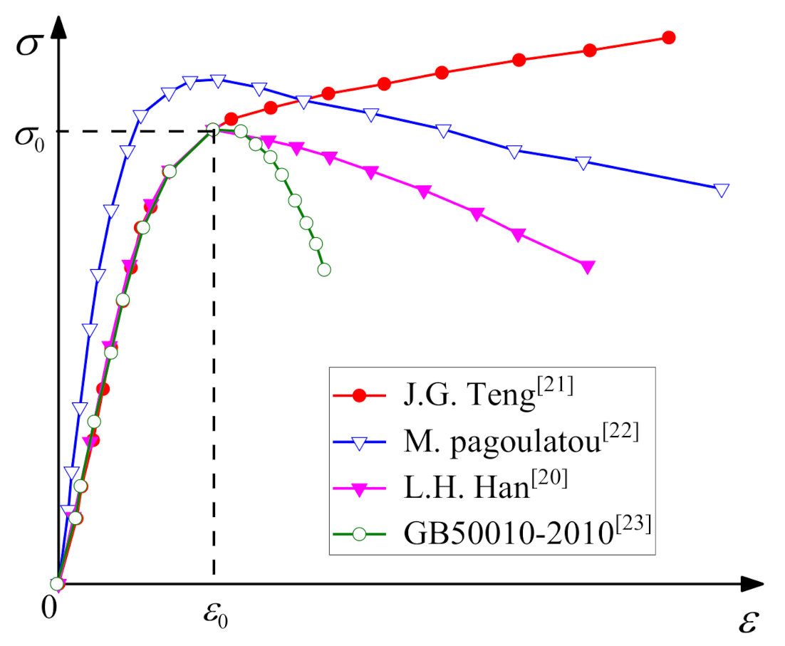
2.1.1. Constitutive Model of Concrete

Constitutive models of confined concrete have been proposed successively by Han [20], Teng [21], and Pagoulatou [22], and the constitutive model of unconfined concrete has been given in the Code for Design of Concrete Structures (GB50010-2010) [23]. The comparisons of different constitutive models are illustrated in Figure 1. Through comparative analysis, the constraint constitutive model proposed by Han is adopted as the constitutive model of concrete. The expressions are shown in Formulas (1)–(11), and the physical significance of each variable in the formula is shown in reference [20]. During finite element modeling, the plastic damage model of concrete is selected [24], which can take the stiffness degradation of concrete under low-cyclic loading into account.

The following formula represents the stress–strain curve of concrete subjected to uniaxial compression [20]:

$$y=\left\{\begin{array}{c}2·x-x^2 \left(x\le 1\right)\\ \frac{x}{{\beta }_0{\left(x-1\right)}^n+x} (x>1)\end{array}\right.$$

(1)

where:

$$x=\frac{\epsilon }{{\epsilon }_0}$$

(2)

$$y=\frac{\sigma }{{\sigma }_0}$$

(3)

$${\sigma }_0=f_c$$

(4)

$${\epsilon }_0={\epsilon }_{\mathrm{c}}+800·{\xi }^{0.2}·{10}^{-6}$$

(5)

$${\epsilon }_{\mathrm{c}}=\left(1300+12.5·f_{\mathrm{c}}\right)·{10}^{-6}$$

(6)

$$\eta \left\{\begin{array}{c}2 \left(circular \mathrm{steel} tube\right)\\ 1.6+\frac{1.5}{x} \left(\mathrm{Square} \mathrm{steel} tube\right)\end{array}\right.$$

(7)

$${\beta }_0\left\{\begin{array}{c}(2.36\times {10}^{-5}){}^{\left[0.25+{\left(\xi -0.5\right)}^7\right]}·f_c^{0.5}·0.5\ge 0.12 \left(circular \mathrm{steel} tube\right)\\ \frac{f_c^{0.1}}{1.2\sqrt{1+\xi }} \left(\mathrm{Square} \mathrm{steel} tube\right)\end{array}\right..$$

(8)

The following formula represents the stress–strain curve of concrete subjected to uniaxial tensile [20]:

$$y=\left\{\begin{array}{c}1.2·x-0.2·x^6 \left(x\le 1\right)\\ {\displaystyle \frac{x}{0.31·{\sigma }_P^2·{\left(x-1\right)}^{1.7}+x}} (x>1)\end{array}\right.$$

(9)

where $x=\frac{{\epsilon }_{\mathrm{c}}}{{\epsilon }_{\mathrm{P}}}$, $y=\frac{{\sigma }_{\mathrm{c}}}{{\sigma }_{\mathrm{P}}}$. ${\sigma }_{\mathrm{P}}$ denotes the peak tensile stress, ${\epsilon }_{\mathrm{P}}$ refers to the peak strain under tension, and these variables are calculated respectively according to the following formula:

$${\sigma }_{\mathrm{P}}=0.26\times {\left(1.25·f_{\mathrm{c}}\right)}^{2/3}$$

(10)

$${\epsilon }_{\mathrm{P}}=34.276\times {\sigma }_{\mathrm{P}}(\mu ·\epsilon ).$$

(11)

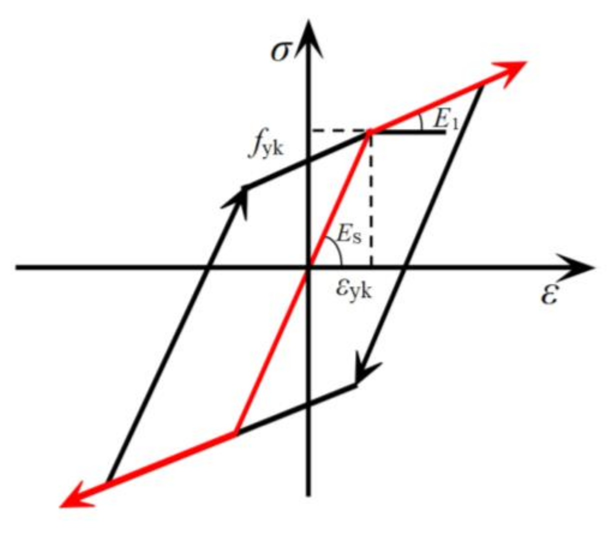
2.1.2. Constitutive Model of Steel

Considering the Baushenge effect [25], the constitutive model of steel adopts a double broken-line stress-hardening constitutive model. The expression is shown in Equation (12). The constitutive model is shown in Figure 2. The maximum plastic strain is 0.01, and the elastic modulus and Poisson’s ratio are 2.01 × 10⁵ Mpa and 0.3, respectively.

$$\sigma =\left\{\begin{array}{c}{E}_{\mathrm{s}}\epsilon \left(\epsilon \le {\epsilon }_{\mathrm{yk}}\right)\\ f_{\mathrm{yk}}+E_1\left(\epsilon -{\epsilon }_{\mathrm{yk}}\right) \left(\epsilon \ge {\epsilon }_{\mathrm{yk}}\right)\end{array}\right.$$

(12)

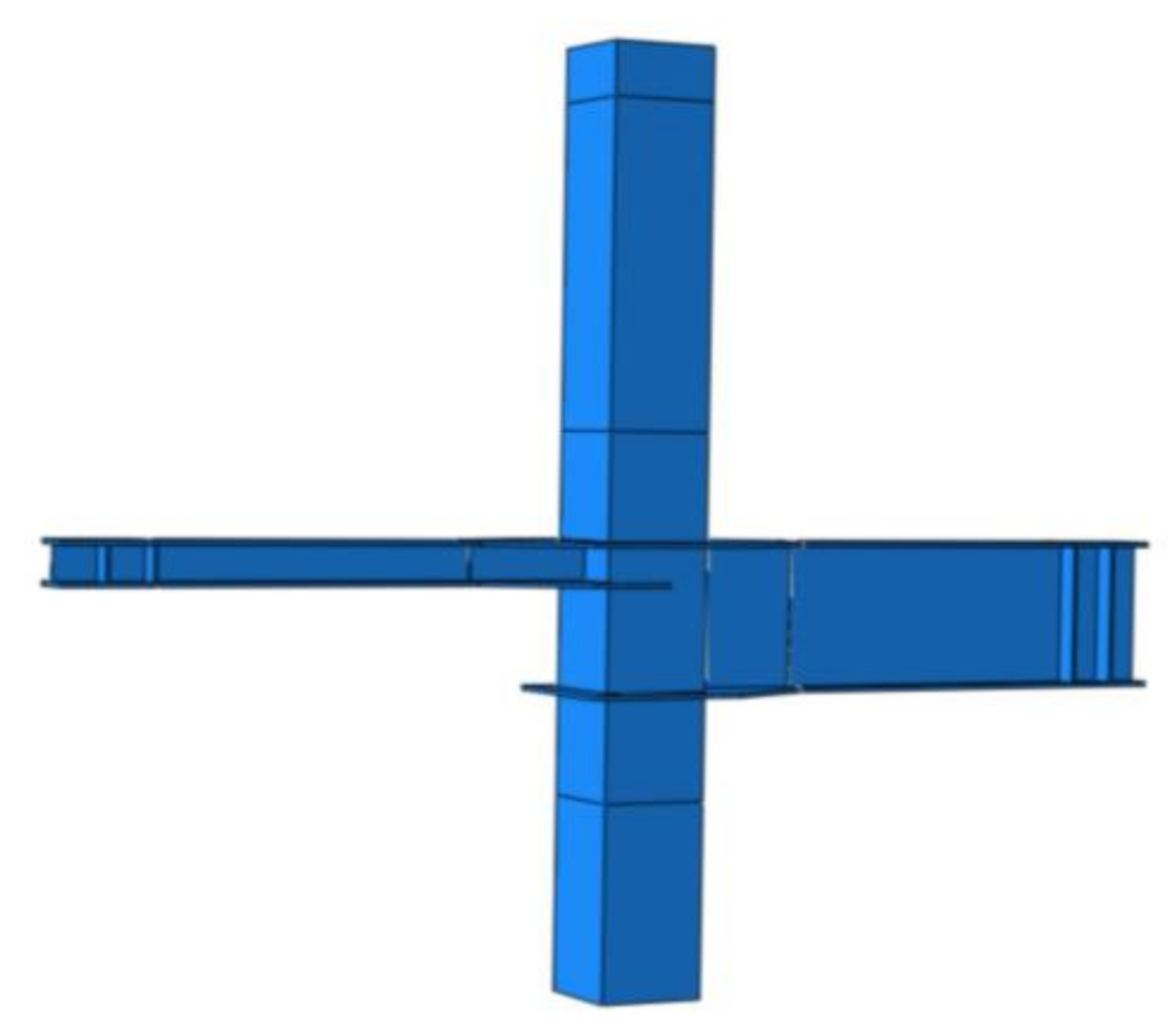
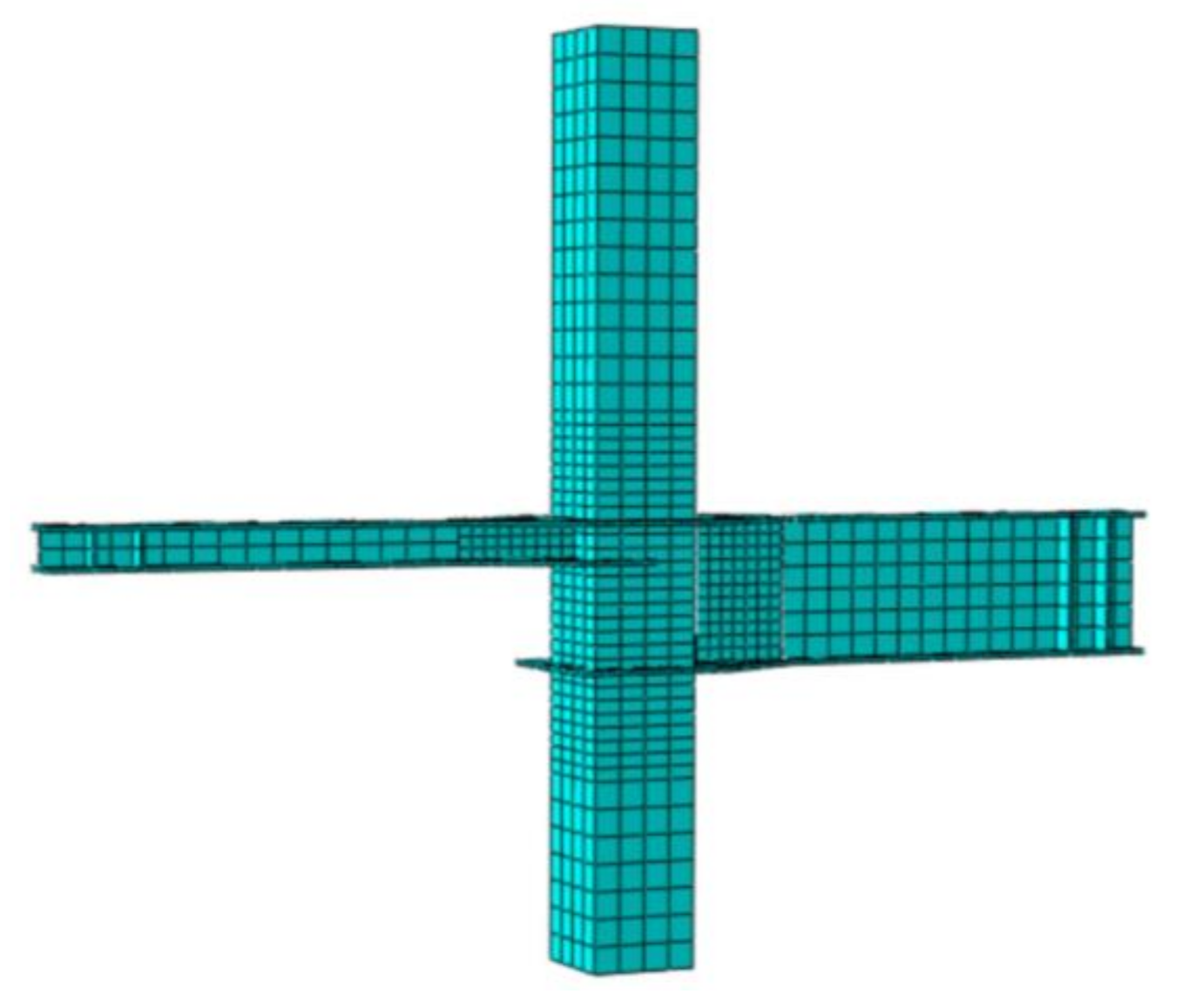
2.2. Finite Element Modeling

2.2.1. Establishment of Parts and Contact Mode

ABAQUS finite element software can accurately simulate the performance of engineering materials and has a great advantage in solving nonlinear problems. It can simulate the force and deformation of specimens ideally. Therefore, based on ABAQUS finite element software, this paper carries out a study on the seismic performance of the full-scale joints. Three-dimensional geometric models of square steel tubes, unequal height steel beams, and core confined concrete are created as shown in Figure 3. The eight-joint hexahedral element type C3D8H is used to simulate square steel tubes, unequal height steel beams, and core confined concrete [26,27]. The nonlinear symmetrical contact between the steel tube and concrete is simplified as normal hard contact and tangential friction contact. The outer wall of the steel tube and the ring plate, along with the ring plate and the beams, are bonded to simulate welding. In order to prevent flanges and webs from buckling, transverse stiffeners are set at the beam ends.

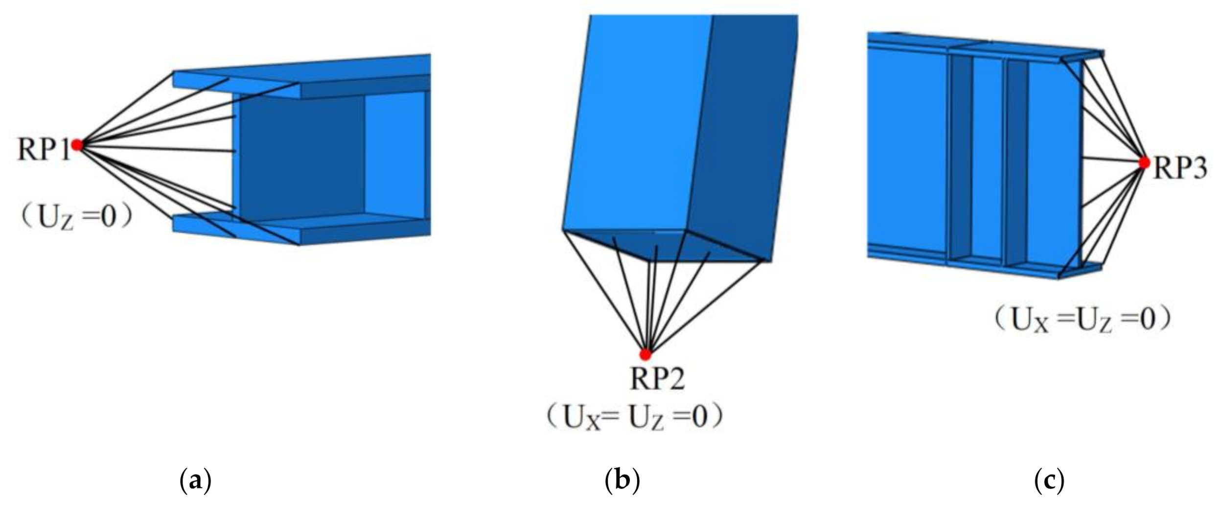
2.2.2. Boundary Conditions and Loading

According to the simplified calculation models of the joints, three reference points are set at the bottom of the columns and the two ends of the beams, namely RP1, RP2, and RP3. The reference points are respectively coupled with the bottom of the columns and the cross-section of the ends of the beams, and the hinge connection is achieved by using MPC to constrain the reference points. Vertical force and horizontal cyclic load are applied to the top of the columns, and the displacement and the rotation angle are not restricted. The displacement (U_Z) of the left ends for beams in the Z-direction is constrained by RP1, the displacements (U_X, U_Z) of the bottom ends for columns in the X and Z directions are constrained by RP2, and the displacements (U_X, U_Z) of the right ends for beams in the X and Z directions are constrained by RP3. The MPC constraint at the beam ends and column ends is shown in Figure 4.

3. Experimental Verification of Finite Element Model

3.1. Overview of Existing Test

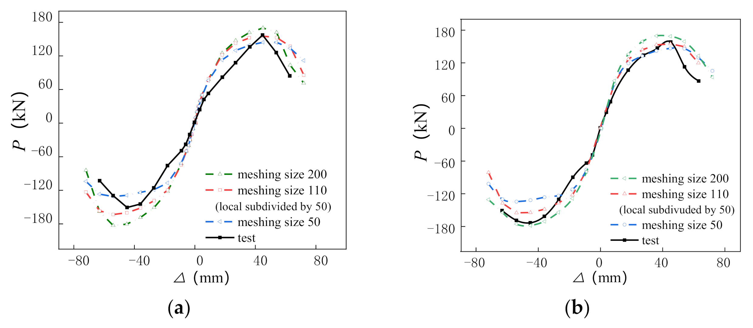
In order to verify the rationality of finite element models of full-scale composite joints with CFST columns and unequal high steel beams, four frame joints with concrete-filled steel square tubular columns and H-shaped unequal height steel beams according to the reduction ratio of 1:3 designed by Xu [19] were selected. The specific parameters of the four specimens are shown in

Table 1. Specific parameters of four specimens.

Specimen No.	I-Shaped High Steel Beam		I-Shaped Low Steel Beam		CFST Column
	Length l/mm	Section Size /mm4	Length l/mm	Section Size /mm4	Length l/mm	Section Size /mm3
CFSTJ-1	1010	280 × 100 × 6 × 8	1010	80 × 100 × 6 × 8	1735	200 × 200 × 6
CFSTJ-2				130 × 100 × 6 × 8
CFSTJ-3				180 × 100 × 6 × 8
CFSTJ-4				230 × 100 × 6 × 8

. The cubic compressive strength of concrete in the square steel tube is 40 Mpa. The yield strength and ultimate strength of the steel tube are 307 MPa and 419 MPa, respectively, and the yield strength and ultimate strength of the steel beams are 324 MPa and 439 MPa, respectively. The axial compression ratio of the columns is set as 0.4.

3.2. Mesh Division

Taking specimen CFSTJ-1 and specimen CFSTJ-2 as examples, the finite element models of different mesh sizes are established. The specimens are divided into three mesh sizes, namely 200 mm, 110 mm (50 mm is adopted as the size of meshing in joint domain), and 50 mm. The load–displacement skeleton curves of specimens with different mesh sizes can be obtained. The comparisons are shown in Figure 5. Through comparisons, the peak point of the skeleton curves obtained by the second meshing size coincides with the skeleton curves obtained by the test, which can prove that both are in good agreement. It can be seen that the simulation curves obtained by the second meshing size can better simulate the experimental situation, so this method is adopted to meshing. The mesh of the specimens is subdivided partially in the joint domain, as shown in Figure 6.

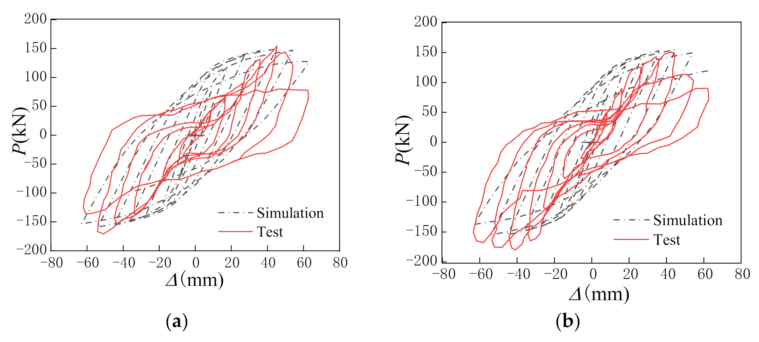
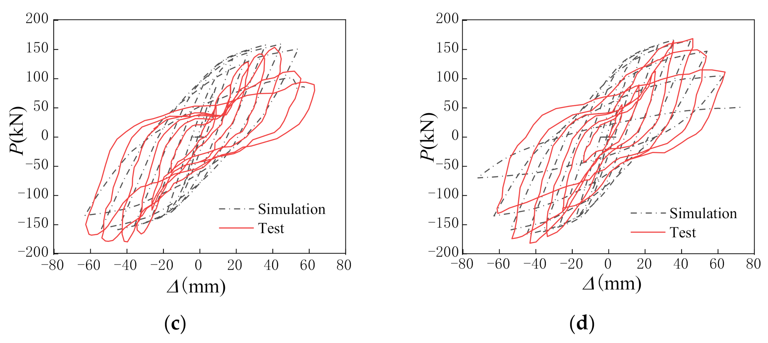
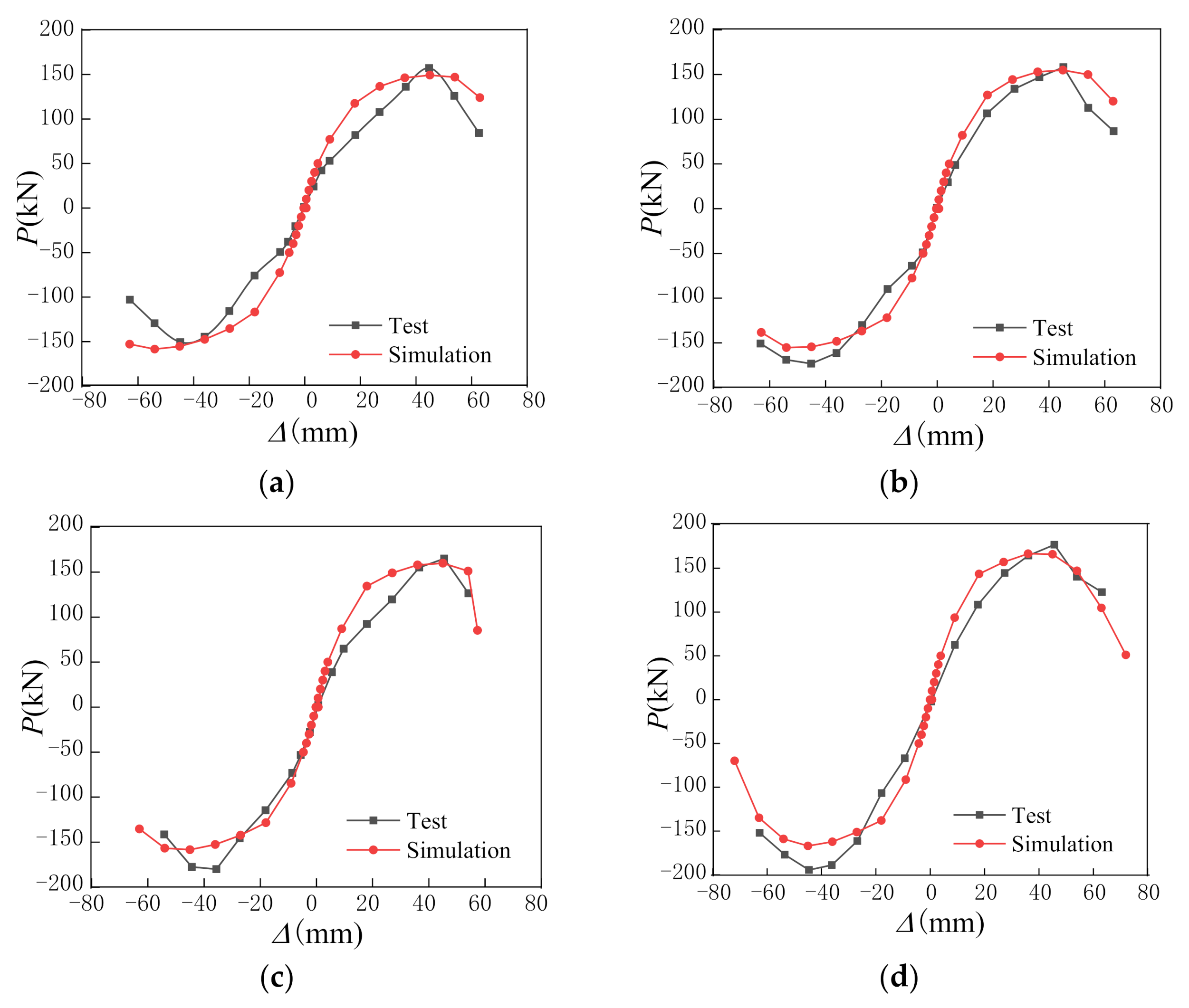
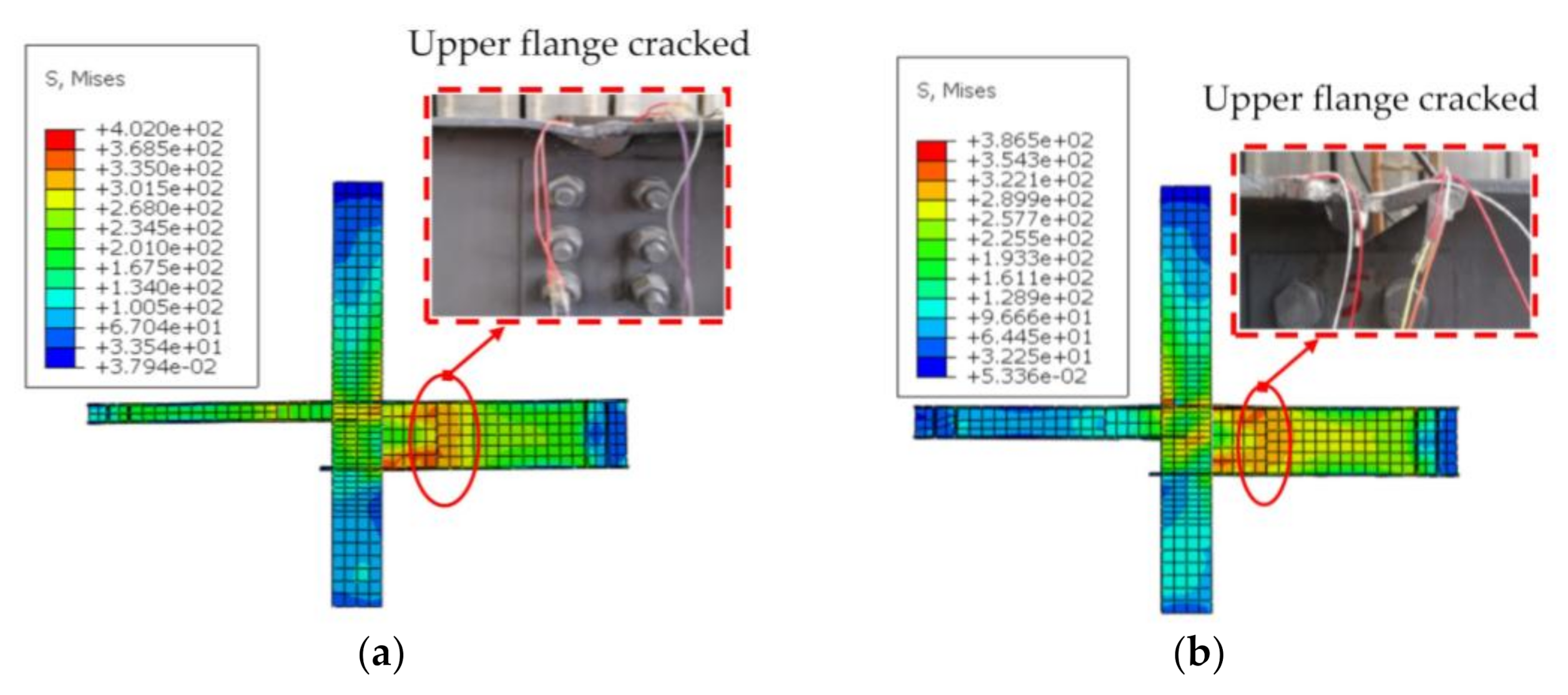
3.3. Comparison and Verification of Results

The above-mentioned meshing method is used to carry out finite element modeling and analysis, and the load–displacement hysteretic curves of the specimens are obtained, as shown in Figure 7. It can be seen from Figure 7 that the hysteresis curves are relatively full and have a certain pinching effect, which indicates that the specimens have strong energy dissipation capacity. The hysteresis curves obtained by simulations are in good agreement with the experimental hysteresis curves. The skeleton curves of the specimens extracted by the hysteresis curves are shown in Figure 8. It can be seen that the slopes of the skeleton curves obtained by the simulations are greater than the slopes of the skeleton curves obtained by the tests at the initial stage. It indicates that the initial stiffness of the skeleton curves obtained by the simulations are larger than the initial stiffness of the test skeleton curves. With the increasing of loading, the stiffness of the specimens gradually degrades. After the peak point of the curves, the load-bearing capacity of the specimens begins to decrease slowly. However, the ductility of the specimens is still good.

The test ultimate bearing capacity ($N_{\mathrm{t}}^{+}, N_{\mathrm{t}}^{-}$) and simulated ultimate bearing capacity ($N_{\mathrm{s}}^{+}, N_{\mathrm{s}}^{-}$) of the four specimens subjected to positive and negative loading can be obtained by skeleton curves, and the data are shown in

Table 2. Comparisons of ultimate bearing capacity between simulations and tests.

Specimen No.	${\mathit{N}}_{\mathbf{t}}^{+}$ /kN	${\mathit{N}}_{\mathbf{t}}^{-}$ /kN	$\overline{{\mathit{N}}_{\mathbf{t}}}$ /kN	${\mathit{N}}_{\mathbf{s}}^{+}$ /kN	${\mathit{N}}_{\mathbf{s}}^{-}$ /kN	$\overline{{\mathit{N}}_{\mathbf{s}}}$ /kN	$\left|\frac{\overline{{\mathit{N}}_{\mathbf{t}}}-\overline{{\mathit{N}}_{\mathbf{s}}}}{\overline{{\mathit{N}}_{\mathbf{t}}}}\right| \times 100\%$
CFSTJ-1	157.20	−150.62	153.91	149.23	−155.40	152.32	1.0%
CFSTJ-2	158.17	−173.20	165.69	154.98	−155.25	155.15	6.4%
CFSTJ-3	165.09	−180.02	172.56	159.93	−158.42	159.18	7.8%
CFSTJ-4	176.88	−194.39	185.64	166.63	−167.97	167.30	9.8%

. The mean value of the ultimate bearing capacity ($\overline{N_{\mathrm{t}}})$ obtained from the tests is compared with that of the ultimate bearing capacity ($\overline{N_{\mathrm{s}}}$) obtained from the simulations, and the maximum error is 9.8%, which can meet the accuracy requirements of engineering. The rationality and accuracy of the finite element models are verified. The stress cloud diagram of the models and failure modes of tests are shown in Figure 9.

4. Parameter Analysis

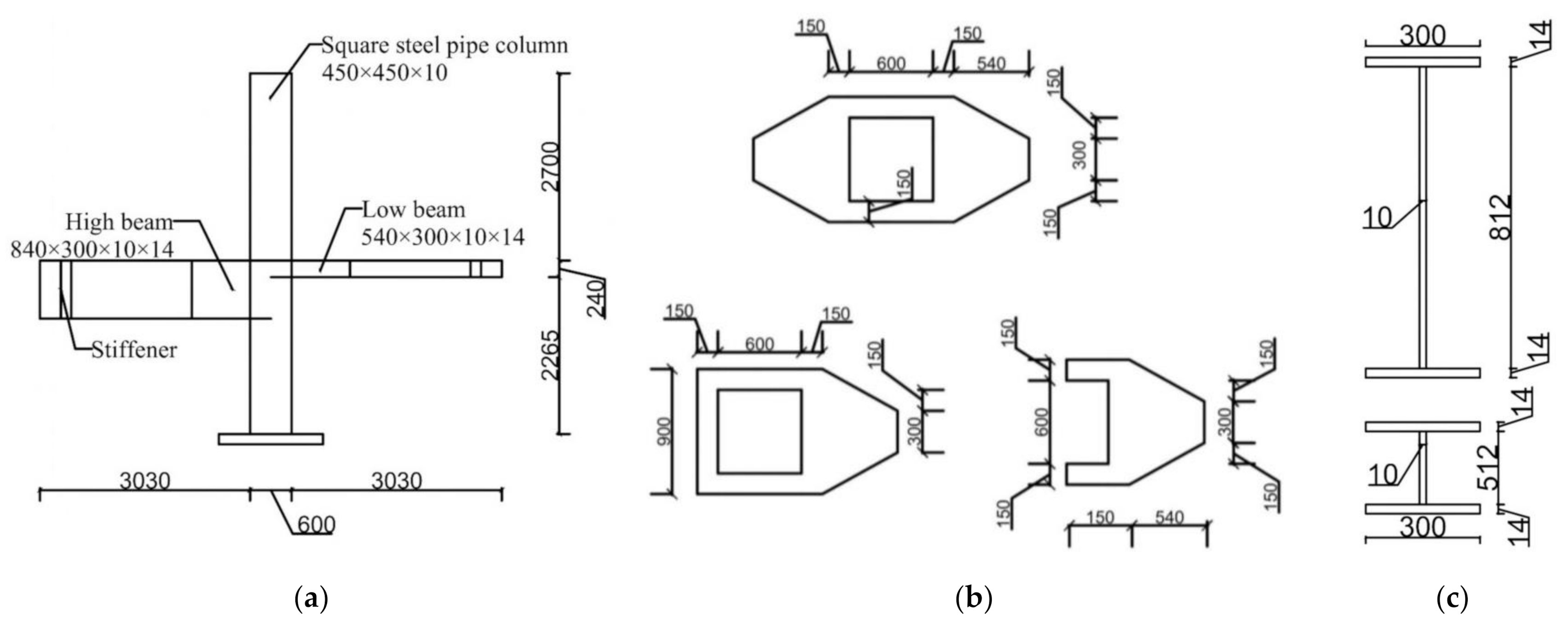
4.1. Design of Full-Scale Specimens

In order to study the seismic behavior of full-scale asymmetrical composite joints with CFST columns and unequal high steel beams, 36 joints are designed with a CFST hoop coefficient (ξ), axial compression ratio (n₀), compressive strength of cubic concrete (f_cuk), strength of steel tubes (f_yk), and cross-sectional size of beams and columns as the main control parameters. The specific parameters of the specimens are shown in

Table 3. Parameters of specimens.

Specimen No.	D /mm2	t /mm	fcuk /MPa	fyk /MPa	ξ	n0	h1 × b1 × t1 × t2 /mm4	h2× b2× t3× t4 /mm4
J1	450 × 450	10	40	235	0.559	0.2	840 × 300 × 10 × 14	540 × 300 × 10 × 14
J2	500 × 500	10	40	235	0.500	0.2	840 × 300 × 10 × 14	540 × 300 × 10 × 14
J3	550 × 550	10	40	235	0.452	0.2	840 × 300 × 10 × 14	540 × 300 × 10 × 14
J4	600 × 600	10	40	235	0.412	0.2	840 × 300 × 10 × 14	540 × 300 × 10 × 14
J5	500 × 500	10	30	235	0.666	0.2	840 × 300 × 10 × 14	540 × 300 × 10 × 14
J6	500 × 500	10	50	235	0.400	0.2	840 × 300 × 10 × 14	540 × 300 × 10 × 14
J7	500 × 500	10	60	235	0.333	0.2	840 × 300 × 10 × 14	540 × 300 × 10 × 14
J8	500 × 500	10	70	235	0.286	0.2	840 × 300 × 10 × 14	540 × 300 × 10 × 14
J9	500 × 500	10	80	235	0.250	0.2	840 × 300 × 10 × 14	540 × 300 × 10 × 14
J10	500 × 500	8	40	235	0.395	0.2	840 × 300 × 10 × 14	540 × 300 × 10 × 14
J11	500 × 500	12	40	235	0.607	0.2	840 × 300 × 10 × 14	540 × 300 × 10 × 14
J12	500 × 500	14	40	235	0.718	0.2	840 × 300 × 10 × 14	540 × 300 × 10 × 14
J13	500 × 500	16	40	235	0.831	0.2	840 × 300 × 10 × 14	540 × 300 × 10 × 14
J14	500 × 500	16	40	235	0.500	0.1	840 × 300 × 10 × 14	540 × 300 × 10 × 14
J15	500 × 500	16	40	235	0.500	0.3	840 × 300 × 10 × 14	540 × 300 × 10 × 14
J16	500 × 500	16	40	235	0.500	0.4	840 × 300 × 10 × 14	540 × 300 × 10 × 14
J17	500 × 500	16	40	235	0.500	0.5	840 × 300 × 10 × 14	540 × 300 × 10 × 14
J18	500 × 500	16	40	235	0.500	0.6	840 × 300 × 10 × 14	540 × 300 × 10 × 14
J19	500 × 500	10	40	235	0.500	0.2	800 × 300 × 10 × 14	540 × 300 × 10 × 14
J20	500 × 500	10	40	235	0.500	0.2	760 × 300 × 10 × 14	540 × 300 × 10 × 14
J21	500 × 500	10	40	235	0.500	0.2	720 × 300 × 10 × 14	540 × 300 × 10 × 14
J22	500 × 500	10	40	235	0.500	0.2	680 × 300 × 10 × 14	540 × 300 × 10 × 14
J23	500 × 500	10	40	235	0.500	0.2	840 × 300 × 10 × 14	460 × 300 × 10 × 14
J24	500 × 500	10	40	235	0.500	0.2	840 × 300 × 10 × 14	420 × 300 × 10 × 14
J25	500 × 500	10	40	235	0.500	0.2	840 × 300 × 10 × 14	380 × 300 × 10 × 14
J26	500 × 500	10	40	345	0.734	0.2	840 × 300 × 10 × 14	540 × 300 × 10 × 14
J27	500 × 500	10	40	490	1.042	0.2	840 × 300 × 10 × 14	540 × 300 × 10 × 14
J28	500 × 500	10	40	630	1.340	0.2	840 × 300 × 10 × 14	540 × 300 × 10 × 14
J29	500 × 500	10	40	235	0.500	0.2	840 × 300 × 10 × 14	540 × 300 × 8 × 14
J30	500 × 500	10	40	235	0.500	0.2	840 × 300 × 10 × 14	540 × 300 × 12 × 14
J31	500 × 500	10	40	235	0.500	0.2	840 × 300 × 10 × 14	540 × 300 × 14 × 14
J32	500 × 500	10	40	235	0.500	0.2	840 × 300 × 10 × 14	540 × 300 × 16 × 14
J33	500 × 500	10	40	235	0.500	0.2	840 × 300 × 10 × 14	540 × 300 × 10 × 10
J34	500 × 500	10	40	235	0.500	0.2	840 × 300 × 10 × 14	540 × 300 × 10 × 12
J35	500 × 500	10	40	235	0.500	0.2	840 × 300 × 10 × 14	540 × 300 × 10 × 16
J36	500 × 500	10	40	235	0.500	0.2	840 × 300 × 10 × 14	540 × 300 × 10 × 18

Note: D is the dimension of the concrete-filled square steel tube column; t is the wall thickness of the square steel tube; f_cuk and f_yk are the standard values of the concrete cube compressive strength and steel tube yield strength, respectively. ξ is the hoop coefficient; n₀ is the axial compression ratio; h₁, b₁, t₁, and t₂ are the height, flange width, web thickness, and flange thickness of the high beam, respectively. h₂, b₂, t₃ and t₄ are the height, flange width, web thickness, and flange thickness of the low beam, respectively.

, and the specific size of specimen J1 is shown in Figure 10. The length of the column is 5205 mm, and the length of the beam is 3030 mm. The steel beam adopts H-shaped welded steel beam. Transverse stiffeners are installed near the ends of the simply-supported beams to improve the overall stability of the beams. To ensure the reliable connection between the ends of beams and columns, the annular enclosed connecting plate is adopted as the upper flange of the beam end, while the lower flange adopts the open connecting plate.

4.2. The Main Parametric Analysis

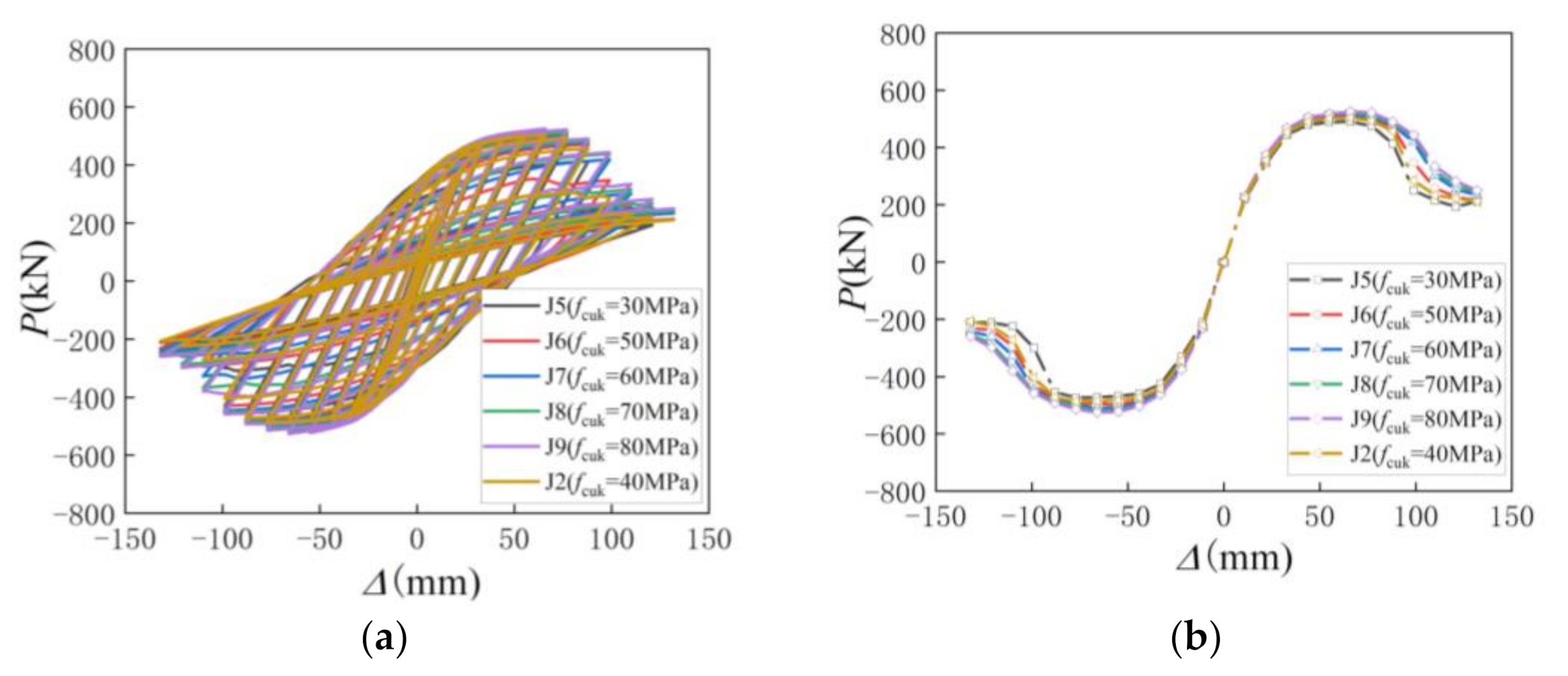
4.2.1. Compressive Strengths of Concrete Cubes (f_cuk)

The hysteresis curves and skeleton curves with different f_cuk are shown in Figure 11. The peak load (P_max) and ultimate load (P_u) of the specimens are shown in

Table 4. Load, displacement, and ductility coefficients of the specimens at each stage.

Specimen No.	fcuk /MPa	Pmax /kN	Δmax /mm	Py /kN	Δy /mm	Pu /kN	Δu /mm	μ
J2	30	503.38	60.74	438.71	31.60	402.04	91.24	2.89
J5	40	490.20	59.10	458.63	35.57	394.07	90.29	2.54
J6	50	509.77	54.79	448.67	31.87	408.95	94.25	2.96
J7	60	517.57	62.59	450.48	31.74	413.62	99.18	3.12
J8	70	521.85	65.94	450.93	30.98	417.98	101.09	3.26
J9	80	525.44	69.56	448.22	30.71	423.41	101.03	3.29

. It can be found from Figure 11 and Table 4 that with the increasing of f_cuk, the peak load (P_max) of the specimens gradually increases. The f_cuk increases from 30 to 40 Mpa, 50 Mpa, 60 Mpa, 70 Mpa and 80 Mpa in turn, and the P_max of the specimen increases from 490.196 to 503.375 kN, 509.765 kN, 517.574 kN, 521.854 kN, and 525.442 kN, which increases by 2.69%, 4.00%, 5.59%, 6.46%, and 7.19%, respectively. When f_cuk exceeds 60 Mpa, the increasing of P_max is no longer obvious. It can be seen that the restraint effect of steel tubes on ordinary concrete is significant, but the restraint effect on high-strength concrete is not obvious.

Ductility is one of the important indicators of the seismic performance of the specimens, which can reflect the stiffness, bearing capacity, and energy dissipation of the specimens. It is represented by the ductility coefficient (μ), and the expression is shown in Formula (13).

μ = Δ_u/Δ_y

(13)

where Δ_u refers to the ultimate displacement and Δ_y denotes the yield displacement.

In this paper, the Park method [28] is adopted to calculate the equivalent yield point of the specimens, as shown in Figure 12. Based on the P-Δ curves, the equivalent yield point can be obtained by finding the corresponding point of 0.7 times as P_max on the curves, and the yield load (P_y) can be calculated, as shown in Table 4. The peak displacement (Δ_max), yield displacement, ultimate displacement, and the ductility coefficient of the specimens are shown in Table 4. With the increasing of f_cuk, μ gradually increases. When the f_cuk increases from 30 to 40 Mpa, 50 Mpa, 60 Mpa, 70 Mpa, and 80 Mpa in turn, μ increases from 2.54 to 2.89, 2.96, 3.12, 3.26, and 3.29, which increases by 13.78%, 16.54%, 22.83%, 28.35%, and 29.53%, respectively. It can be found that f_cuk has a significant effect on the ductility of specimens.

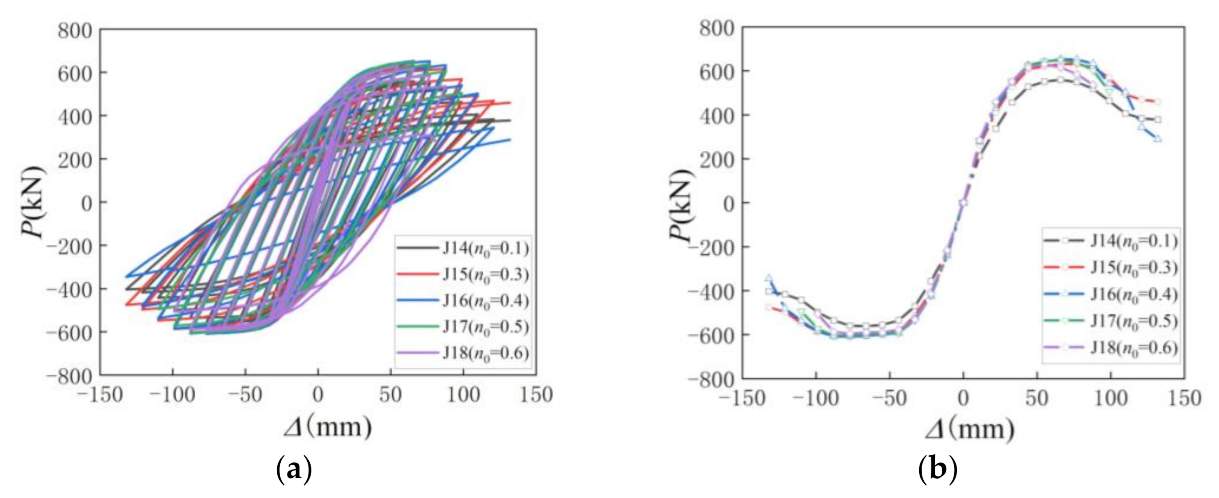
4.2.2. Axial Compression Ratios (n₀)

The hysteresis curves and skeleton curves of the specimens with different n₀ are shown in Figure 13. The load, displacement, and ductility coefficients of the specimens at each stage are shown in

Table 5. Load, displacement, and ductility coefficients of the specimens at each stage.

Specimen No.	n0	Pmax /kN	Δmax /mm	Py /kN	Δy /mm	Pu /kN	Δu /mm	μ
J14	0.1	558.98	66.14	492.59	38.30	444.78	101.85	2.66
J15	0.3	630.92	66.42	548.73	36.43	504.90	107.07	2.94
J16	0.4	652.91	66.01	563.21	34.57	521.93	104.31	3.02
J17	0.5	648.94	66.07	547.39	33.83	519.02	96.40	2.85
J18	0.6	630.45	55.06	529.26	32.44	501.64	90.48	2.79

. It can be seen from Figure 13 and Table 5 that with the increasing of n₀, the P_max of the specimens gradually increases firstly and then gradually decreases after reaching a peak point. When n₀ increases from 0.1 to 0.3 and 0.4, the P_max of the specimens increases from 558.98 to 630.92 kN and 652.91 kN, which increases by 12.87% and 16.81%, respectively. When n₀ increases from 0.4 to 0.5 and 0.6, the P_max of the specimens decreases from 652.91 to 648.94 kN and 630.45 kN, which decreases by 0.60% and 3.44%, respectively. It can be seen that the axial compression ratio has a significant effect on the P_max of the specimens. When the axial compression ratio is controlled as the value of 0.4, the load-bearing capacity of the specimens reaches maximum. When n₀ increases from 0.1 to 0.3 and 0.4, the μ of the specimens increases from 2.66 to 2.94 and 3.02, which increases by 10.53% and 13.53%, respectively. When n₀ increases from 0.4 to 0.5 and 0.6, the μ of the specimens decreases from 3.02 to 2.85 and 2.79, which decreases by 5.63% and 7.62%, respectively. It can be seen that the axial compression ratio has a significant effect on the ductility of the specimens. When the axial compression ratio is not more than 0.4, the ductility of the specimens can be maintained above 3, which indicates the asymmetrical composite joint has good deformability.

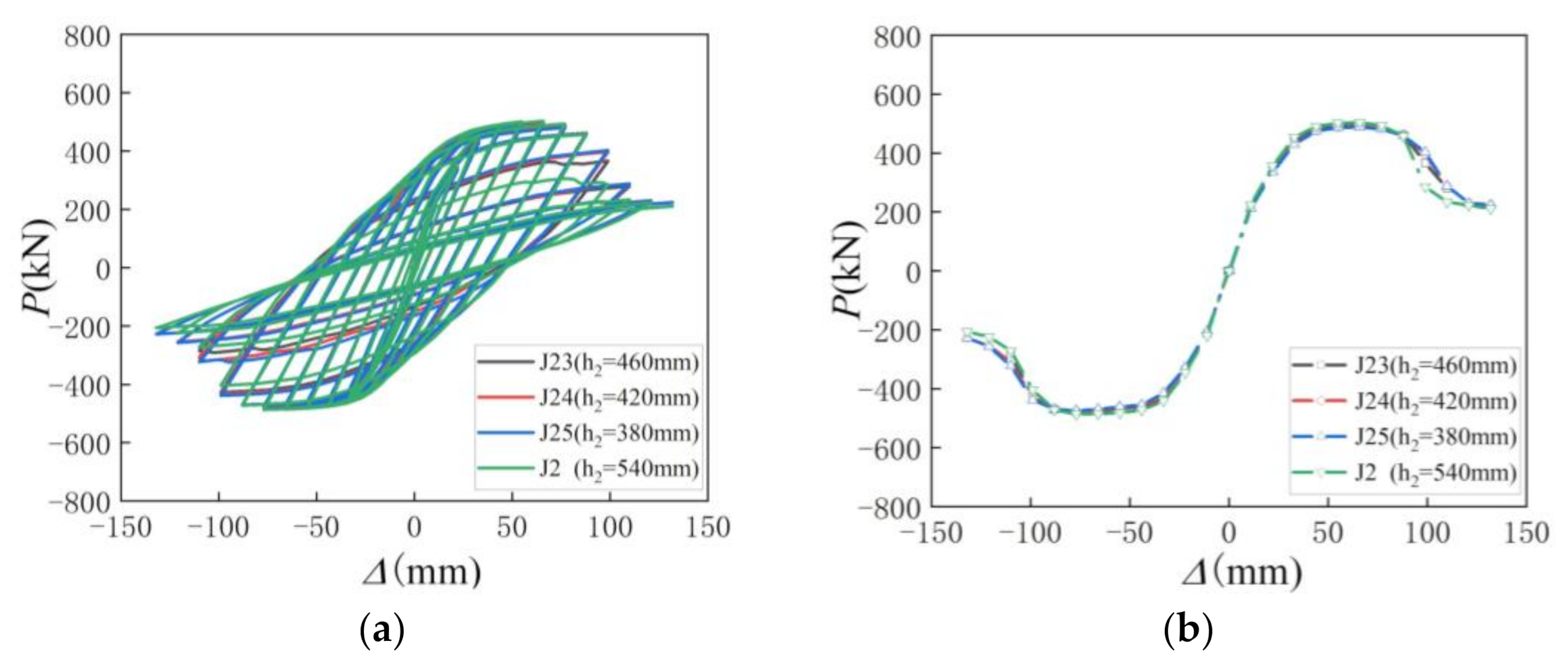
4.2.3. The Heights of the Low Beams (h₂)

The hysteretic curves and skeleton curves of specimens with different h₂ are shown in Figure 14. Load, displacement, and ductility coefficients of specimens at each stage are shown in

Table 6. Load, displacement, and ductility coefficients of the specimens at each stage.

Specimen No.	h2 /mm	Pmax /kN	Δmax /mm	Py /kN	Δy /mm	Pu /kN	Δu /mm	μ
J23	460	494.58	66.07	438.37	32.96	395.25	95.68	2.90
J24	420	491.28	66.23	427.16	33.20	392.26	98.39	2.96
J25	380	488.20	60.25	432.94	33.99	390.56	101.19	2.98
J2	540	503.38	60.74	438.71	31.60	402.04	91.24	2.89

. It can be seen from Figure 14 and Table 6 that when h₂ increases from 380 to 420 mm, 460 mm, and 540 mm, the P_max of the specimens increases from 488.20 to 491.28 kN, 494.58 kN, and 503.38 kN, which increases by 0.63%, 1.31%, and 3.11%, respectively. It can be found that with the increasing of h₂, the P_max of the specimens is not improved significantly. Table 6 shows that the height of the low beams has no significant influence on the ductility of the specimens.

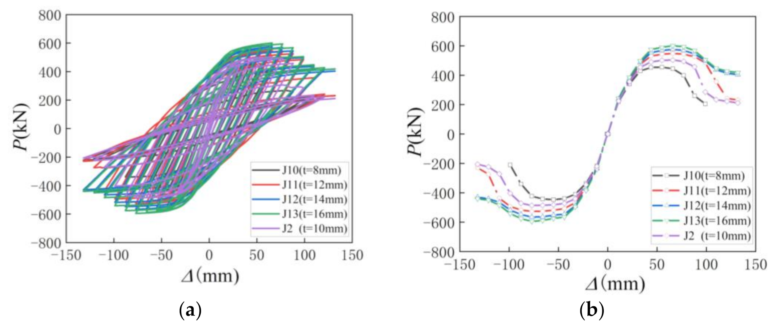
4.2.4. Wall Thicknesses of Square Steel Tubes (t)

The hysteresis curves and skeleton curves of the specimens with different t are shown in Figure 15, and the load, displacement, and ductility coefficients of the specimens at each stage are shown in

Table 7. Load, displacement, and ductility coefficients of the specimens at each stage.

Specimen No.	t4 /mm	Pmax /kN	Δmax /mm	Py /kN	Δy /mm	Pu /kN	Δu /mm	μ
J2	10	503.38	60.74	438.71	31.60	402.04	91.24	2.89
J10	8	454.53	50.75	390.27	28.18	362.92	79.96	2.84
J11	12	547.97	65.80	477.65	34.47	435.36	102.74	2.98
J12	14	575.80	66.07	507.07	35.18	461.07	106.06	3.01
J13	16	600.86	66.21	546.01	34.74	479.91	105.33	3.03

. It can be seen from Figure 15 that when t of the specimens increases from 8 to 10 mm, 12 mm, 14 mm, and 16 mm, P_max of the specimens increases from 454.53 to 503.38 kN, 547.97 kN, 575.80 kN, and 600.86 kN in turn, which increases by 10.75%, 20.56%, 26.68%, and 32.19%, respectively. It can be seen that with the increasing of t, the constraint effect of steel tubes is enhanced, and the P_max of specimens is improved more significantly. When the t of the specimens increases from 8 to 10 mm, 12 mm, 14 mm, and 16 mm, the μ of the specimens increases from 2.84 to 2.89, 2.98, 3.01, and 3.03 in turn, which increases by 1.76%, 4.93%, 5.65%, and 6.69%, respectively. It can be seen that with the increasing of t, the ductility of the specimens gradually increases, but t has no significant influence on the ductility of the specimens. When the wall thickness of square steel tubes is no less than 14 mm, the ductility of the specimens can be kept above 3, and the composite joints have good deformation ability.

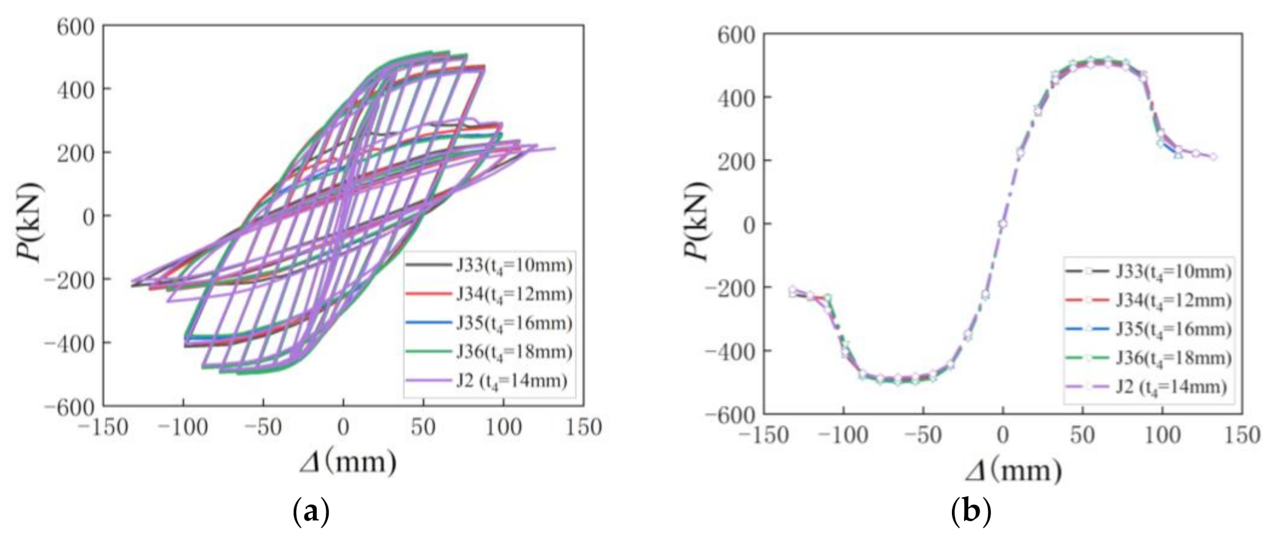
4.2.5. Flange Thicknesses of Low Beams (t₄)

The hysteretic curves and P-Δ skeleton curves of the specimens with different t₄ are shown in Figure 16. The load, displacement, and ductility coefficients of the specimens at each stage are shown in

Table 8. Load, displacement, and ductility coefficients of specimens at each stage.

Specimen No.	t4 /mm	Pmax /kN	Δmax /mm	Py /kN	Δy /mm	Pu /kN	Δu /mm	μ
J2	14	503.38	60.74	438.71	31.60	402.04	91.24	2.89
J33	10	503.05	56.86	462.14	35.96	402.44	92.50	2.57
J34	12	511.08	59.37	459.42	33.79	408.86	91.72	2.71
J35	16	516.44	61.97	457.04	31.02	413.15	89.60	2.89
J36	18	516.90	58.66	477.76	31.41	413.52	91.80	2.92

. As we can see from Figure 16 and Table 8, when t₄ increases from 10 to 12 mm, 14 mm, 16 mm, and 18 mm in turn, the P_max of the specimens increases from 503.05 to 511.08 kN, 503.38 kN, 516.44 kN, and 516.90 kN, respectively, indicating little influence on the P_max of specimens. When t₄ increases from 10 to 12 mm, 14 mm, 16 mm, and 18 mm in turn, the μ of the specimens increases by 5.44%, 12.45%, 12.45%, and 13.62%, respectively. It can be seen that with the increasing of t₄, the ductility of the specimens gradually increases.

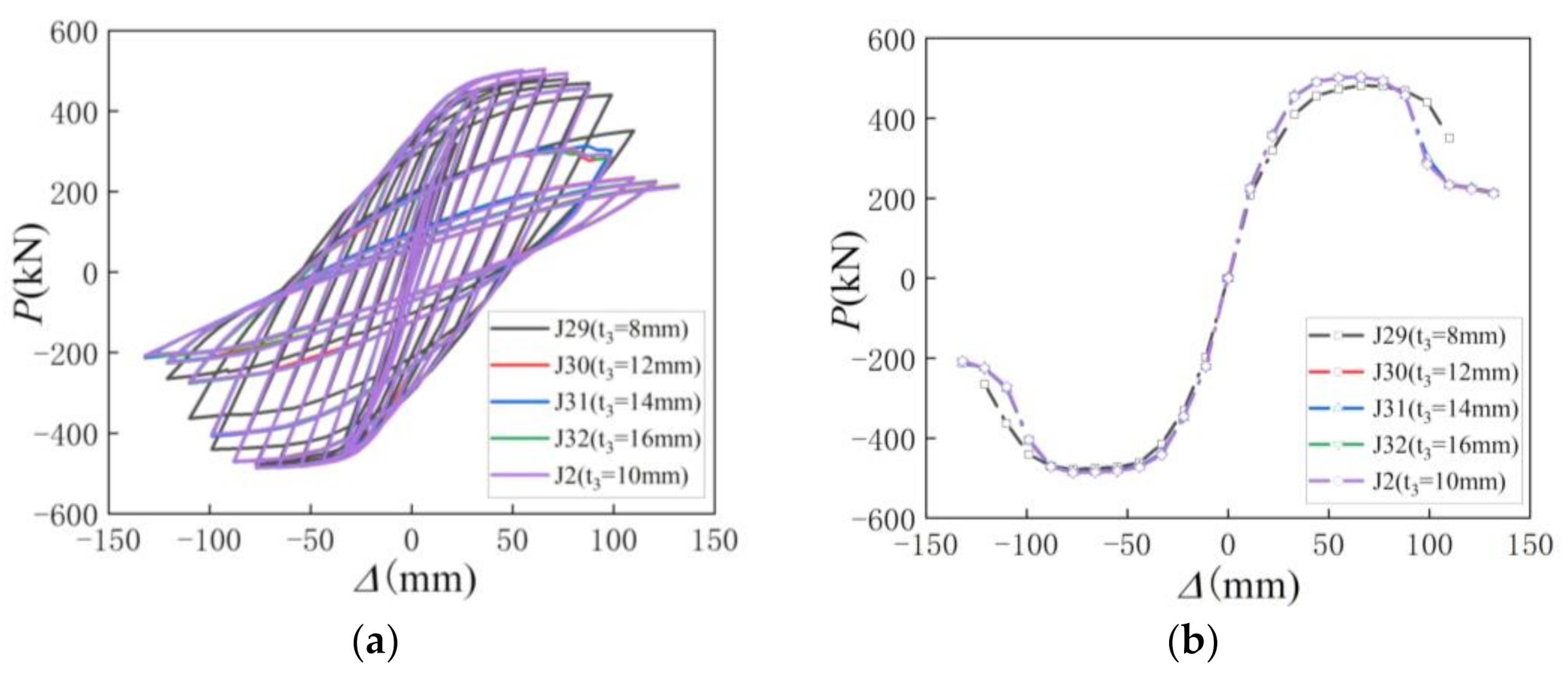
4.2.6. Web Thicknesses of Low Beams (t₃)

The hysteretic curves and P-Δ skeleton curves of the specimens with different t₃ are shown in Figure 17. The load, displacement, and ductility coefficients of the specimens at each stage are shown in

Table 9. Load, displacement, and ductility coefficients of specimens at each stage.

Specimen No.	t3 /mm	Pmax /kN	Δmax /mm	Py /kN	Δy /mm	Pu /kN	Δu /mm	μ
J2	10	503.38	60.74	438.71	31.60	402.04	91.24	2.89
J29	8	482.19	67.37	430.56	38.03	385.75	110.27	2.90
J30	12	503.76	60.94	420.71	31.07	403.00	91.18	2.93
J31	14	503.41	61.42	444.14	31.20	402.73	91.72	2.94
J32	16	503.52	58.28	446.52	31.67	402.82	91.72	2.90

. As we can see from Figure 17 and Table 9, when t₃ increases from 8 to 10 mm, 12 mm, 14 mm, and 16 mm in turn, the P_max of the specimens increases from 482.19 to 503.38 kN, 503.76 kN, 503.41 kN, and 503.52 kN, which increases by 4.39%, 4.47%, 4.40%, and 4.42%, respectively. It can be seen that t₃ has little influence on the P_max and μ of the specimens.

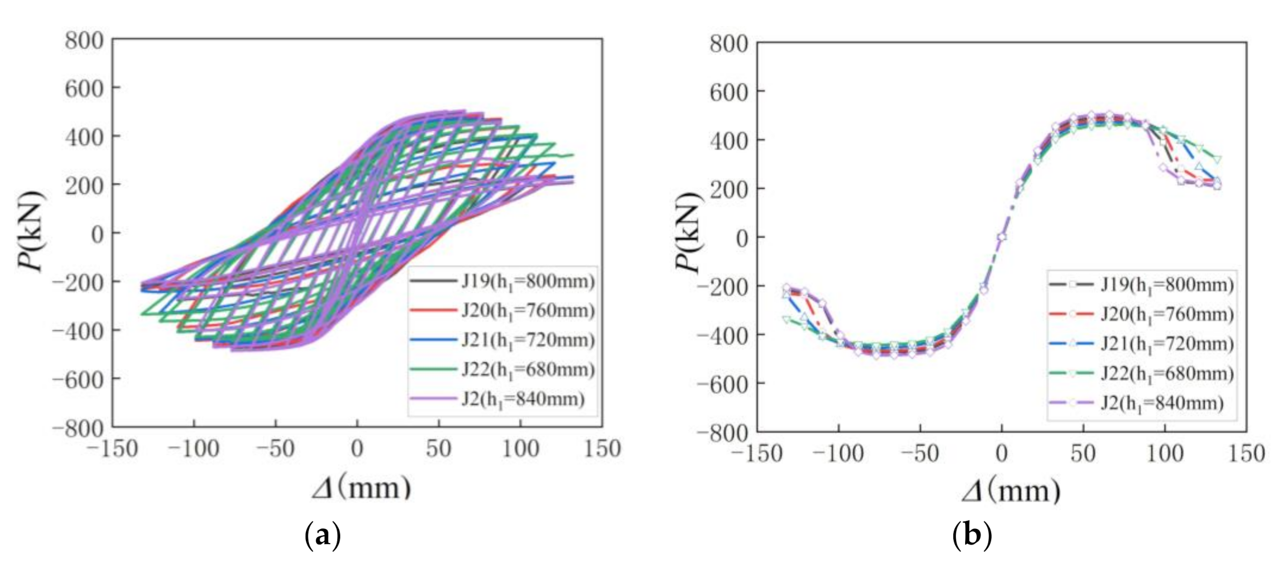
4.2.7. The Heights of the High Beams (h₁)

The hysteresis curves and P-Δ skeleton curves of specimens with different h₁ are shown in Figure 18. The load, displacement, and ductility coefficients of specimens at each stage are shown in

Table 10. Load, displacement, and ductility coefficients of the specimens at each stage.

Specimen No.	h1 /mm	Pmax /kN	Δmax /mm	Py /kN	Δy /mm	Pu /kN	Δu /mm	μ
J2	840	503.38	60.74	437.35	31.60	402.04	91.24	2.89
J19	800	491.89	66.01	437.35	32.76	391.90	98.50	3.01
J20	760	483.67	66.35	428.30	33.65	385.38	101.92	3.03
J21	720	472.88	66.31	416.98	33.91	376.22	111.80	3.30
J22	680	460.77	70.78	404.75	33.91	368.35	119.70	3.53

. As we can see from Figure 18 and Table 10, when h₁ decreases from 840 to 800 mm, 760 mm, 720 mm, and 680 mm in turn, the P_max of the specimens decreases from 503.38 to 491.89 kN, 483.67 kN, 472.88 kN, and 460.77 kN, which decreases by 2.28%, 3.91%, 6.06%, and 8.46%, respectively. It can be seen that with the decreasing of h₁, the P_max of specimens gradually decrease, and the descending branch of the skeleton curves slow down. When h₁ decreases from 840 to 800 mm, 760 mm, 720 mm, and 680 mm, in turn, μ increases from 2.89 to 3.01, 3.03, 3.30, and 3.53, which increases by 4.15%, 4.84%, 14.19%, and 22.15%, respectively. It can be seen that with the decreasing of h₁, the ductility of the specimens gradually increases. The descending branch of skeleton curves for each specimen is relatively gentle, which indicates that although the weld bead cracks at a later stage, the specimen still has good bearing capacity. When the height of the high beam is less than 800 mm, the ductility of the specimens can be kept above 3, and the composite joints have good deformation ability.

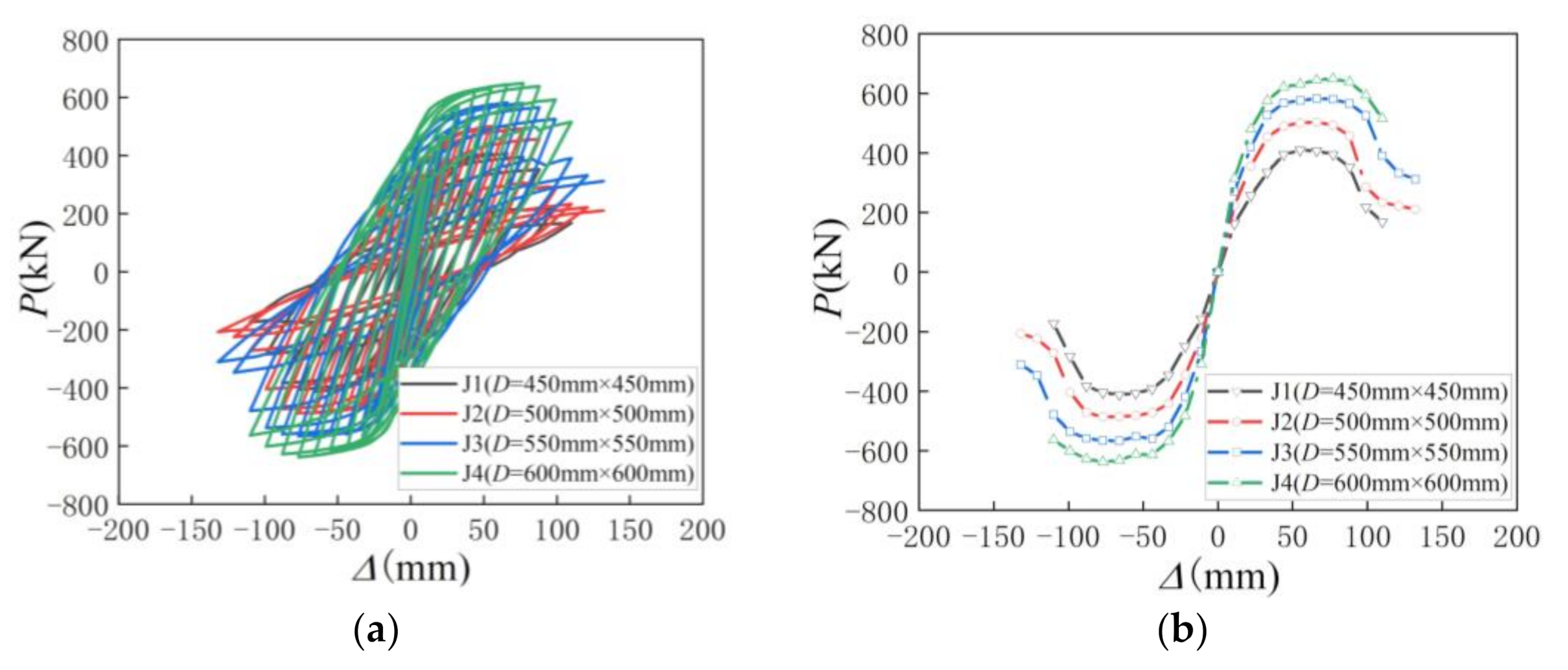
4.2.8. Cross-Sectional Sizes of Square Steel Tubes (D)

The hysteresis curves and P-Δ skeleton curves of specimens with different D are shown in Figure 19. The load, displacement, and ductility coefficients of the specimens at each stage are shown in

Table 11. Load, displacement, and ductility coefficients of the specimens at each stage.

Specimen No.	D /mm	Pmax /kN	Δmax /mm	Py /kN	Δy /mm	Pu /kN	Δu /mm	μ
J1	450 × 450	408.713	55.06	365.7	37.96	330.05	90.08	2.37
J2	500 × 500	503.375	60.74	438.71	31.6	402.04	91.24	2.89
J3	550 × 550	582.66	66.47	493.2	29.61	466.51	104.06	3.51
J4	600 × 600	649.29	75.1	551.44	30.44	518.66	108.82	3.57

. It can be seen from Figure 19 and Table 11 that when D increases from 450 mm × 450 mm to 500 mm × 500 mm, 550 mm × 550 mm, and 600 mm × 600 mm in turn, the P_max of the specimens increase from 408.71 to 503.38 kN, 582.66 kN, and 649.29 kN, which increases by 23.16%, 45.56%, and 58.86%, respectively. It can be seen that with the increasing of D, the P_max of specimens increase significantly. When D increases from 450 mm × 450 mm to 500 mm × 500 mm, 550 mm × 550 mm, and 600 mm × 600 mm in turn, the μ of the specimens increases from 2.37 to 2.89, 3.51, and 3.57, which increases by 21.94%, 48.10%, and 50.63% respectively. It can be seen that with the increasing of D, the ductility of the specimens gets better and better.

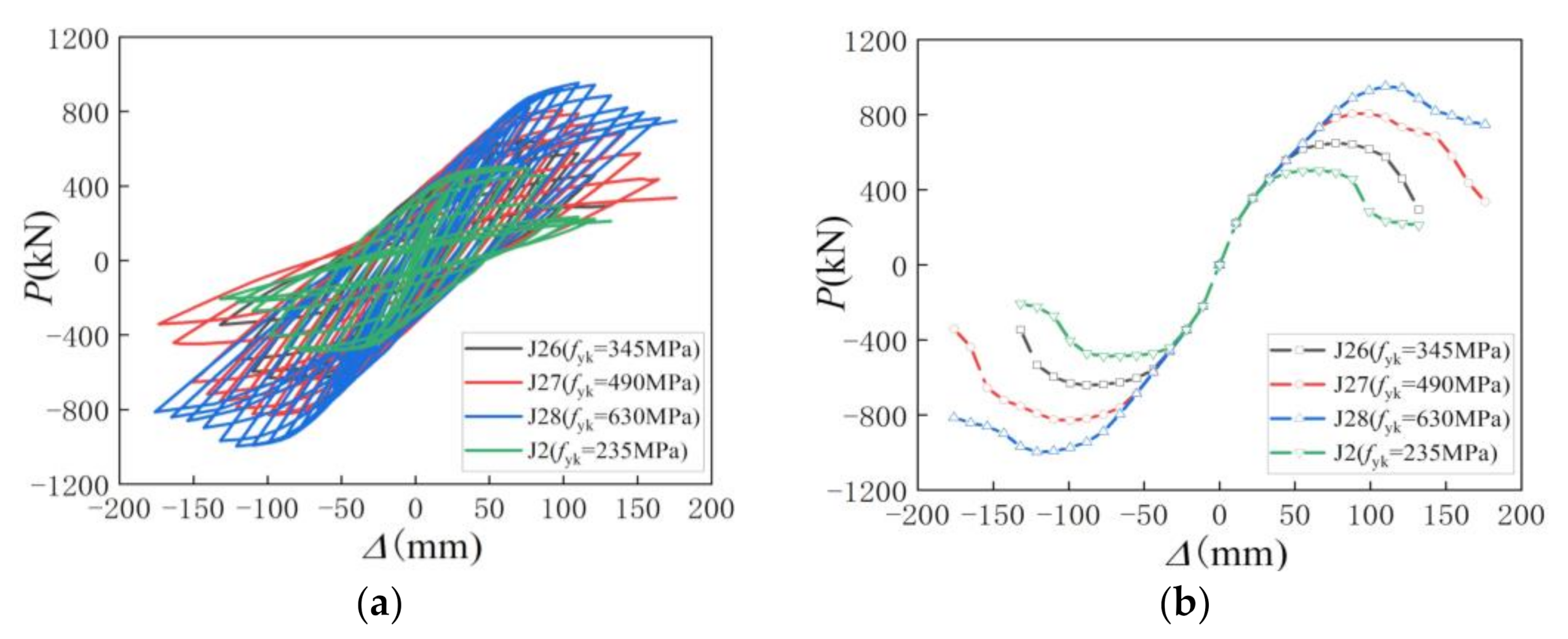
4.2.9. Yield Strengths of Steel Tubes (f_yk)

The hysteresis curves and P-Δ skeleton curves of specimens with different f_yk are shown in Figure 20. The load, displacement, and ductility coefficients of the specimens at each stage are shown in

Table 12. Load, displacement, and ductility coefficients of the specimens at each stage.

Specimen No.	fyk /mm	Pmax /kN	Δmax /mm	Py /kN	Δy /mm	Pu /kN	Δu /mm	μ
J2	235	503.38	60.74	438.71	31.60	402.04	91.24	2.89
J26	345	649.08	75.97	571.36	47.32	519.26	114.91	2.43
J27	490	808.17	89.77	731.18	67.10	646.54	147.74	2.20
J28	630	952.91	110.91	882.85	89.06	762.33	159.44	1.79

. It can be seen from Figure 20 and Table 12 that with the increasing of f_yk, P_max increases significantly. When f_yk increases from 235 to 345 MPa, 490 MPa, and 630 MPa, in turn, P_max of specimens increase from 503.38 to 649.08 kN, 808.17 kN, and 952.91 kN, which increases by 28.94%, 60.55%, and 89.3%, respectively. It can be seen that with the increasing of yield strengths of steel tubes, the P_max of the specimens increases significantly. When f_yk increases from 235 to 345 MPa, 490 MPa, and 630 MPa in turn, the μ of specimens decreases from 2.89 to 2.43, 2.20, and 1.79, which decreases by 15.92%, 23.88%, and 38.06%, respectively. It can be seen that with the increasing of f_yk, the ductility of the specimens becomes smaller, and the deformation capacity becomes worse. In practical engineering design, it is suggested that steel tubes with high strengths not be used.

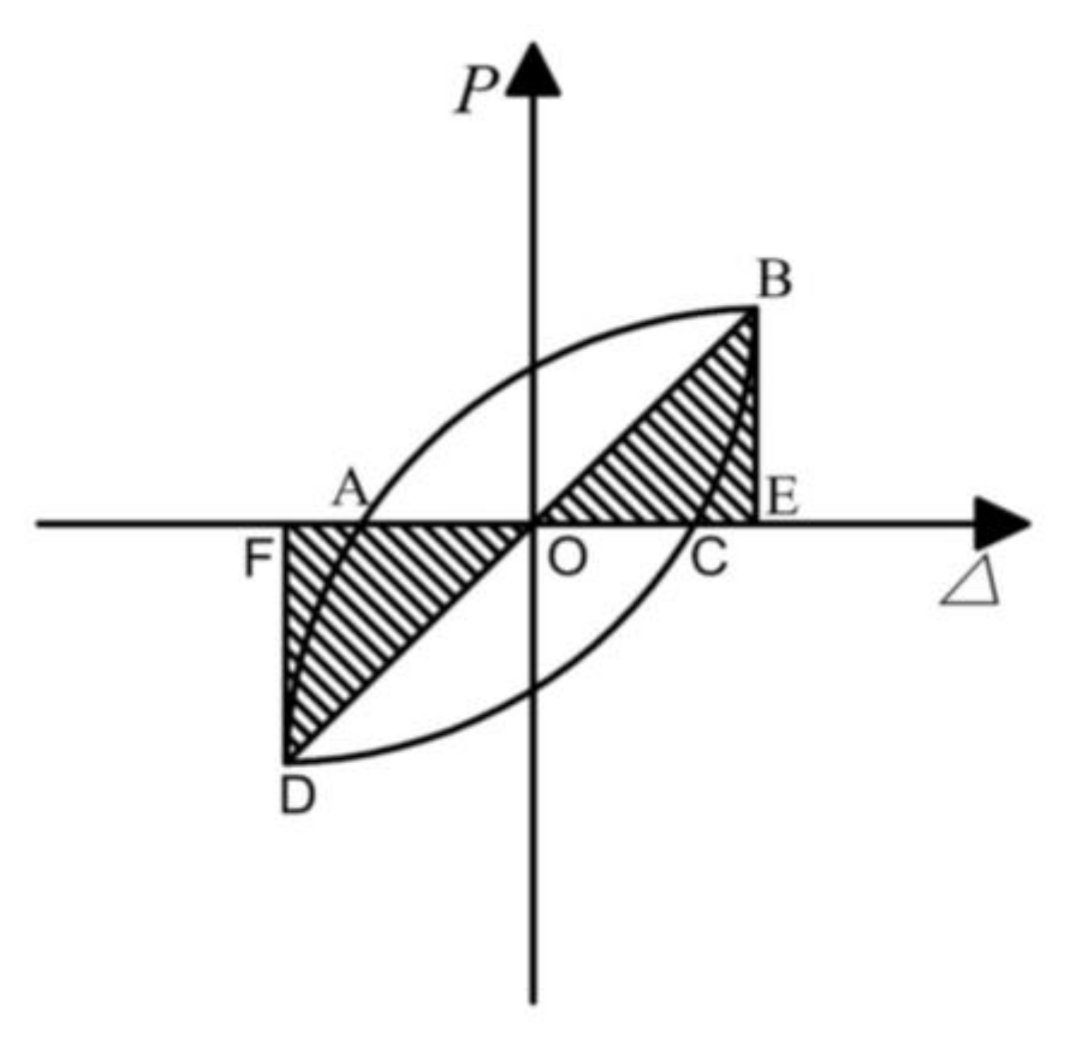
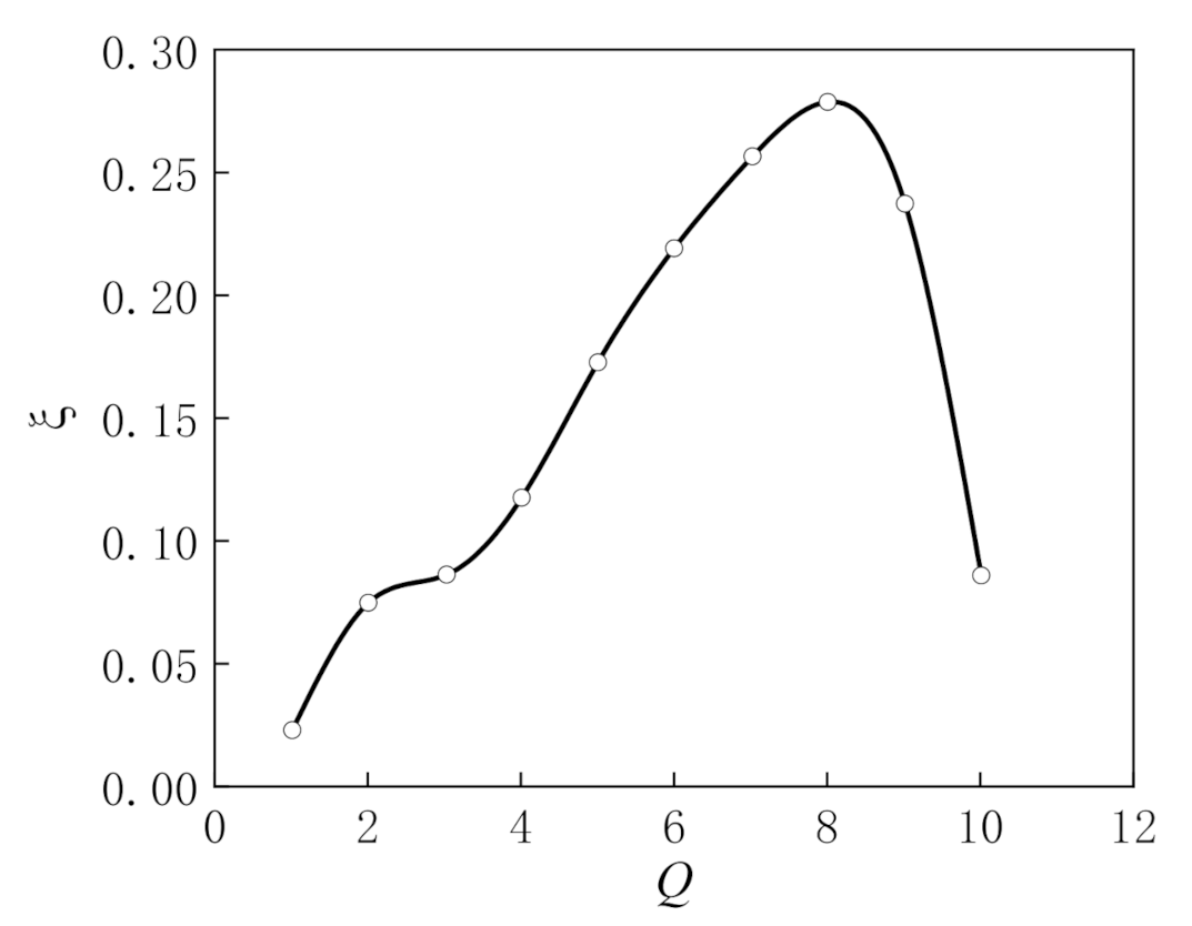
4.3. Energy Dissipation Capacity

Energy dissipation of structure is the energy expression of structural ductility. The more energy the structure absorbs and dissipates when it encounters an earthquake, the safer the structure will be, the fuller the hysteretic curves will be, and the larger the surrounding area will be. Energy dissipation coefficient E and equivalent viscous damping coefficient ξ are used to judge the energy dissipation capacity of the structure. The energy dissipation coefficient is calculated as shown in Figure 21, and the calculation formulas [29] are shown in Formulas (14) and (15); here, S represents the surrounding area. Energy dissipation coefficient (E) and equivalent viscous damping coefficient (ξ) corresponding to hysteretic loops of peak loading for 36 groups of specimens are shown in

Table 13. E and ξ of 36 specimens.

Specimen No.	h1 × b1 × t1 × t2 /mm4	h2× b2× t3× t4 /mm4	E (Peak Load)	ξ (Peak Load)
J1	840 × 300 × 10 × 14	540 × 300 × 10 × 14	1.755	0.279
J2	840 × 300 × 10 × 14	540 × 300 × 10 × 14	1.651	0.263
J3	840 × 300 × 10 × 14	540 × 300 × 10 × 14	1.681	0.268
J4	840 × 300 × 10 × 14	540 × 300 × 10 × 14	1.612	0.257
J5	840 × 300 × 10 × 14	540 × 300 × 10 × 14	1.685	0.268
J6	840 × 300 × 10 × 14	540 × 300 × 10 × 14	1.627	0.259
J7	840 × 300 × 10 × 14	540 × 300 × 10 × 14	1.623	0.258
J8	840 × 300 × 10 × 14	540 × 300 × 10 × 14	1.607	0.256
J9	840 × 300 × 10 × 14	540 × 300 × 10 × 14	1.604	0.255
J10	840 × 300 × 10 × 14	540 × 300 × 10 × 14	1.607	0.256
J11	840 × 300 × 10 × 14	540 × 300 × 10 × 14	1.682	0.268
J12	840 × 300 × 10 × 14	540 × 300 × 10 × 14	1.647	0.262
J13	840 × 300 × 10 × 14	540 × 300 × 10 × 14	1.641	0.261
J14	840 × 300 × 10 × 14	540 × 300 × 10 × 14	1.737	0.277
J15	840 × 300 × 10 × 14	540 × 300 × 10 × 14	1.569	0.250
J16	840 × 300 × 10 × 14	540 × 300 × 10 × 14	1.483	0.236
J17	840 × 300 × 10 × 14	540 × 300 × 10 × 14	1.574	0.251
J18	840 × 300 × 10 × 14	540 × 300 × 10 × 14	1.719	0.274
J19	800 × 300 × 10 × 14	540 × 300 × 10 × 14	1.659	0.264
J20	760 × 300 × 10 × 14	540 × 300 × 10 × 14	1.631	0.260
J21	720 × 300 × 10 × 14	540 × 300 × 10 × 14	1.689	0.269
J22	680 × 300 × 10 × 14	540 × 300 × 10 × 14	1.538	0.245
J23	840 × 300 × 10 × 14	460 × 300 × 10 × 14	1.640	0.261
J24	840 × 300 × 10 × 14	420 × 300 × 10 × 14	1.644	0.262
J25	840 × 300 × 10 × 14	380 × 300 × 10 × 14	1.638	0.261
J26	840 × 300 × 10 × 14	540 × 300 × 10 × 14	1.400	0.223
J27	840 × 300 × 10 × 14	540 × 300 × 10 × 14	1.134	0.181
J28	840 × 300 × 10 × 14	540 × 300 × 10 × 14	1.018	0.162
J29	840 × 300 × 10 × 14	540 × 300 × 8 × 14	1.664	0.265
J30	840 × 300 × 10 × 14	540 × 300 × 12 × 14	1.635	0.260
J31	840 × 300 × 10 × 14	540 × 300 × 14 × 14	1.630	0.260
J32	840 × 300 × 10 × 14	540 × 300 × 16 × 14	1.632	0.260
J33	840 × 300 × 10 × 14	540 × 300 × 10 × 10	1.630	0.260
J34	840 × 300 × 10 × 14	540 × 300 × 10 × 12	1.715	0.273
J35	840 × 300 × 10 × 14	540 × 300 × 10 × 16	1.743	0.278
J36	840 × 300 × 10 × 14	540 × 300 × 10 × 18	1.765	0.281

. Taking specimen J1 as an example, the ξ of each hysteretic loop (Q) is shown in Figure 22.

$$E=\frac{S_{ABC}+S_{CDA}}{S_{OBE}+S_{ODF}}$$

(14)

$$\xi =\frac{1}{2\pi }\frac{S_{ABC}+S_{CDA}}{S_{OBE}+S_{ODF}}$$

(15)

It can be seen from Table 13 that ξ of the composite joints under peak load is between 0.2 and 0.3. Previous studies have shown that the ξ of reinforced concrete joints under peak load is 0.1, while that of steel-reinforced concrete joints is about 0.3 [30]. Therefore, the ξ of all specimens is between ξ of reinforced concrete joints and ξ of steel-reinforced concrete joints. It can be seen that this kind of new asymmetrical composite joints have better energy dissipation capacity.

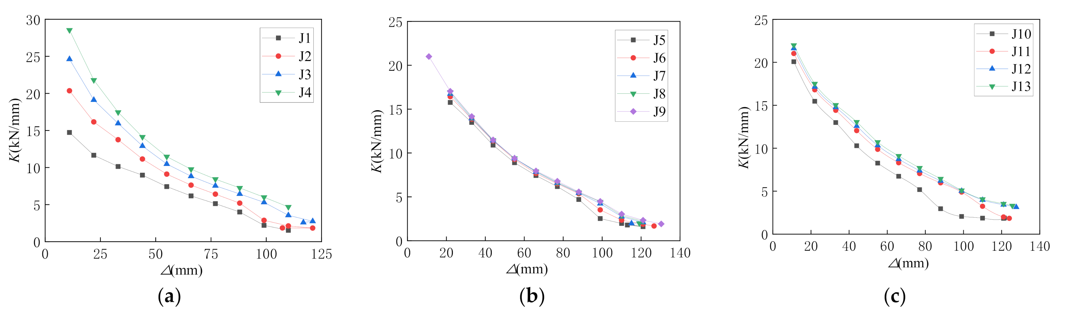
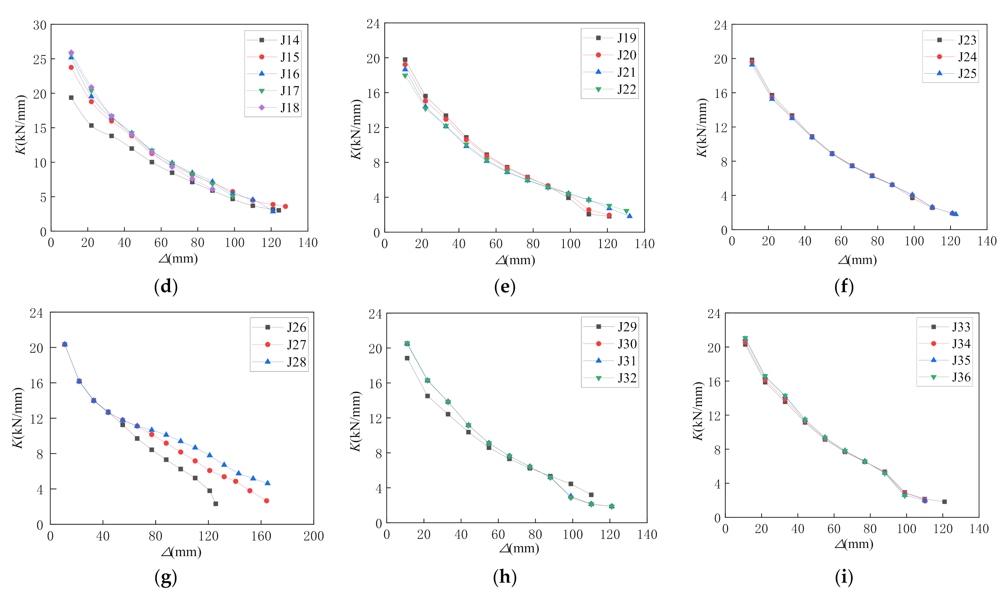
4.4. Stiffness Degradation

The stiffness of the specimens can be expressed by the secant stiffness (K) [31], which is defined as:

$$K=\frac{\left|+P_i\right|+\left|-P_i\right|}{\left|+{\Delta }_i\right|+\left|-{\Delta }_i\right|}$$

(16)

where $\pm P_i$ is the positive and negative peak load of each hysteresis loop, and $\pm {\Delta }_i$ is the positive and negative displacement corresponding to peak load. The influence of various parameters on K of specimens is shown in Figure 23. It can be seen from Figure 24 that with the increasing of displacement, the K value of all specimens gradually decreases, which shows the characteristics of stiffness degradation. It can be seen from Figure 23a that with the increasing of cross-sectional sizes of square steel tubes, K and the energy dissipation of the specimens gradually increases. It can be seen from Figure 23b that the compressive strength of cubic concrete has no obvious influence on K of the specimens. It can be seen from Figure 23c that with the increasing of wall thicknesses of the square steel tubes, K of the specimens gradually increases, but the increasing rate decreases. It can be seen from Figure 23d that with the increasing of axial compression ratio, K of specimens increases significantly, and the stiffness degrades significantly. It can be seen from Figure 23e,f that the heights of the high beams and the low beams have basically no effect on the K of specimens. It can be seen from Figure 23g that with the increasing of yield strengths of the steel tubes, K of the specimens is basically the same at the early stage. At the later stage, the steel tube enters the yielding stage, and K of the specimens increases significantly. It can be seen from Figure 23h that the web thickness and the flange thickness of the low beams have basically no effect on K of the specimens.

5. Shear Bearing Capacity

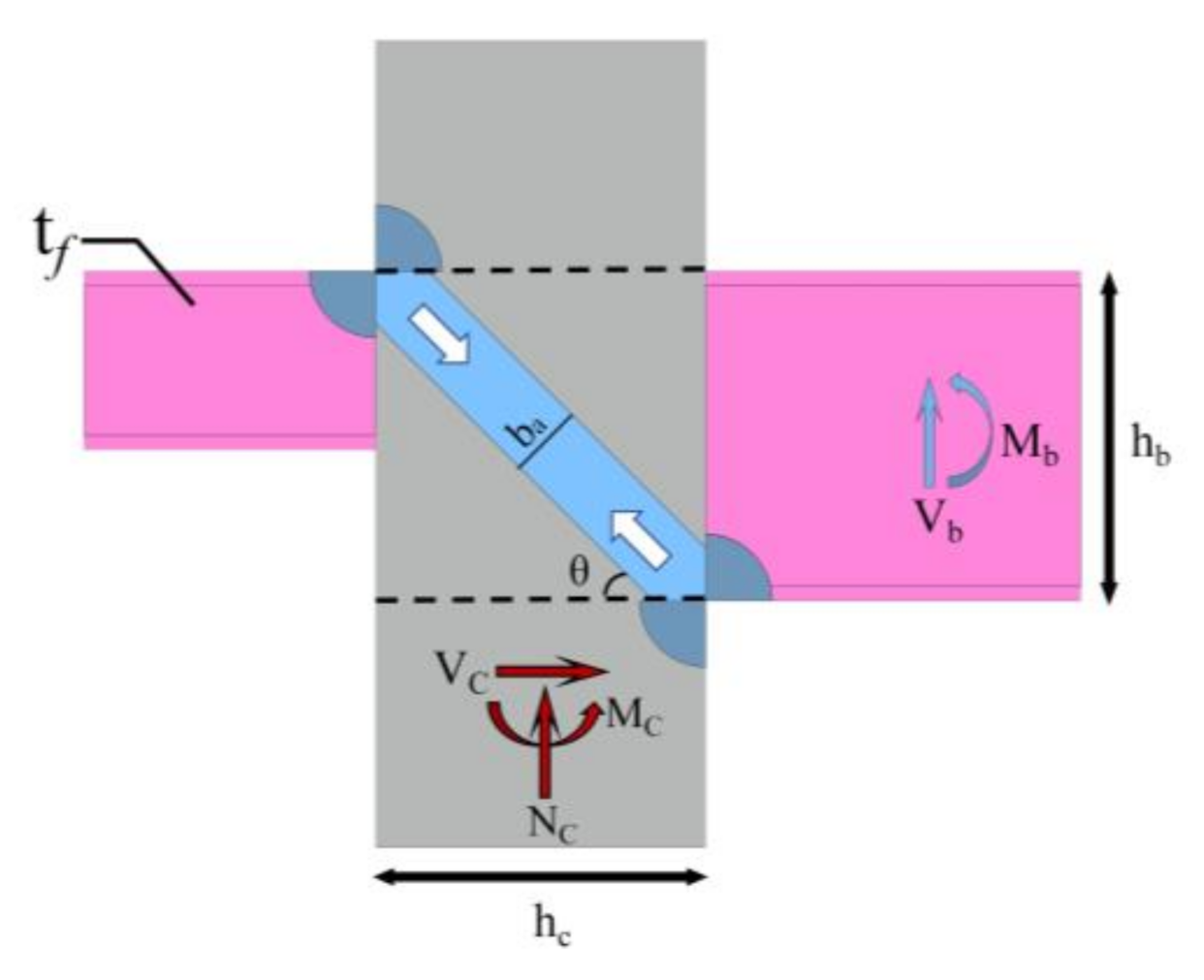
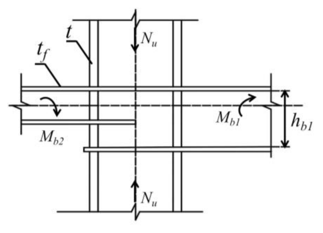
5.1. Stress Mechanism of Joints

At present, the shear failure mechanism of concrete at beam–column joints includes four mechanisms: diagonal strut mechanism, truss mechanism, shear friction mechanism, and constraint mechanism [32]. A diagonal strut mechanism is suitable for the joint applied by the vertical force and horizontal force. Oblique principal stress can be formed in the concrete of the joint domain. With the change of horizontal directions, oblique principal stress alternates positively and negatively, and a diagonal strut organization of concrete is formed [33]. The joints fail under compression, and the concrete in the core area of the joints achieves ultimate shear capacity, as shown in Figure 24. Due to the differences of heights between the left sides and right sides of the beams, shear yield firstly occurs in the upper core region and a baroclinic zone is formed in the core region of the joint at the initial loading stage. Under the constraint effect of steel tubes, the baroclinic zone becomes a baroclinic bar to bear shear loading. With the increasing of shear load, the whole yield area increases. At this time, the core concrete has not been completely crushed, and the bearing capacity can continue to increase. When reaching the limit state, the concrete in the core zone crushes, and the joint fails.

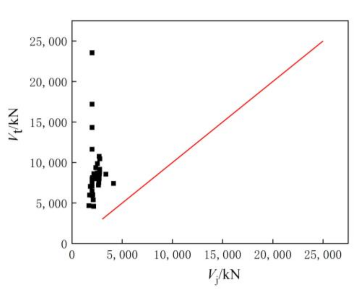
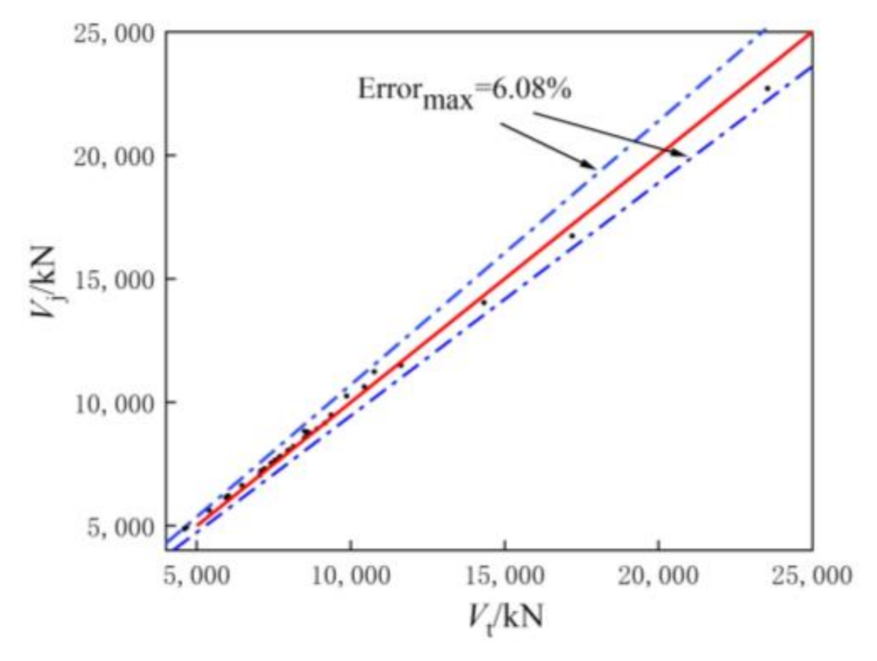
5.2. Shear Capacity of Joint Domain

Xu [17] believes that the diagonal strut in the core area of the joints is composed of the main diagonal strut and the constrained diagonal strut, and the sum of the shear capacity of these two bars in the horizontal direction is the shear capacity for the core area of joints. Based on this theory, the equation is established by using the virtual work principle, and the calculation shown in Formula (17) for the shear capacity of the asymmetrical composite joints with CFST columns and unequal height steel beams is obtained. The physical significance of each variable is shown in the literature [17]. The calculated value ($V_j$) by Equation (17) of the shear bearing capacity of 36 specimens is compared with the simulated value ($V_t)$, as shown in Figure 25.

$$V_j=\frac{1.8t\left(b-2t\right)\sqrt{f_{sy}^2-{\sigma }_s^2}}{\sqrt{3}}+\xi {\eta }_y{f}_c{b}_c\left(h_c-D\mathit{tan}\alpha \right)\mathit{cos}\alpha \mathit{sin}\alpha +2\mathit{sin}\alpha \sqrt{b{t}^2{f}_{sy}\xi {\eta }_y{f}_c{h}_c}$$

(17)

It can be seen that there is a large error between $V_j$ and $V_t$, so it is not suitable for this formula to calculate the shear bearing capacity of composite joints. According to the mechanism of joints, the shear capacity of joints is mainly composed of steel tubes and diagonal strut of concrete. The calculated shear capacity of the joint domain can be expressed as follows:

$$V_j=V_s+V_c$$

(18)

where $V_s$ is the shear capacity of steel tubes in joint domain, and $V_c$ is the shear capacity of concrete in the joint domain.

5.2.1. Shear Capacity of Concrete in Joint Domain

The horizontal shear force is resisted by concrete through the diagonal strut structure. According to the force mechanism of the diagonal strut of concrete, the shear capacity of concrete is taken as the horizontal component of the ultimate strength of the diagonal strut. The formula for the shear capacity of concrete at joint domain can be derived by reference [32] as follows:

$$V_c=f_c{b}_a{b}_c\mathit{cos}{\theta }_a$$

(19)

where $f_c$ is the axial compressive strength of concrete; $b_a$ is equivalent width of the diagonal strut; $b_c$ is the cross-sectional width of the concrete; and ${\theta }_a$ is the angle of concrete diagonal strut.

The height of the column is used to represent $b_a$, and its calculation formula is as follows:

$$b_a={\alpha }_a·\sqrt{h_c^2+h_b^2}={\gamma }_a{h}_c$$

(20)

where ${\gamma }_a={\alpha }_a\sqrt{1+{\beta }_j^2}$, ${\alpha }_a$ is the ratio of $b_a$ to the diagonal length of the joint domain, and its value is taken as 0.3 [34]. ${\beta }_j$ is the ratio of the heights of beams to columns, namely ${\beta }_j=\frac{h_b}{h_c}$.

${\theta }_a$ can be calculated according to the following formula:

$$\mathit{cos}{\theta }_a=\frac{h_{c0}-{\alpha }_s^{\prime }}{\sqrt{{\left(h_{c0}-{\alpha }_s^{\prime }\right)}^2+{\left(h_b-t_f\right)}^2}}$$

(21)

where $h_{c0}$ is the effective heights of columns. ${\alpha }_s^{\prime }$ is the distance between the resultant point of compressive reinforcement and the compression edge. $h_b$ is the height of the beams. $t_f$ is the flange thickness of steel beams.

The formula for the shear strength of concrete in the joint domain can be obtained by combining the above expressions:

$$V_c=0.3·f_c\sqrt{1+{\beta }_j^2}{h}_c{b}_c\mathit{cos}\theta .$$

(22)

5.2.2. Shear Capacity of Steel Tubes in Joint Domain

The calculation formula for shear stress of symmetrical steel beam–column joints is given in Standard for the design of steel structure of China [35], namely: $M_{b1}+M_{b2}=\frac{4}{3}\times f_v\times V_p$, and $V_s=f_v·S$. For asymmetrical beam–column joints, it is necessary to introduce the shear capacity correction factor ($\phi$) [36]:

$$\left(M_{b1}+M_{b2}\right)·\phi =\frac{4}{3}\times f_v\times V_p$$

(23)

$$\phi =a^{0.78}{\left(\frac{D}{t}\right)}^{0.41}{\left(\frac{b_f}{t_f}\right)}^{-0.31}{\left(1-n\right)}^{0.5}$$

(24)

$$V_P=1.8\times h_{b1}\times h_{c1}\times t_w.$$

(25)

The formula for V_s is as follows:

$$V_s=\frac{(M_{b1}+M_{b2})·S·\phi }{2.4\times h_{b1}·h_{c1}·t_w}$$

(26)

where $M_{b1}$ and $M_{b2}$ are the bending moments at both ends of the joints. S is the cross-sectional area of the steel tubes. a is the ratio of the heights on two sides. D is the width of the steel tubes. t is the wall thickness of the steel tubes. $\frac{b_f}{t_f}$ is the ratio of width to thickness of the flange. n is the axial compression ratio. $h_{b1}$ is the height between centerlines of flanges of high beams. $h_{c1}$ is the heights of webs of low beams. $t_w$ is the thickness of webs in the joint domain. The force state of the steel tubes in the joint domain is shown in Figure 26.

Compared with equal-height steel beams, unequal-height steel beams are subjected to asymmetric shear under cyclic loading, which will result in changes of the shear capacity for steel tubes and concrete. In order to take changes into consideration, the influence coefficients of concrete (${\xi }_1$) and steel tubes (${\xi }_2$) are introduced into Formula (18), and the shear capacity formula for composite joint domain is obtained by combining Formulas (18), (22) and (26):

$$V_j={\xi }_1·\frac{(M_{b1}+M_{b2})·S·\phi }{2.4\times h_{b1}·h_{c1}·t_w}+0.3·{\xi }_2{f}_c\sqrt{1+{\beta }_j^2}{h}_c{b}_c\mathit{cos}\theta .$$

(27)

The Levenberg–Marquardt (LM) optimization algorithm based on 1stOpt software is used to fit the data of 36 specimens. After 17 iterations, ${\xi }_1$ and ${\xi }_2$ are taken as 0.941 and 1.132, respectively. Submitting it into Formula (27), the formula for calculating the shear bearing capacity of the composite joint domain with CFST columns and unequal high steel beams can be obtained as follows:

$$V_j=0.941·\frac{(M_{b1}+M_{b2})·S·\phi }{2.4 \times h_{b1}·h_{c1}·t_w}+0.3396·f_c\sqrt{1+{\beta }_j^2}{h}_c{b}_c\mathit{cos}\theta .$$

(28)

According to Formula (28), the shear bearing capacity of the joint domain of 36 specimens can be calculated, and $V_j$ is compared with $V_t$, as shown in

Table 14. Comparisons between $V_j$ and $V_t$ for 36 specimens.

Specimen No.	${\mathit{V}}_{\mathit{t}}$ /kN	${\mathit{V}}_{\mathit{j}}$ /kN	${\mathit{V}}_{\mathit{t}}/{\mathit{V}}_{\mathit{j}}$	$\frac{\left|{\mathit{V}}_{\mathit{t}}-{\mathit{V}}_{\mathit{j}}\right|}{{\mathit{V}}_{\mathit{t}}} \times 100\%$
J1	4669.98	4937.71	0.95	5.73
J2	7954.73	8035.40	0.99	1.01
J3	9365.43	9480.90	0.99	1.23
J4	10,446.63	10,627.83	0.98	1.73
J5	7045.66	7042.40	1.00	0.05
J6	8614.23	8793.55	0.98	2.08
J7	8502.30	8825.83	0.96	3.81
J8	9872.72	10,252.92	0.96	3.85
J9	10,766.66	11,231.68	0.96	4.32
J10	5979.56	6181.45	0.97	3.38
J11	7980.75	8055.29	0.99	0.93
J12	8696.14	8723.85	0.99	0.32
J13	9166.14	9161.51	1.00	0.05
J14	8903.58	8914.46	0.99	0.12
J15	8598.74	8627.62	0.99	0.34
J16	7998.45	8062.77	0.99	0.80
J17	7522.83	7615.24	0.98	1.23
J18	7199.33	7310.84	0.98	1.55
J19	8136.54	8206.47	0.99	0.86
J20	6020.75	6215.62	0.96	3.24
J21	5394.80	5626.63	0.95	4.30
J22	4592.46	4871.67	0.94	6.08
J23	14,328.78	14,033.06	1.02	2.06
J24	17,194.81	16,729.85	1.03	2.70
J25	23,547.71	22,707.60	1.04	3.57
J26	8499.26	8547.77	0.99	0.57
J27	8552.20	8597.59	0.99	0.53
J28	7417.76	7530.14	0.98	1.51
J29	11,634.10	11,497.49	1.01	1.17
J30	7083.73	7215.83	0.98	1.86
J31	6466.99	6635.51	0.97	2.61
J32	5947.72	6146.90	0.97	3.35
J33	7959.84	8040.21	0.99	1.01
J34	7685.80	7782.35	0.99	1.26
J35	7548.19	7652.87	0.99	1.39
J36	7714.58	7809.43	0.99	1.23

. The dispersion degree of $V_j$ and $V_t$ can be seen in Figure 27, and the maximum error (Error_max) is 6.08%. It can be seen that the formula has high calculation accuracy and can meet engineering needs [37,38].

6. Conclusions

The full-scale finite element models of 36 asymmetrical composite joints with CFST columns and unequal high steel beams were established reasonably. The influence regularity of different parameters on the hysteretic performance of the asymmetrical composite joints was clarified. The expression for the shear bearing capacity of asymmetrical full-scale composite joints is obtained. The specific conclusions are as follows:

(1) With the increasing of f_cuk, the peak load and ductility of the specimens gradually increase. With the increasing of the wall thickness of the square steel tubes and sectional sizes of square steel tubes, the peak load and ductility of the specimens can be significantly improved. It can be seen that the steel tube has a significant restraint effect on concrete. When the axial compression ratio is 0.4, the specimens have better bearing capacity and ductility. ξ of the composite joints under peak load is between 0.2 and 0.3, which shows that this new type of composite joints has better energy dissipation capacity. With the increasing of displacement, K of all specimens gradually decreases, which shows the characteristics of stiffness degradation.

(2) The shear capacity of this type of joints is mainly composed of the shear capacity of steel tubes and diagonal strut of concrete. Shear yielding firstly occurs in the upper core region and diagonal struts are formed in the core joint region at the initial loading stage. With the increasing of shear loading, the whole yield area increases. When reaching the limit state, the concrete in the core zone crushes, and the joint fails.

References

1. Pei, S.L.; Van de Lindt, J.W. Systematic seismic design for manageable loss in wood-framed buildings. Earthq. Spectra 2009, 25, 851–868. [Google Scholar] [CrossRef]
2. Van de Lindt, J.W.; Gupta, R.; Pei, S.L.; Tachibana, K. Damage assessment of a full-scale six-story wood-frame building following triaxial shake table tests. J. Perform. Constr. Facil. 2012, 26, 17–25. [Google Scholar] [CrossRef] [Green Version]
3. Zhou, W. Analysis on Seismic Performance of Reinforced Concrete Frame Structure including Vertical Ground Motion Based on Wenchuan Earthquake. Master’s Thesis, Lanzhou University of Technology, Lanzhou, China, 2011. [Google Scholar]
4. Wang, J. Seismic damage analysis of reinforced concrete frame structure and the importance of ductility design. Fujian Build. Mater. 2011, 1, 47–49. [Google Scholar]
5. Han, S.W.; Kim, T.O.; Baek, S.J. Seismic performance evaluation of steel ordinary moment frames. Earthq. Spectra 2018, 34, 55–76. [Google Scholar] [CrossRef]
6. Fan, J.S.; Li, Q.W.; Nie, J.G.; Zhou, H. Experimental study on the seismic performance of 3d joints between concrete-filled square steel tubular columns and composite beams. J. Struct. Eng. 2014, 140, 1–13. [Google Scholar] [CrossRef]
7. Li, B.; Leong, C.L. Experimental and Numerical Investigations of the Seismic Behavior of High-Strength Concrete Beam-Column Joints with Column Axial Load. J. Struct. Eng. 2015, 141, 1–14. [Google Scholar] [CrossRef]
8. Saeedeh, G.; Ali, K.; Meissam, N.; Masoud, M.S.; Majid, G. Nonlinear behavior of connections in RCS frames with bracing and steel plate shear wall. Steel Compos. Struct. 2016, 22, 915–935. [Google Scholar]
9. Jeddi, M.; Sulong, R.; Khanouki, A. Seismic performance of a new through rib stiffener beam connection to concrete-filled steel tubular columns: An experimental study. Eng. Struct. 2017, 131, 477–491. [Google Scholar] [CrossRef]
10. Ghomi, S.K.; Ehab, E.S. Effect of joint shear stress on seismic behavior of interior GFRP-RC beam-column joints. Eng. Struct. 2019, 191, 583–597. [Google Scholar] [CrossRef]
11. Bian, J.L.; Cao, W.L.; Zhang, Z.M.; Qiao, Q.Y. Cyclic loading tests of thin-walled square steel tube beam-column joint with different joint details. Structures 2020, 25, 386–397. [Google Scholar] [CrossRef]
12. Zheng, X.W. Study on the Mechanical Behaviors of Steel Frames Beam-to-Column T-Stub Connection Joint under Cyclic Load. Master’s Thesis, Guangxi University, Nanning, China, 2013. [Google Scholar]
13. Liu, J.X.; Dai, S.B.; Huo, K.C.; Huang, J.; Lin, M.S. Study on earthquake resistance behavior of top and seat angle joint of special-shaped concrete-filled rectangular composite tubular column with steel beam. J. Sichuan Univ. 2015, 47, 128–137. [Google Scholar]
14. Mou, B.; Jing, H.; Zhang, C.; Wang, Y.; Wang, Y. Experimental investigation on seismic behavior of unequal-depth H-shaped steel beam to square steel column connection with external-diaphragm. J. Build. Struct. 2018, 39, 80–89. [Google Scholar]
15. Xia, J.; Zhu, H.Q.; Zhang, Z.X.; Chang, H.F. Static performance of H-beam to square tubular column interior joint with splicing outer sleeve. J. Build. Struct. 2018, 39, 104–114. [Google Scholar]
16. Dai, Y.; Nie, S.F.; Zhou, T.H. Shear capacity of circular steel tube confined H-SRC concrete column steel beam joint with ring beam. J. Jilin Univ. 2021, 3, 977–988. [Google Scholar]
17. Xu, C.X.; Fei, J.B.; Jian, Q.A.; Peng, S. Analysis on shear capacity of frame joints with concrete-filled square steel tubular columns and unequal height steel beams. World Earthq. Eng. 2020, 36, 53–61. [Google Scholar]
18. Xu, C.X.; Gao, J.; Qiu, Y.W.; Xiao, L.L. Seismic Performance Analysis on Concrete-filled Square Steel Tubular Column-unequal Depth Steel Beam Frame Joints Based on OpenSees. Sci. Technol. Eng. 2019, 19, 276–283. [Google Scholar]
19. Xu, C.X.; Qiu, Y.W.; Jian, Q.A.; Lu, Y.F. Experimental study on seismic behavior of joints in the frame with concrete-filled steel square tubular column and H-shaped unequal height steel beam. Build. Struct. 2019, 49, 48–55. [Google Scholar]
20. Han, L.H.; Tao, Z.; Liu, W. Concrete filled steel tubular structures from theory to practice. J. Fuzhou Univ. 2001, 6, 24–34. [Google Scholar]
21. Teng, J.G.; Yu, T.; Wong, Y.L.; Dong, S.L. Hybrid FRP-concrete-steel tubular columns: Concept and behavior. Constr. Build. Mater. 2007, 21, 846–854. [Google Scholar] [CrossRef]
22. Pagoulatou, M.; Sheehan, T.; Dai, X.H.; Lam, D. Finite element analysis on the capacity of circular concrete-filled double-skin steel tubular (CFDST) stub columns. Eng. Struct. 2014, 72, 102–112. [Google Scholar] [CrossRef] [Green Version]
23. Housing and Urban-Rural Development of the People’s Republic of China. Code for Design of Concrete Structures: GB50010-2010; China Architecture & Building Press: Beijing, China, 2010.
24. Zhang, S.; Cheng, M.; Wang, J.; Wu, J.Y. Modeling the hysteretic responses of RC shear walls under cyclic loading by an energy-based plastic-damage model for concrete. Int. J. Damage Mech. 2020, 29, 184–200. [Google Scholar] [CrossRef]
25. Li, Z.H.; Gu, H.C. Bauschinger effect and residual phase stresses in two ductile-phase steels: Part I. The influence of phase stresses on the Bauschinger effect. Metall. Trans. A 1990, 21, 717–724. [Google Scholar]
26. Ji, J.; Zhang, R.B.; Yu, C.Y.; He, L.J.; Ren, H.G.; Jiang, L.Q. Flexural Behavior of Simply Supported Beams Consisting of Gradient Concrete and GFRP Bars. Front. Mater. 2021, 8, 1–14. [Google Scholar] [CrossRef]
27. Ji, J.; Zeng, W.; Wang, R.L.; Ren, H.G.; Zhang, L. Bearing Capacity of Hollow GFRP Pipe-Concrete-High Strength Steel Tube Composite Long Columns under Eccentrical Compression Load. Front. Mater. 2021, 8, 1–15. [Google Scholar] [CrossRef]
28. Park, R. Evaluation of Ductility of Structures and Structural Assemblages from laboratory Testing. Bull. N. Z. Natl. Soc. Earthq. Eng. 1989, 22, 155–166. [Google Scholar] [CrossRef]
29. Ji, J.; Xu, Z.C.; Jiang, L.Q.; Yuan, C.Q. Nonlinear Buckling Analysis of H-Type Honeycombed Composite Column with Rectangular Concrete-Filled Steel Tube Flanges. Int. J. Steel Struct. 2018, 18, 1153–1166. [Google Scholar] [CrossRef]
30. Jiang, J.J. Nonlinear Finite Element Analysis of Reinforced Concrete Structure; Shaanxi Science and Technology Press: Xi’an, China, 1994. [Google Scholar]
31. Zheng, W.Z.; Ji, J. Dynamic performance of angle-steel concrete columns under low cyclic loading-I: Experimental study. Earthq. Eng. Eng. Vib. 2008, 7, 67–75. [Google Scholar] [CrossRef]
32. Zhang, S.H.; Zhang, X.Z.; Zhang, T.H.; Li, X.Q.; Ding, Y.J.; Jia, L. Experimental study on seismic behavior of concrete-filled precast concrete tube column to steel beam connections. J. Build. Struct. 2020, 41, 1–13. [Google Scholar]
33. Cai, Z.W.; Liu, F.C.; Yu, J.T.; Yu, K.Q.; Tian, L.K. Development of ultra-high ductility engineered cementitious composites as a novel and resilient fireproof coating. Constr. Build. Mater. 2021, 288, 123090. [Google Scholar] [CrossRef]
34. Tang, J.R. Seismic Resistance of Joints in Reinforced Concrete Frames; Southeast University Press: Nanjing, China, 1989. [Google Scholar]
35. Housing and Urban-Rural Development of the People’s Republic of China. Standard for Design of Steel Structure: GB50017-2017; China Architecture & Building Press: Beijing, China, 2018.
36. Zheng, Z.X. 2D and 3D Irregular Steel Partial Frame Research on the Elastic-Plastic Characteristic. Master’s Thesis, Shenyang Jianzhu University, Shenyang, China, 2015. [Google Scholar]
37. Ji, J.; Yang, M.M.; Xu, Z.C.; Jiang, L.Q.; Song, H.Y. Experimental Study of H-Shaped Honeycombed Stub Columns with Rectangular Concrete-Filled Steel Tube Flanges Subjected to Axial Load. Adv. Civ. Eng. 2021, 2021, 6678623. [Google Scholar] [CrossRef]
38. Mushtaq, A.; Ali Khan, S.; Farooq Gabriel, H.; Haider, S. Seismic vulnerability assessment of deficient RC structures with bar pullout and joint shear degradation. Adv. Civ. Eng. 2015, 2015, 537405. [Google Scholar] [CrossRef]
Figure 1. Constitutive models of concrete.
Symmetry 13 02381 g001
Figure 2. Constitutive model of steel.
Symmetry 13 02381 g002
Figure 3. Three-dimensional geometric model.
Symmetry 13 02381 g003
Figure 4. Detailed diagram of MPC constraints: (a) low beam; (b) bottom of column; (c) high beam.
Symmetry 13 02381 g004
Figure 5. Comparisons of skeleton curves of specimens with different meshing sizes: (a) specimen CFSTJ-1; (b) specimen CFSTJ-2.
Symmetry 13 02381 g005
Figure 6. Mesh division of the specimens with partial densification.
Symmetry 13 02381 g006
Figure 7. Comparisons of hysteresis curves between simulations and tests: (a) specimen CFSTJ-1; (b) specimen CFSTJ-2; (c) specimen CFSTJ-3; (d) specimen CFSTJ-4.
Symmetry 13 02381 g007aSymmetry 13 02381 g007b
Figure 8. Comparisons of skeleton curves between simulations and tests: (a) specimen CFSTJ-1; (b) specimen CFSTJ-2; (c) specimen CFSTJ-3; (d) specimen CFSTJ-4.
Symmetry 13 02381 g008
Figure 9. Stress cloud diagram of models and failure modes of tests: (a) specimen CFSTJ-1; (b) specimen CFSTJ-2.
Symmetry 13 02381 g009
Figure 10. The specific size of specimen J1: (a) dimensions of beams and columns (mm); (b) connecting plate size (mm); (c) beam section size (mm).
Symmetry 13 02381 g010
Figure 11. Comparisons of curves of joints with different strengths of concrete: (a) hysteretic curves; (b) skeleton curves.
Symmetry 13 02381 g011
Figure 12. The yield point is determined by Park method.
Symmetry 13 02381 g012
Figure 13. Comparisons of curves of joints with different axial pressure ratios: (a) hysteretic curves; (b) skeleton curves.
Symmetry 13 02381 g013
Figure 14. Comparisons of curves of joints with different heights of low beams: (a) hysteretic curves; (b) skeleton curves.
Symmetry 13 02381 g014
Figure 15. Comparisons of curves of joints with different wall thicknesses of square steel tubes: (a) hysteretic curves; (b) skeleton curves.
Symmetry 13 02381 g015
Figure 16. Comparisons of curves for joints with different flange thicknesses of low beams: (a) hysteretic curves; (b) skeleton curves.
Symmetry 13 02381 g016
Figure 17. Comparisons of curves for joints with different web thicknesses of low beams: (a) hysteretic curves; (b) skeleton curves.
Symmetry 13 02381 g017
Figure 18. Comparisons of curves for joints with different heights of the high beams: (a) hysteretic curves; (b) skeleton curves.
Symmetry 13 02381 g018
Figure 19. Comparisons of curves for joints with different cross-sectional dimensions: (a) hysteretic curves; (b) skeleton curves.
Symmetry 13 02381 g019
Figure 20. Comparisons of curves for joints with different yield strengths of steel tubes: (a) hysteretic curves; (b) skeleton curves.
Symmetry 13 02381 g020
Figure 21. Schematic diagram for calculating E.
Symmetry 13 02381 g021
Figure 22. ξ of each loop of J1 joint.
Symmetry 13 02381 g022
Figure 23. Comparisons of stiffness degradation curves of each group of specimens: (a) different cross-sectional sizes of the square steel tubes; (b) different compressive strengths of cube concrete; (c) different wall thicknesses of the square steel tubes; (d) different axial compression ratios; (e) different heights of the high beams; (f) different heights of the low beams; (g) different yield strengths of steel tubes; (h) different web thicknesses of the low beams; (i) different flange thicknesses of the low beams.
Symmetry 13 02381 g023aSymmetry 13 02381 g023b
Figure 24. The stress mechanism of concrete in the joint domain.
Symmetry 13 02381 g024
Figure 25. Comparisons of shear capacity for 36 specimens.
Symmetry 13 02381 g025
Figure 26. The force state of the steel tubes in the joint domain.
Symmetry 13 02381 g026
Figure 27. Comparisons between V t and V j for 36 specimens.
Symmetry 13 02381 g027