Asymmetric Design Sensitivity and Isogeometric Shape Optimization Subject to Deformation-Dependent Loads

Abstract

We present a design sensitivity analysis and isogeometric shape optimization with path-dependent loads belonging to non-conservative loads under the assumption of elastic bodies. Path-dependent loads are sometimes expressed as the follower forces, and these loads have characteristics that depend not only on the design area of the structure but also on the deformation. When such a deformation-dependent load is considered, an asymmetric load stiffness matrix (tangential operator) in the response region appears. In this paper, the load stiffness matrix is derived by linearizing the non-linear non-conservative load, and the geometrical non-linear structure is optimally designed in the total Lagrangian formulation using the isogeometric framework. In particular, since the deformation-dependent load changes according to the change and displacement of the design area, the isogeometric analysis has a significant influence on the accuracy of the sensitivity analysis and optimization results. Through several numerical examples, the applicability and superiority of the isogeometric analysis method were verified in optimizing the shape of the problem subject to deformation-dependent loads.

1. Introduction

Special attention is required in the structural analysis of the pressure loading, as its loading direction could change with the deformation of the structure. Engineering problems with deformation-dependent loading are frequently encountered, for example, in the design of dams, tires, airbags, and pressurized vessels. When such a deformation-dependent load is considered, an asymmetric tangential operator expressed as a load stiffness matrix appears in the governing equation. Hibbit [1] first mentioned the concept of load stiffness, and in the case of a surface traction load, the load stiffness is symmetric if it is applied to the fully enclosed volume. If it is not the case, the equation has an asymmetric term which is to be solved using the approximation method, assuming it is symmetric while refining the mesh.

In the previous study from Mok et al. [2], the pressure load was decomposed to the body-attached pressure load and the space-attached pressure load. They derived the load stiffness term by linearizing the nonlinear pressure load term. Simo [3] expressed the pressure-loaded moving boundary in an isoparametric presentation and obtained the tangent stiffness through linearization of the loading boundary. In addition, the convergence rate dependent on tangent stiffness was discussed in numerical examples for an axisymmetric case.

If the pressure loading is considered in the design optimization, it becomes a function of both the deformation by loading and the design change on boundaries. Many previous studies have been conducted for the pressure loading in the design boundaries. Kim et al. [4] optimized the structure of sheet metal subjected to a pressure load. They performed a design sensitivity analysis by taking variations in the parametric domain with the employment of the parametric representation method for the pressure load. They presented the effect of the deformation-dependent loads on the optimization performance. In their shape sensitivity analysis on the design-dependent loadings, Akbari et al. [5] demonstrated the equivalence between continuum and discrete derivatives. Hammer and Olhoff [6] presented the generalization of topology optimization of linear elastic structures for the problems which involve design-dependent loading. Kiendl et al. [7] studied an isogeometric optimization for the tube subject to the internal pressure using semi-analytical sensitivity analysis and sensitivity weighting. Picelli et al. [8] investigated topology optimization for design-dependent hydrostatic pressure loading via the level-set method.

To consider the deformation and design change in the boundaries correctly, an accurate geometric representation is essential. The isogeometric analysis (IGA) first proposed by Hughes et al. [9] enables the exact parametrization of loading and design boundaries by employing the NURBS basis function that is now the standard tool in the computer-aided design (CAD) industry. First of all, the properties of the NURBS basis function enable a more accurate geometric representation than the traditional finite element or meshfree method. The NURBS basis function and the resultant geometric representation allow for an accurate representation of the analysis model even when using the coarse mesh. In the formulation of general elasticity problems, as opposed to the finite element method which approximates the model in a partially linearized way, IGA expresses the geometric information of the shape with NURBS basis functions and provides the continuous characteristic in the variational formulation. Therefore, it is natural to adopt the isogeometric framework in the shape optimization [10,11] for the case of a deformation-dependent load.

As opposed to conservative dead loading, follower loading maintains its orientation to the structure as it deforms. Consider a pressure load that is dependent on the deformation as shown in Figure 1.

The fixed load, p⁰, in Figure 1a is a distributed load defined at initial configuration without any changes, and the design-dependent load, p(d), in Figure 1b is the pressure load with the changed loading direction according to perturbed design (d). The symmetric shape sensitivity analysis for the design-dependent load in Figure 1b with the assumption of infinitesimal strain was previously derived and utilized in several optimization problems in the isogeometric framework [12,13].

On the other hand, the design- and deformation-dependent load, p(d, u), in Figure 1c changes according to the deformation (u) and the variation of design (d), which leads to an asymmetric load stiffness matrix by linearization in the response and design sensitivity analysis. In this paper, the isogeometric continuum-based sensitivity analysis suggested by Cho and Ha [14] is performed for accurate sensitivity analysis of the problems subject to a design- and deformation-dependent load. The design boundary change expressed by the NURBS basis function leads to a natural shape change, which leads to accurate design shape sensitivity. The design sensitivity analysis based on the geometric analysis method was induced by the design sensitivity theory [15,16], and its accuracy is verified for the response field. The asymmetric sensitivity equation for the deformation-dependent loadings is expressed as the dependent term according to the displacement and the design change of the structure in Figure 1c, including the geometric higher-order terms such as normal vector and curvature. Compared to the traditional finite element-based sensitivity analysis, NURBS-based design sensitivity analysis results in accurate sensitivity values because the load-stiffness matrix by the deformation- and design-dependent loads, in general taking an asymmetric form, is incorporated into the sensitivity equation.

The remainder of this paper is organized as follows. Section 2 of this paper briefly explains the B-spline basis function and provides a brief explanation of the features of the geometric analysis based on it. We formulate a load representation that describes the characteristics of a pressure load in a continuum form and develop a governing equation and a weak formulation for a geometric nonlinear structure in a Lagrangian formulation, which incorporates the asymmetric load stiffness terms. The details on our formulation of the design sensitivity equations for geometric nonlinear structures subjected to deformation-dependent pressure loads are also described. In Section 3, numerical examples showing the accuracy of isogeometric continuum-based sensitivity compared based on the isogeometric approach to that of finite difference for the structures subjected to deformation-dependent loads are presented. Through the shape optimization examples, the efficiency and applicability of the proposed method will also be checked. Finally, in Section 4, we summarize the conclusions, explaining the importance of the isogeometric analysis method in nonlinear structures subjected to pressure loads.

2. Materials and Methods

2.1. Overview of NURBS Basis Function and Isogeometric Analysis

In isogeometric analysis (IGA), the solution space adopts the same NURBS basis function to describe the geometry. Over the conventional finite element method, IGA has several advantages: exact geometry representation and simple refinement process non-interacting with CAD system due to the use of NURBS basis functions based on B-splines [9]. With the set of knots ${\xi }_i$ in parametric space, a knot vector $\Xi$ is defined in a one-dimensional space,

$$\Xi =\left\{{\xi }_1,{\xi }_2,\cdots ,{\xi }_{n+p+1}\right\}$$

(1)

where p is the order of the basis function, and n is the number of control points. The B-spline basis functions are defined, recursively, as

$$N_{i,0}\left(\xi \right)=\left\{\begin{array}{ll}1& \mathrm{if} {\xi }_i\le \xi <{\xi }_{i+1}\\ 0& \mathrm{otherwise} \end{array}\right.,\hspace{0.33em}\left(p=0\right)$$

(2)

and

$$N_{i,p}\left(\xi \right)=\frac{\xi -{\xi }_i}{{\xi }_{i+p}-{\xi }_i}{N}_{i,p-1}\left(\xi \right)+\frac{{\xi }_{i+p+1}-\xi }{{\xi }_{i+p-1}-{\xi }_{i+1}}{N}_{i+1,p-1}\left(\xi \right),\hspace{0.33em}\left(p=1,2,3,\dots \right)$$

(3)

Using the B-spline basis function $N_{i,p}\left(\xi \right)$ and weight $w_i$, the NURBS basis function $R_{i,p}\left(\xi \right)$ is defined as

$$R_{i,p}\left(\xi \right)=\frac{N_{i,p}\left(\xi \right)w_i}{{\displaystyle \sum _{j=1}^n{N}_{j,p}\left(\xi \right)w_j}}$$

(4)

In general, the higher-order basis functions in IGA offer higher regularity than the conventional finite element approach. The NURBS possesses the following desirable properties as a basis function.

For the given $n$ pairs of the p-th order NURBS basis function $R_{i,p}\left(\xi \right)$ and the corresponding projected weighted control point $B_i\equiv B\left(x_i\right)$, a NURBS curve C is obtained by

$$C\left(\xi \right)={\displaystyle \sum _{i=1}^n{R}_{i,p}\left(\xi \right)B_i}$$

(5)

In the same manner, NURBS surface is defined as a product of NURBS basis functions,

$$S\left(\Xi \right)\equiv S\left(\xi ,\eta \right)={\displaystyle \sum _{i=1}^l{\displaystyle \sum _{j=1}^m{R}_{i,p}^{}\left(\xi \right)R_{j,q}^{}\left(\eta \right)}} B_{i,j}\equiv {\displaystyle \sum W_I^p\left(\Xi \right)}{B}_I$$

(6)

In isogeometric analysis, geometric points and responses are expressed using the relation (6):

$$x\left(\Xi \right)={\displaystyle \sum W_I^p\left(\Xi \right)}{B}_I\left(x\right)$$

(7)

and

$$z\left(\Xi \right)={\displaystyle \sum W_I^p\left(\Xi \right)}\hspace{0.33em}{u}_I$$

(8)

where $B_I\left(x\right)=B\left(x_1,x_2,x_3\right)$ are the control points, and $u_I=u\left(x_1,x_2,x_3\right)$ are called the response coefficients at the control points. Note that the NURBS basis functions have a non-interpolatory property.

2.2. Isogeometric Shape Sensitivity Analysis for Pressure Load

2.2.1. Isogeometric Analysis of Geometrically Nonlinear Structure for Following Load Problem

The equilibrium of a deformable body at current configuration (n + 1) under deformation- and design-dependent load can be expressed by using the principle of virtual work in total Lagrangian formulation as

$$a\left({}^{n+1}z,\overline{z}\right)=\ell \left({}^{n+1}z,\overline{z}\right)$$

(9)

where the strain energy and load form are defined, respectively, as

$$a\left({}^{n+1}z,\overline{z}\right)\equiv {\displaystyle {\int }_{{}^0\mathsf{\Omega }}{c}_{ijkl}{\epsilon }_{kl}({}^{n+1}z){\stackrel{⌢}{\epsilon }}_{ij}\left({}^{n+1}z;\overline{z}\right)d{}^0\mathsf{\Omega }}$$

(10)

and

$$\ell \left({}^{n+1}z,\overline{z}\right)\equiv -{\displaystyle {\int }_{{}^0\mathsf{\Gamma }}^{}{\overline{z}}_i}p{F}_{ji}^{-1}\left({}^{n+1}z\right)N_{j}J\left({}^{n+1}z\right)d{}^0\mathsf{\Gamma },$$

(11)

and $c_{ijkl}$, $z$, $\overline{z}$ and $\overline{Z}$ are material response tensor, displacement, virtual displacement, and variational space, respectively.

Generally, the pressure boundary at the current configuration (n + 1) can be represented as shown in Figure 2:

$$nd{}^{n+1}\mathsf{\Gamma }=F{\left({}^{n+1}z\right)}^{-T}·NJ\left({}^{n+1}z\right)d^0\mathsf{\Gamma },$$

(12)

where F and J are deformation gradient and Jacobian, respectively.

The Green–Lagrange and virtual strain tensors are defined by

$${\epsilon }_{ij}({}^{n+1}z)=\frac{1}{2}\left(\frac{\partial {}^{n+1}z{}_i}{\partial {}^{0}x{}_j}+\frac{\partial {}^{n+1}z{}_j}{\partial {}^{0}x{}_i}+\frac{\partial {}^{n+1}z{}_m}{\partial {}^{0}x{}_i}\frac{\partial {}^{n+1}z{}_m}{\partial {}^{0}x{}_j}\right)$$

(13)

and

$${\stackrel{⌢}{\epsilon }}_{ij}\left({}^{n+1}z;\overline{z}\right)\equiv \frac{1}{2}\left(\frac{\partial {\overline{z}}_i}{\partial {}^{0}x{}_j}+\frac{\partial {\overline{z}}_j}{\partial {}^{0}x{}_i}+\frac{\partial {\overline{z}}_m}{\partial {}^{0}x{}_i}\frac{\partial {}^{n+1}z{}_m}{\partial {}^{0}x{}_j}+\frac{\partial {}^{n+1}z{}_m}{\partial {}^{0}x{}_i}\frac{\partial {\overline{z}}_m}{\partial {}^{0}x{}_j}\right).$$

(14)

Since the strain energy form and load form are nonlinear in their arguments, Equation (9) cannot be solved directly. To solve a nonlinear system of equations, an incremental-iterative scheme is adopted. The solution is decomposed into two terms, the solution at configuration (n) and the increment as

$${}^{n+1}z=\hspace{0.17em}{}^{n}z+\Delta z$$

(15)

Using Equation (15), the Green–Lagrange tensor is decomposed into

$${\epsilon }_{ij}({}^{n+1}z)={\epsilon }_{ij}({}^{n}z)+{\stackrel{⌢}{\epsilon }}_{ij}({}^{n}z;\Delta z)+{\eta }_{ij}(\Delta z),$$

(16)

where

$${\eta }_{ij}\left(\Delta z\right)\equiv \frac{1}{2}\Delta z_{k,i}\Delta z_{k,j},$$

(17)

$${\stackrel{⌢}{\epsilon }}_{ij}({}^{n+1}z;\overline{z})={\stackrel{⌢}{\epsilon }}_{ij}({}^{n}z;\overline{z})+{\stackrel{⌢}{\eta }}_{ij}(\Delta z;\overline{z}),$$

(18)

$${\stackrel{⌢}{\eta }}_{ij}\left(\Delta z;\overline{z}\right)\equiv \frac{1}{2}({\overline{z}}_{k,i}\Delta z_{k,j}+\Delta z_{k,i}{\overline{z}}_{k,j}).$$

(19)

Additionally, load form can be linearized by taking Taylor expansion with respect to the structural response and dropping the higher-order terms

$$\ell \left({}^{n+1}z,\overline{z}\right)\hspace{0.33em}=\hspace{0.33em}\ell \left({}^{n}z,\overline{z}\right)+{\ell }^{stiff}\left({}^{n}z;\Delta z,\overline{z}\right),$$

(20)

where the load stiffness term is defined as

$$\begin{array}{ll}{\ell }^{stiff}\left({}^{n+1}z;\Delta z,\overline{z}\right)=& -{\displaystyle {\int }_{{}^0\mathsf{\Gamma }{}_t}^{}{\overline{z}}_i{}^{n}p{}_{,k}\Delta z_k{}^{n}F{}_{ji}^{-1}{N}_{j}J{d}^0\mathsf{\Gamma }}\\ & -{\displaystyle {\int }_{{}^0\mathsf{\Gamma }{}_t}^{}{\overline{z}}_i{}^{n}p{}^{n}F{}_{ji,k}^{-1}\Delta z_k{N}_{j}J{d}^0\mathsf{\Gamma }}-{\displaystyle {\int }_{{}^0\mathsf{\Gamma }{}_t}^{}{\overline{z}}_i{}^{n}p{}^{n}F{}_{ji}^{-1}{N}_j{J}_{,k}\Delta z_k{d}^0\mathsf{\Gamma }}\end{array}$$

(21)

Substituting Equations (16), (18), and (20) into Equation (9) and linearizing by neglecting the higher-order terms, Equation (9) can be rewritten, in incremental form, as

$$a^{\ast \ast }\left({}^{n}z;\Delta z,\overline{z}\right)\equiv a^{\ast }\left({}^{n}z;\Delta z,\overline{z}\right)-{\ell }^{stiff}\left({}^{n}z;\Delta z,\overline{z}\right)={\ell }^{\ast \ast }\left({}^{n}z;\overline{z}\right)\mathrm{for} \mathrm{all} \overline{z}\in \overline{Z}.$$

(22)

The linearized strain energy form and load linear form at the configuration (n) are defined as

$$a^{\ast }\left({}^{n}z;\Delta z,\overline{z}\right)\equiv {\displaystyle {\int }_{{}^0\mathsf{\Omega }}^{}{S}_{ij}\left({}^{n}z\right)}\hspace{0.33em}{\stackrel{⌢}{\eta }}_{ij}\left(\Delta z,\overline{z}\right)d{}^0\mathsf{\Omega }+{\displaystyle {\int }_{{}^0\mathsf{\Omega }}^{}{c}_{ijkl}{\stackrel{⌢}{\epsilon }}_{kl}\left({}^{n}z;\Delta z\right)}{\stackrel{⌢}{\epsilon }}_{ij}\left({}^{n}z;\overline{z}\right)d{}^0\mathsf{\Omega }$$

(23)

$$\hspace{0.17em}{l}^{\ast \ast }\hspace{0.17em}\left({}^{n}z;\overline{z}\right)\equiv -{\displaystyle {\int }_{{}^0\mathsf{\Gamma }}^{}{\overline{z}}_i}p{F}_{ji}^{-1}\left({}^{n}z\right)N_{j}J\left({}^{n}z\right)d{}^0\mathsf{\Gamma }-{\displaystyle {\int }_{{}^0\mathsf{\Omega }}{s}_{ij}\left({}^{n}z\right){\stackrel{⌢}{\epsilon }}_{ij}({}^{n}z;\overline{z})d{}^0\mathsf{\Omega }}.$$

(24)

where the second Piola–Kirchhoff stress tensor $S_{ij}$ is defined as

$$S_{ij}({}^{n+1}z)=c_{ijkl}{\epsilon }_{kl}({}^{n+1}z).$$

(25)

Since the load stiffness in Equation (21) has asymmetric property, the left-hand side of the final system equation, Equation (22), is also non-symmetric through linearization. The response solution is obtained by repeating iterative steps in which $\mathsf{\Delta }z$ is computed in Equation (25) until updated ${}^{n+1}z$ is converged within a certain tolerance.

Using the relation (8), the incremental variational Equation (22) can be rewritten as

$$a^{\ast \ast }({}^{n}u;\hspace{0.17em}\Delta u,\overline{u})={\ell }^{\ast }({}^{n}u;\overline{u}), \mathrm{for} \mathrm{all} \overline{z}={\displaystyle \sum _J{W}_J^p(\Xi )u_J}\in \overline{Z},$$

(26)

where the linearized energy form is discretized as

$$\begin{gathered} a^{\ast \ast }({}^{n}u;\hspace{0.17em}\Delta u,\overline{u})\equiv {\displaystyle {\int }_{{}^0\mathsf{\Omega }}{S}_{ij}\left({\displaystyle \sum _K^{CP}{W}_K^p{}^{n}u{}_K}\right){\eta }_{ij}\left({\displaystyle \sum _I^{CP}{W}_I^p\Delta u_I};{\displaystyle \sum _J^{CP}{W}_J^p{\overline{u}}_J}\right)\mathrm{d}{}^0\mathsf{\Omega }} \\ +{\displaystyle {\int }_{{}^0\mathsf{\Omega }}{c}_{ijkl}{\stackrel{⌢}{\epsilon }}_{kl}\left({\displaystyle \sum _K^{CP}{W}_K^p{}^{n}u{}_K};{\displaystyle \sum _I^{CP}{W}_I^p\Delta u_I}\right){\stackrel{⌢}{\epsilon }}_{ij}\left({\displaystyle \sum _K^{CP}{W}_K^p{}^{n}u{}_K};{\displaystyle \sum _J^{CP}{W}_J^p{\overline{u}}_J}\right)\mathrm{d}{}^0\mathsf{\Omega }} \\ +{\displaystyle {\int }_{{}^0\mathsf{\Gamma }{}_t}^{}\left({\displaystyle \sum _J^{CP}{\tilde{W}}_J^p{\overline{u}}_{iJ}}\right){\nabla }_k{}^{n}p\left({\displaystyle \sum _I^{CP}{\tilde{W}}_I^p\Delta u_{kI}}\right)F_{ji}^{-1}\left({\displaystyle \sum _K^{CP}{\tilde{W}}_K^p{}^{n}u{}_K}\right)N_{j}J\left({\displaystyle \sum _L^{CP}{\tilde{W}}_L^p{}^{n}u{}_L}\right)d^0\mathsf{\Gamma }} \\ +{\displaystyle {\int }_{{}^0\mathsf{\Gamma }{}_t}^{}\left({\displaystyle \sum _J^{CP}{\tilde{W}}_J^p{\overline{u}}_{iJ}}\right){}^{n}p{\nabla }_k{F}_{ji}^{-1}\left({\displaystyle \sum _K^{CP}{\tilde{W}}_K^p{}^{n}u{}_K}\right)\left({\displaystyle \sum _I^{CP}{\tilde{W}}_I^p\Delta u_{kI}}\right)N_{j}J\left({\displaystyle \sum _L^{CP}{\tilde{W}}_L^p{}^{n}u{}_L}\right)d^0\mathsf{\Gamma }} \\ +{\displaystyle {\int }_{{}^0\mathsf{\Gamma }{}_t}^{}\left({\displaystyle \sum _J^{CP}{\tilde{W}}_J^p{\overline{u}}_{iJ}}\right){}^{n}p{F}_{ji}^{-1}\left({\displaystyle \sum _K^{CP}{\tilde{W}}_K^o{}^{n}u{}_K}\right)N_i{\nabla }_{k}J\left({\displaystyle \sum _L^{CP}{\tilde{W}}_L^p{}^{n}u{}_L}\right)\left({\displaystyle \sum _I^{CP}{\tilde{W}}_I^p\Delta u_{kI}}\right)d^0\mathsf{\Gamma }} \end{gathered}$$

(27)

and the load form as

$$\begin{gathered} \hspace{0.17em}{l}^{\ast \ast }\hspace{0.17em}\left({}^{n}u;\overline{u}\right)\equiv -\hspace{0.33em}{\displaystyle {\int }_{{}^0\mathsf{\Gamma }{}_t}^{}\hspace{0.33em}\left({\displaystyle \sum _K^{CP}{\tilde{W}}_K^p{\overline{u}}_{iK}}\right){}^{n}p\hspace{0.33em}{F}_{ji}^{-1}\left({\displaystyle \sum _I^{CP}{\tilde{W}}_I^p{}^{n}u{}_I}\right)N_{j}J\left({\displaystyle \sum _J^{CP}{\tilde{W}}_J^p{}^{n}u{}_J}\right)d^0\mathsf{\Gamma }} \\ -{\displaystyle {\int }_{{}^0\mathsf{\Omega }}{S}_{ij}\left({\displaystyle \sum _I^{CP}{W}_I^p}{}^{n}u{}_I\right){\stackrel{⌢}{\epsilon }}_{ij}({\displaystyle \sum _J^{CP}{W}_J^p}{}^{n}u{}_J;{\displaystyle \sum _K^{CP}{W}_K^p}{}^n\overline{u}{}_K)d{}^0\mathsf{\Omega }}. \end{gathered}$$

(28)

The $p$, CP, and $\tilde{W}$ denote the order of basis function, the number of control points, and the NURBS basis function for the boundary integral, respectively. Note that the domain and boundary in Equations (27) and (28) are maintained exactly with the discretization, different from the conventional finite element discretization.

2.2.2. Isogeometric Shape Sensitivity Analysis

Taking the material derivative of Equation (9) with respect to the shape design parameter τ, the following is obtained:

$${[a({}^{n+1}z,\overline{z})]}^{\prime }={a^{\prime }}_{ex}({}^{n+1}z,\overline{z})+a^{\ast }\left({}^{n+1}z;{}^{n+1}{z}^{\prime },\overline{z}\right)+a\left({}^{n+1}z,{\overline{z}}^{\prime }\right)$$

(29)

and

$${[\ell ({}^{n+1}z,\overline{z})]}^{\prime }={{\ell }^{\prime }}_{ex}({}^{n+1}z,\overline{z})+{\ell }^{stiff}\left({}^{n+1}z;{}^{n+1}{z}^{\prime },\overline{z}\right)+\ell \left({}^{n+1}z,{\overline{z}}^{\prime }\right),$$

(30)

where ${a^{\prime }}_{ex}({}^{n+1}z,\overline{z})$ and ${{\ell }^{\prime }}_{ex}({}^{n+1}z;\overline{z})$ denote the explicit variation terms in which the dependence of their arguments on the shape design parameter is suppressed. Using the relation ${}^{n+1}\dot{z}={}^{n+1}{z}^{\prime }+\nabla {}^{n+1}z{}^{T}V$ (design velocity V), Equations (29) and (30) are rewritten as

$$\begin{gathered} {[a({}^{n+1}z,\overline{z})]}^{\prime }={a^{\prime }}_{ex}({}^{n+1}z,\overline{z})+a^{\ast }({}^{n+1}z;{}^{n+1}\dot{z},\overline{z})-a^{\ast }({}^{n+1}z;\nabla {}^{n+1}z{}^{T}V,\overline{z}) \\ +a({}^{n+1}z,\dot{\overline{z}})-a({}^{n+1}z,\nabla {\overline{z}}^{T}V) \end{gathered}$$

(31)

and

$$\begin{gathered} {[\ell (\overline{T})]}^{\prime }={{\ell }^{\prime }}_{ex}({}^{n+1}z,\overline{z})+{\ell }^{stiff}\left({}^{n+1}z;{}^{n+1}\dot{z},\overline{z}\right)-{\ell }^{stiff}\left({}^{n+1}z;\nabla {}^{n+1}z{}^{T}V,\overline{z}\right) \\ +\ell \left({}^{n+1}z,\dot{\overline{z}}\right)-\ell \left({}^{n+1}z,\nabla {\overline{z}}^{T}V\right). \end{gathered}$$

(32)

Additionally, using the fact that ${\left[a\left({}^{n+1}z,\overline{z}\right)\right]}^{\prime }={\left[\ell \left({}^{n+1}z,\overline{z}\right)\right]}^{\prime }$ for all $\overline{z}\in \overline{Z}$ and $a\left({}^{n+1}z,\dot{\overline{z}}\right)=\ell \left({}^{n+1}z,\dot{\overline{z}}\right)$ for all $\dot{\overline{z}}\in \overline{Z}$, the shape sensitivity equation is finally derived as

$$a^{\ast \ast }({}^{n+1}z;{}^{n+1}\dot{z},\overline{z})={{\ell }^{\prime }}_V({}^{n+1}z,\overline{z})-{a^{\prime }}_V({}^{n+1}z,\overline{z}), \mathrm{for} \mathrm{all} \overline{z}\in \overline{Z},$$

(33)

where

$$\begin{array}{ll}{a}^{\ast \ast }\left({}^{n+1}\mathbf{z};{}^{n+1}\dot{\mathbf{z}},\overline{\mathbf{z}}\right)& =a^{\ast }\left({}^{n+1}\mathbf{z};{}^{n+1}\dot{\mathbf{z}},\overline{\mathbf{z}}\right)-{\ell }^{stiff}\left({}^{n+1}\mathbf{z};{}^{n+1}\dot{\mathbf{z}},\overline{\mathbf{z}}\right)\\ & ={\int }_{{}^0\mathsf{\Omega }}^{}{S}_{ij}\left({}^{n+1}\mathbf{z}\right){\stackrel{⌢}{\eta }}_{ij}\left({}^{n+1}\dot{\mathbf{z}},\overline{\mathbf{z}}\right)d{}^0\mathsf{\Omega }+{\int }_{{}^0\mathsf{\Omega }}^{}{c}_{ijkl}{\stackrel{⌢}{\epsilon }}_{kl}\left({}^{n+1}\mathbf{z};{}^{n+1}\dot{\mathbf{z}}\right){\stackrel{⌢}{\epsilon }}_{ij}\left({}^{n+1}\mathbf{z};\overline{\mathbf{z}}\right)d{}^0\mathsf{\Omega }\\ & +{\int }_{{}^0{\mathsf{\Gamma }}_t}^{}{\overline{z}}_i{}^{n+1}{p}_{,k}{\dot{z}}_k{}^{n+1}{F}_{ji}^{-1}{N}_j{}^{n+1}J{d}^0\mathsf{\Gamma }+{\int }_{{}^0{\mathsf{\Gamma }}_t}^{}{\overline{z}}_i{}^{n}p{}^{n+1}{F}_{ji,k}^{-1}{\dot{z}}_k{N}_j{}^{n+1}J{d}^0\mathsf{\Gamma }\\ & +{\int }_{{}^0{\mathsf{\Gamma }}_t}^{}{\overline{z}}_i{}^{n+1}p{}^{n+1}{F}_{ji}^{-1}{N}_j{}^{n+1}{J}_{,k}{\dot{z}}_k{d}^0\mathsf{\Gamma }\end{array}$$

(34)

$$\begin{array}{ll}{{\ell }^{\prime }}_V({}^{n+1}\mathbf{z},\overline{\mathbf{z}})& ={{\ell }^{\prime }}_{ex}({}^{n+1}\mathbf{z},\overline{\mathbf{z}})-{\ell }^{stiff}\left({}^{n+1}\mathbf{z};\nabla {}^{n+1}{\mathbf{z}}^T\mathbf{V},\overline{\mathbf{z}}\right)-\ell \left({}^{n+1}\mathbf{z},\nabla {\overline{\mathbf{z}}}^T\mathbf{V}\right)\\ & =-{\int }_{{}^0\mathsf{\Gamma }}^{}{\left({\overline{z}}_i{}^{n+1}p{F}_{ji}^{-1}\left({}^{n+1}\mathbf{z}\right)J\left({}^{n+1}\mathbf{z}\right)\right)}_{,i}{V}_m{N}_m{d}^0\mathsf{\Gamma }\\ & +{\int }_{{}^0\mathsf{\Gamma }}^{}{N}_i{\left({\overline{z}}_i{}^{n+1}p{F}_{ji}^{-1}\left({}^{n+1}\mathbf{z}\right)J\left({}^{n+1}\mathbf{z}\right)\right)}_{,k}{V}_k{d}^0\mathsf{\Gamma }\end{array}$$

(35)

$$\begin{array}{ll}{a^{\prime }}_{\mathbf{V}}\left({}^{n+1}\mathbf{z},\overline{\mathbf{z}}\right)& ={a^{\prime }}_{ex}\left({}^{n+1}\mathbf{z},\overline{\mathbf{z}}\right)+a^{\ast }\left({}^{n+1}\mathbf{z};\nabla {}^{n+1}{\mathbf{z}}^T\mathbf{V},\overline{\mathbf{z}}\right)-a\left({}^{n+1}\mathbf{z},\nabla {\overline{\mathbf{z}}}^T\mathbf{V}\right)\\ & ={\int }_{{}^0\mathsf{\Omega }}^{}{c}_{ijkl}{\epsilon }_{kl}\left({}^{n+1}\mathbf{z}\right){\stackrel{⌢}{\epsilon }}_{ij}\left({}^{n+1}\mathbf{z};\overline{\mathbf{z}}\right)V_{m,m}d{}^0\mathsf{\Omega }\\ & -{\int }_{{}^0\mathsf{\Omega }}{c}_{ijkl}{\stackrel{⌢}{e}}_{kl}({}^{n+1}\mathbf{z};{}^{n+1}\mathbf{z},\mathbf{V}){\stackrel{⌢}{\epsilon }}_{ij}\left({}^{n+1}\mathbf{z};\overline{\mathbf{z}}\right)d{}^0\mathsf{\Omega }\\ & -{\int }_{{}^0\mathsf{\Omega }}{c}_{ijkl}{e}_{kl}\left({}^{n+1}\mathbf{z}\right){\stackrel{⌢}{e}}_{ij}({}^{n+1}\mathbf{z};\overline{\mathbf{z}},\mathbf{V})d{}^0\mathsf{\Omega }\end{array}$$

(36)

and

$${\stackrel{⌢}{e}}_{ij}\left({}^{n+1}z;\overline{z},V\right)=\frac{1}{2}\left(\frac{\partial {\overline{z}}_i}{\partial x_k}\frac{\partial V_k}{\partial x_j}+\frac{\partial {\overline{z}}_j}{\partial x_k}\frac{\partial V_k}{\partial x_i}+\frac{\partial {\overline{z}}_m}{\partial x_k}\frac{\partial V_k}{\partial x_i}\frac{\partial {}^{n+1}z{}_m}{\partial x_j}+\frac{\partial {}^{n+1}z{}_m}{\partial x_i}\frac{\partial {\overline{z}}_m}{\partial x_k}\frac{\partial V_k}{\partial x_j}\right)$$

(37)

Using the isogeometric discretization, the variational Equation (33) can be rewritten as

$$a^{\ast \ast }({}^{n+1}u;{}^{n+1}\dot{u},\overline{u})={{\ell }^{\prime }}_V({}^{n+1}u,\overline{u})-{a^{\prime }}_V({}^{n+1}u,\overline{u}), \mathrm{for} \mathrm{all}, \overline{z}={\displaystyle \sum _J{W}_J^p(\Xi )u_J}\in \overline{Z},$$

(38)

where

$$\begin{gathered} a^{\ast \ast }({}^{n+1}u;\dot{u},\overline{u})\equiv {\displaystyle {\int }_{{}^0\mathsf{\Omega }}{S}_{ij}\left({\displaystyle \sum _K^{CP}{W}_K^p{}^{n+1}u{}_K}\right){\eta }_{ij}\left({\displaystyle \sum _I^{CP}{W}_I^p{\dot{u}}_I};{\displaystyle \sum _J^{CP}{W}_J^p{\overline{u}}_J}\right)\mathrm{d}{}^0\mathsf{\Omega }} \\ +{\displaystyle {\int }_{{}^0\mathsf{\Omega }}{c}_{ijkl}{\stackrel{⌢}{\epsilon }}_{kl}\left({\displaystyle \sum _K^{CP}{W}_K^p{}^{n+1}u{}_K};{\displaystyle \sum _I^{CP}{W}_I^p{\dot{u}}_I}\right){\stackrel{⌢}{\epsilon }}_{ij}\left({\displaystyle \sum _K^{CP}{W}_K^p{}^{n+1}u{}_K};{\displaystyle \sum _J^{CP}{W}_J^p{\overline{u}}_J}\right)\mathrm{d}{}^0\mathsf{\Omega }} \\ +{\displaystyle {\int }_{{}^0\mathsf{\Gamma }{}_t}^{}\left({\displaystyle \sum _J^{CP}{\tilde{W}}_J^p{\overline{u}}_{iJ}}\right){\nabla }_k{}^{n+1}p\left({\displaystyle \sum _I^{CP}{\tilde{W}}_I^p{\dot{u}}_{kI}}\right)F_{ji}^{-1}\left({\displaystyle \sum _K^{CP}{\tilde{W}}_K^p{}^{n+1}u{}_K}\right)N_{j}J\left({\displaystyle \sum _L^{CP}{\tilde{W}}_L^p{}^{n+1}u{}_L}\right)d^0\mathsf{\Gamma }} \\ +{\displaystyle {\int }_{{}^0\mathsf{\Gamma }{}_t}^{}\left({\displaystyle \sum _J^{CP}{\tilde{W}}_J^p{\overline{u}}_{iJ}}\right){}^{n+1}p{\nabla }_k{F}_{ji}^{-1}\left({\displaystyle \sum _K^{CP}{\tilde{W}}_K^p{}^{n+1}u{}_K}\right)\left({\displaystyle \sum _I^{CP}{\tilde{W}}_I^p{\dot{u}}_{kI}}\right)N_{j}J\left({\displaystyle \sum _L^{CP}{\tilde{W}}_L^p{}^{n+1}u{}_L}\right)d^0\mathsf{\Gamma }} \\ +{\displaystyle {\int }_{{}^0\mathsf{\Gamma }{}_t}^{}\left({\displaystyle \sum _J^{CP}{\tilde{W}}_J^p{\overline{u}}_{iJ}}\right){}^{n+1}p{F}_{ji}^{-1}\left({\displaystyle \sum _K^{CP}{\tilde{W}}_K^o{}^{n+1}u{}_K}\right)N_i{\nabla }_{k}J\left({\displaystyle \sum _L^{CP}{\tilde{W}}_L^p{}^{n+1}u{}_L}\right)\left({\displaystyle \sum _I^{CP}{\tilde{W}}_I^p{\dot{u}}_{kI}}\right)d^0\mathsf{\Gamma }} \end{gathered}$$

(39)

$$\begin{array}{ll}{{\ell }^{\prime }}_V({}^{n+1}\mathbf{u},\overline{\mathbf{u}})=& -{\int }_{{}^0\mathsf{\Gamma }}^{}{\left(\left(\sum _K^{CP}{\tilde{W}}_K^p{\overline{\mathbf{u}}}_{iK}\right){}^{n+1}p{F}_{ji}^{-1}\left(\sum _I^{CP}{\tilde{W}}_I^p{}^{n+1}{\mathbf{u}}_I\right)J\left(\sum _J^{CP}{\tilde{W}}_J^p{}^{n+1}{\mathbf{u}}_J\right)\right)}_{,j}\sum _L^{CP}{\tilde{W}}_L^p{V}_{mL}{N}_m{d}^0\mathsf{\Gamma }\\ & +{\int }_{{}^0\mathsf{\Gamma }}^{}{N}_i{\left(\left(\sum _K^{CP}{\tilde{W}}_K^p{\overline{\mathbf{u}}}_{iK}\right){}^{n+1}p{F}_{ji}^{-1}\left(\sum _I^{CP}{\tilde{W}}_I^p{}^{n+1}{\mathbf{u}}_I\right)J\left(\sum _J^{CP}{\tilde{W}}_J^p{}^{n+1}{\mathbf{u}}_J\right)\right)}_{,k}\sum _L^{CP}{\tilde{W}}_L^p{V}_{kL}{d}^0\mathsf{\Gamma }\end{array}$$

(40)

and

$$\begin{array}{ll}{a^{\prime }}_{\mathbf{V}}\left({}^{n+1}\mathbf{u},\overline{\mathbf{u}}\right)& ={\int }_{{}^0\mathsf{\Omega }}^{}{c}_{ijkl}{\epsilon }_{kl}\left(\sum _K^{CP}{W}_K^p{}^{n+1}{\mathbf{u}}_K\right){\stackrel{⌢}{\epsilon }}_{ij}\left(\sum _I^{CP}{W}_I^p{}^{n+1}{\mathbf{u}}_I;\sum _J^{CP}{W}_J^p{\overline{\mathbf{u}}}_J\right)\sum _L^{CP}{W}_L^p{V}_{mL,m}d{}^0\mathsf{\Omega }\\ & -{\int }_{{}^0\mathsf{\Omega }}{c}_{ijkl}{\stackrel{⌢}{e}}_{kl}(\sum _K^{CP}{W}_K^p{}^{n+1}{\mathbf{u}}_K;\sum _I^{CP}{W}_I^p{}^{n+1}{\mathbf{u}}_I,\sum _L^{CP}{W}_L^p{V}_L){\stackrel{⌢}{\epsilon }}_{ij}\left(\sum _J^{CP}{W}_J^p{}^{n+1}{\mathbf{u}}_J;\sum _M^{CP}{W}_M^p{\overline{\mathbf{u}}}_M\right)d{}^0\mathsf{\Omega }\\ & -{\int }_{{}^0\mathsf{\Omega }}{c}_{ijkl}{e}_{kl}\left(\sum _K^{CP}{W}_K^p{}^{n+1}{\mathbf{u}}_K\right){\stackrel{⌢}{e}}_{ij}(\sum _I^{CP}{W}_I^p{}^{n+1}{\mathbf{u}}_I;\sum _M^{CP}{W}_M^p{\overline{\mathbf{u}}}_M,\sum _L^{CP}{W}_L^p{V}_L)d{}^0\mathsf{\Omega }\end{array}$$

(41)

Note that the normal vector in the boundary integrals is crucial for an accurate evaluation of shape sensitivity. Due to the exact consideration of higher-order terms, the isogeometric DSA gives accurate values over that of the finite element, which eventually could lead to the precise results of shape design optimization. NURBS basis function requires a recursive evaluation as opposed to a fixed polynomial function in traditional FEM, which is a computational burden if a large number of degrees of freedom (DOF) is used. The asymmetric load stiffness term in Equations (34) and (35) is identified in the continuum-based shape sensitivity formulation to problems subject to deformation-dependent loads.

3. Results and Discussion—Numerical Examples

In the shape optimization using the traditional finite element method, design parametrization and regularity issues occur. In the present study, the shape design method using the B-spline curve (Bribant and Fluery [17]) and the smoothing gradient method (Azegami et al. [18]) were utilized to avoid these problems. Note that the free shape and continuity adjustment of the geometries using the NURBS basis function has an advantage in shape optimization. Due to the flexible nature of the NURBS basis function, engineering meaningful solutions can be easily obtained without any modification to the sensitivity.

In this section, the derived shape sensitivity using the isogeometric approach is compared with FEM-based sensitivity and also with the exact analytic solutions for verification. The obtained isogeometric sensitivity means a gradient of the objective function, which is utilized as important information in the gradient-based optimization algorithm, the modified method of feasible direction (MMFD) in this study. MMFD is a gradient-based optimization solver for constrained problems. The DOT package by Vanderplaats Research and Development [19] is used to apply the MMFD algorithm for the optimization problems. Additionally, the quadratic NURBS basis function is used in all numerical models for both IGA and FEM.

3.1. Verification of Isogeometric Sensitivity (vs. Finite Difference Sensitivity)

Figure 3 shows the model description and its deformed shape for the structure subjected to pressure load. Pressure intensity (p) is $5.0\times {10}^9 \mathrm{N}/{\mathrm{m}}^2$, and the steel material is used with a Young’s modulus of E = $2.1\times {10}^{11}$Pa and a Poisson’s ratio of ν = 0.3. The termination criteria of Newton–Raphson analysis for the nonlinear system is defined by ${{\displaystyle \sum }}_j^{Total DOFs}{\left(\mathsf{\Delta }{u}_j\right)}^2/{{\displaystyle \sum }}_j^{Total DOFs}{\left(u_j\right)}^2$ with the tolerance of $1.0\times {10}^{-8}$. As shown in Figure 3, the quarter model is used for the investigation with an account of the symmetric boundary condition. To verify the derived shape sensitivity equation, an irregular shape perturbation as shown in Figure 3b is considered.

In

Table 1. Verification of displacement sensitivity coefficient for perturbed shape (variation).

DOF	Finite Difference Sensitivity (A)	Analytical Sensitivity (B)	(A)/(B) (%)
1	1.861394 × 10−4	1.860280 × 10−4	100.06
3	1.947662 × 10−4	1.946468 × 10−4	100.06
5	1.631699 × 10−4	1.630562 × 10−4	100.07
7	1.590106 × 10−4	1.589031 × 10−4	100.07
9	1.554591 × 10−4	1.553512 × 10−4	100.07
10	−4.263665 × 10−5	−4.264696 × 10−5	99.98
15	1.477204 × 10−4	1.476201 × 10−4	100.07
16	3.853817E × 10−5	3.851187 × 10−5	100.07
23	7.701421 × 10−5	7.698290 × 10−5	100.04
24	5.757493 × 10−5	5.754889 × 10−5	100.05
42	1.861394 × 10−4	1.860280 × 10−4	100.06
44	1.947662 × 10−4	1.946468 × 10−4	100.06
46	1.631699 × 10−4	1.630562 × 10−4	100.07
48	1.590106 × 10−4	1.589031 × 10−4	100.07

, excellent agreement is observed between the finite difference sensitivity and the analytical one at sampled points using 0.01% perturbation.

Additionally, the dependency on the magnitude of pressure load and perturbation amount is investigated. The numerical model with a height of 2 m and a width of 1 m is presented as in Figure 4, and pressure loading is applied on the left wall of the simplified dam. The material property and the tolerance of the iterative solution are the same as in the previous numerical example in Figure 3.

Considering the geometrical nonlinearity, von Mises stress results and red-colored design velocity vectors are presented in Figure 4b,c. The performance measure is the x-directional displacement of the right upper corner of the structure.

Table 2. FDM and DDM according to various pressure intensity and perturbation amount.

Force Intensity	1% Perturbation		0.5% Perturbation		0.1% Perturbation
	FDM	DDM	FDM	DDM	FDM	DDM
3.97 × 109	3.685 × 10−3	3.637 × 10−3	1.830 × 10−3	1.818 × 10−3	3.641 × 10−4	3.637 × 10−4
4.00 × 109	3.757 × 10−3	3.707 × 10−3	1.866 × 10−3	1.853 × 10−3	3.712 × 10−4	3.707 × 10−4
4.03 × 109	3.869 × 10−3	3.814 × 10−3	1.921 × 10−3	1.907 × 10−3	3.820 × 10−4	3.814 × 10−4
4.06 × 109	4.094 × 10−3	4.027 × 10−3	2.030 × 10−3	2.014 × 10−3	4.034 × 10−4	4.027 × 10−4

shows the analytical sensitivity and finite difference sensitivity, and its agreements are presented in Figure 5. It can be noted that the accuracy of shape design sensitivity decreases as the magnitude of pressure increases, and the accuracy increases as the perturbation amount is further reduced under the same loading.

3.2. Superior Convergence of Isogeometric Sensitivity (FEM vs. IGA)

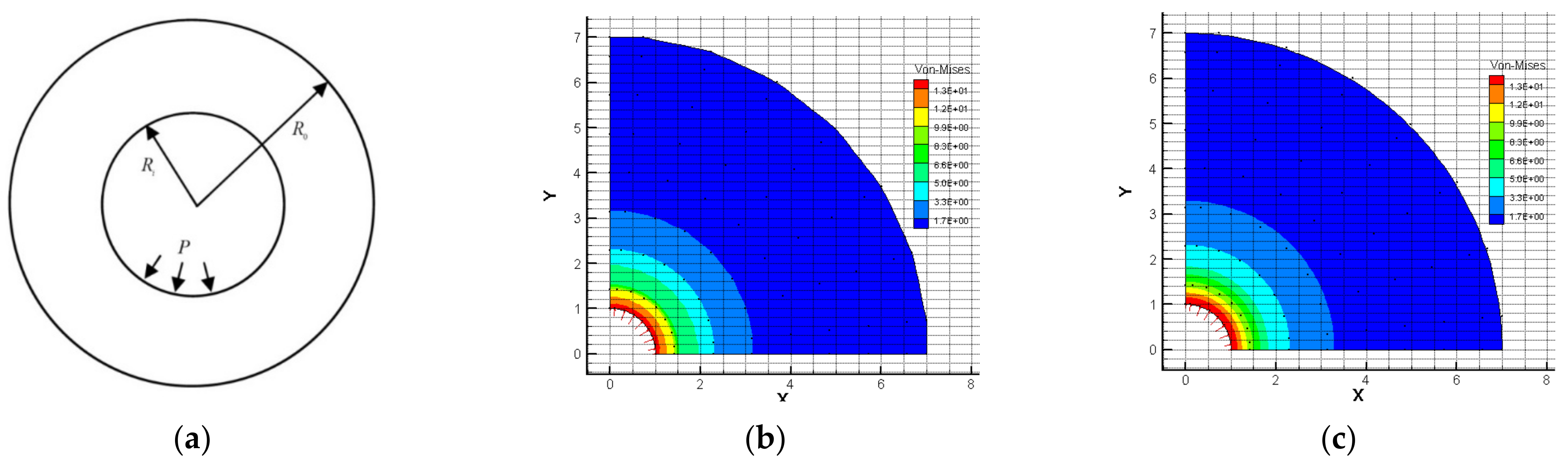
A hollow cylinder subjected to inner pressure is considered in Figure 6a. For the comparison with the exact solution, the linear elastic structure problem is considered. On the inner boundary, pressure which has 10 N/m² is applied. The displacement and traction are free on the outer boundary. The Young’s modulus and Poisson’s ratio are$1.0\times {10}^5$(MPa) and $0.3$, respectively. Inner and outer radii are set as 1 and 7 m. Results of the quarter model for both FEM and IGA are shown in Figure 6b,c using 81 elements.

The analytic (exact) solutions to this problem are as follows:

$$u_r\left(r\right)=\frac{1}{E}\frac{P{R}_i^2}{R_0^2-R_i^2}\left(\left(1-\nu \right)r+\frac{R_0^2\left(1+\nu \right)}{r}\right)$$

(42)

The error norm between the numerical results (FEM and IGA) and the analytic solution is considered to assess the convergence characteristics. The $L_2$ error norm is defined on the internal domain:

$$e=\sqrt{{\displaystyle {\int }_{\mathsf{\Gamma }}^{}{\left|u_{Numerical}-u_{Analytic}\right|}^{2}d\mathsf{\Gamma }}}$$

(43)

Figure 7 compares the error norm of FEM and IGA with the number of elements. Because of the exact geometry and higher continuity between elements in IGA, the convergence of the isogeometric method is faster than that of FEM.

Next, to investigate the convergence of the isogeometric shape design sensitivity, the previous example is considered again. The inner radius is chosen as a design variable, and the analytic exact design sensitivity is derived as follows:

$$\frac{D{u}_r\left(r\right)}{D{R}_i}=\frac{1}{E}\frac{2P{R}_i{R}_0^2}{{\left(R_0^2-R_i^2\right)}^2}\left(\left(1-\nu \right)r+\frac{R_0^2\left(1+\nu \right)}{r}\right)\hspace{0.33em}+\frac{1}{E}\frac{P{R}_i^2}{R_0^2-R_i^2}\left(\left(1-\nu \right)-\frac{R_0^2\left(1+\nu \right)}{r^2}\right)$$

(44)

The convergence of the two methods is shown in Figure 8, and the isogeometric approach converges faster than FEM. Such results can be attributed the higher-order geometric term (normal vector), which can be obtained in the isogeometric method even with using fewer DOFs.

3.3. Shape Design Optimization of Structures Subject to Pressure Load

Utilizing accurate and efficient design sensitivity, shape optimization is performed for the various problems. Under the constraint, the objective function such as compliance is minimized using the MMFD algorithm. For the comparison, FEM, IGA, and linear elasticity-based optimization results are presented. The material properties of the steel were the same used in the previous problem.

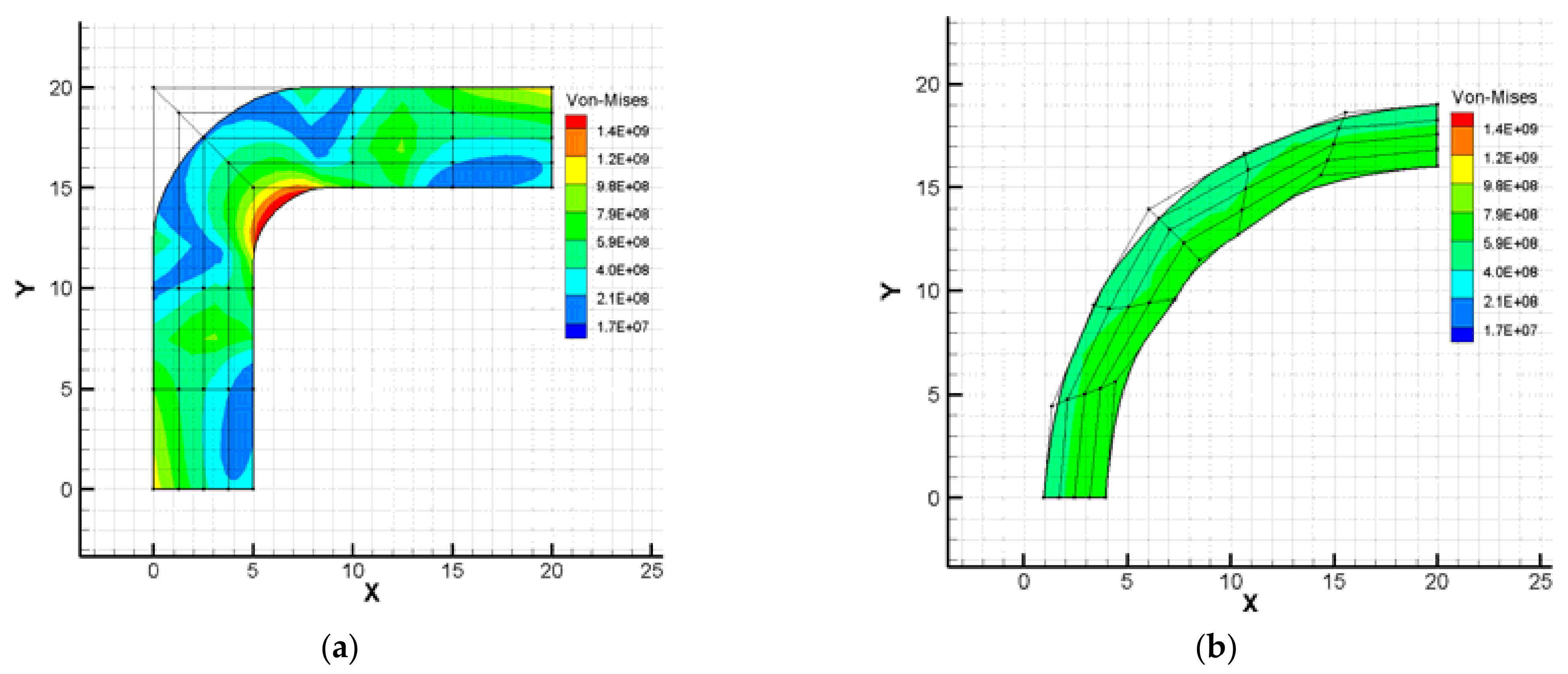
3.3.1. L-Shape Structure

The shape design optimization to minimize compliance at the (n+1) configuration is stated as follows:

$$\mathrm{Minimize} C={\displaystyle {\int }_{\mathsf{\Omega }}^{}p{}^{n+1}u{}_i{}^{n+1}n{}_{i}d\mathsf{\Gamma }}$$

(45)

$$\mathrm{Subject} \mathrm{to} V={\displaystyle {\int }_{\mathsf{\Omega }}d\mathsf{\Omega }\le 0.5\times V_{initial}}$$

(46)

$$d_i^{lower}\le d_i\le d_i^{upper}$$

(47)

where $d_i$ is a shape design variable, i.e., control points along the design boundary. The L-shaped structure with a height of 20 m and thickness of 5 m was selected for the numerical example as shown in Figure 9a. Pressure is applied on the outer boundary, and the symmetry condition is imposed, which is represented by the circular shape ‘o’ in Figure 9a. Design variables are on the inner and outer boundary as blue-colored control points in Figure 9b. The material used is steel, which is defined in Section 3.1. The shape sensitivity of Equations (45) and (46) can be derived using ${}^{n+1}\dot{u}$ from Equation (38) as follows:

$$C^{\prime }={\displaystyle {\int }_{\mathsf{\Omega }}^{}\left(p{}^{n+1}{\dot{u}}_i{n}_i+p{}^{n+1}\dot{u}{}_{i,i}{V}_j{n}_j\right)d\mathsf{\Omega }},$$

(48)

$${\left(Vol\right)}^{\prime }={\displaystyle {\int }_{\mathsf{\Omega }}{V}_{j,j}d\mathsf{\Omega }},$$

(49)

where $V_i$ is a shape design velocity.

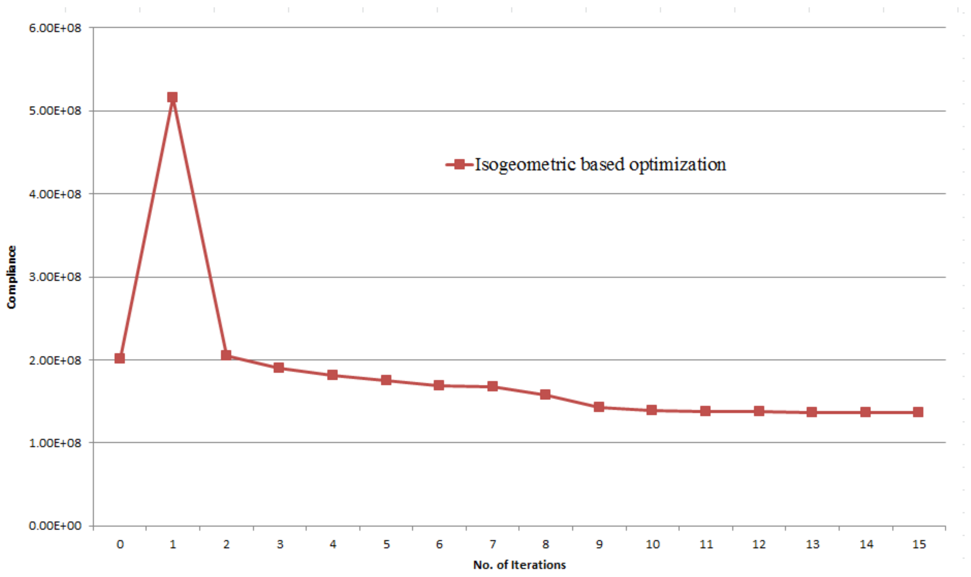
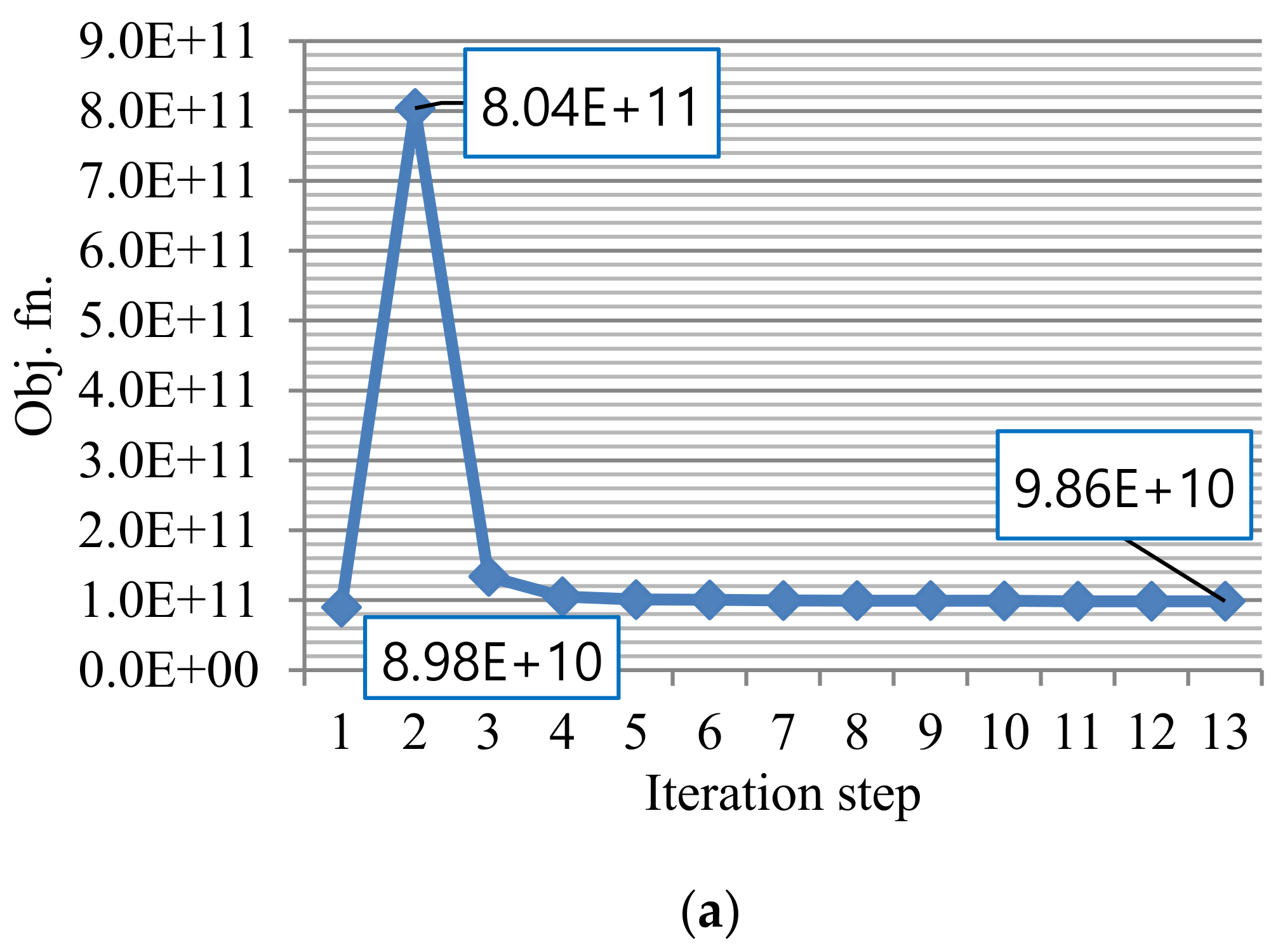
Figure 10 shows the stress distribution of the initial and optimized model. In the initial model, stress concentration occurs at the inner corner. On the contrary, the optimal shape has a round one, and therefore uniform stress distribution is observed. The optimization history of compliance is shown in Figure 11. The compliance is decreased by about 32% from the initial compliance of $2.011\times {10}^8$ to $1.368\times {10}^8$ after 15 design iterations.

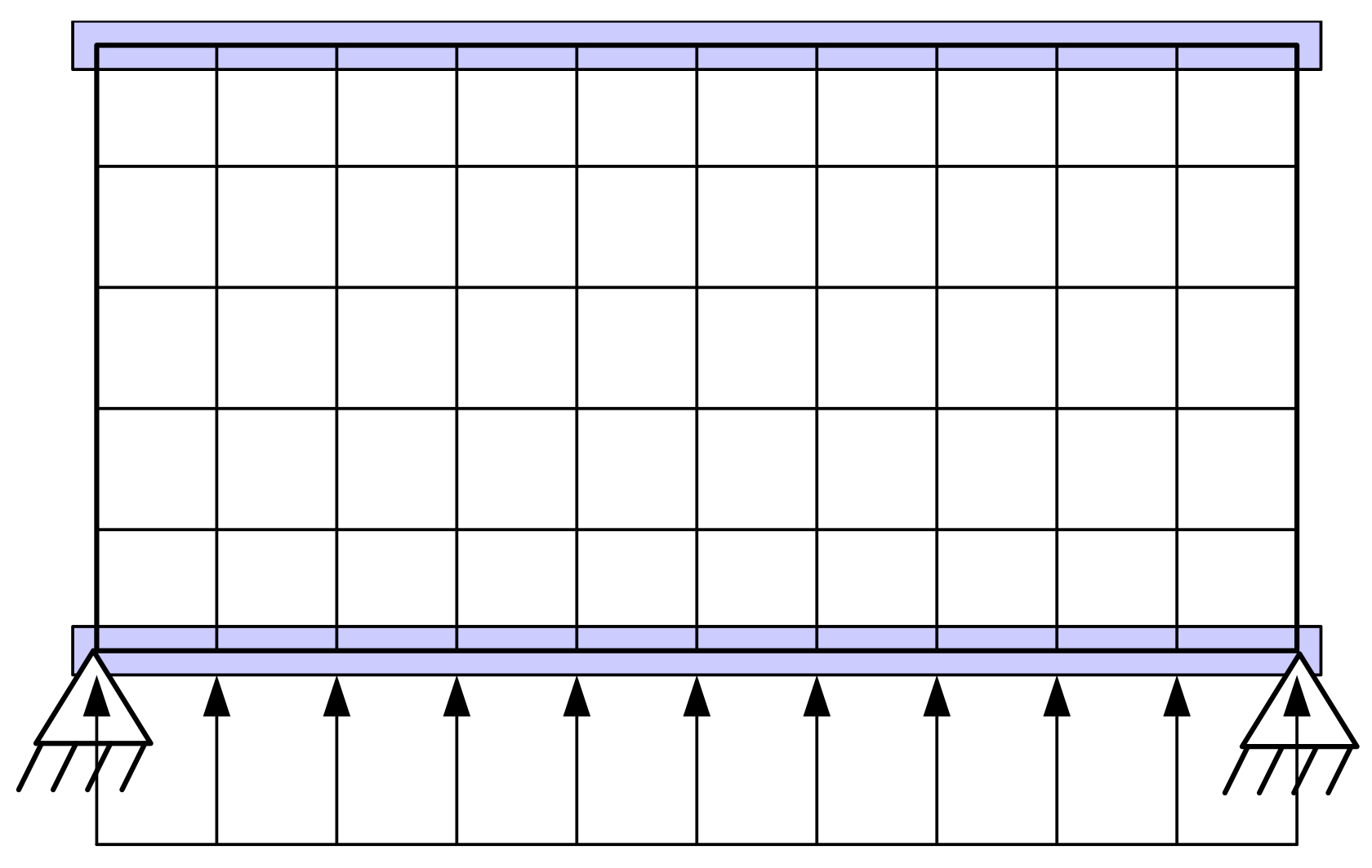
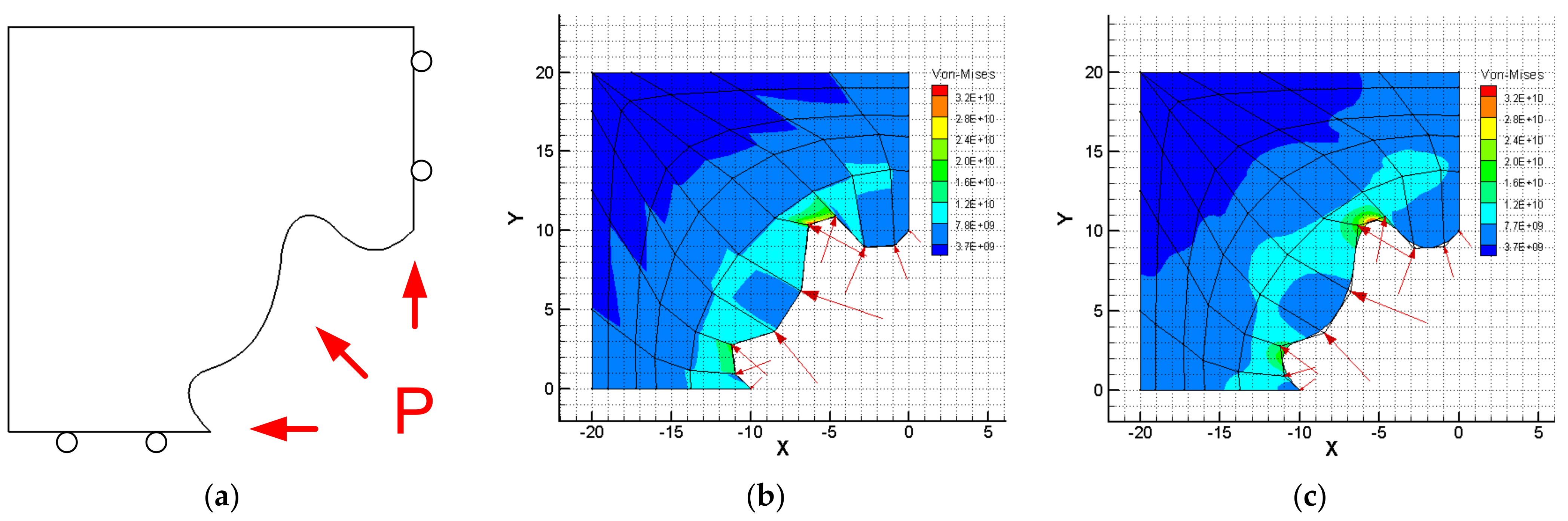
3.3.2. Rectangular Plate

In this example, the shape design optimization of a rectangular structure with a width of 20 m and a height of 10 m considering linear and nonlinear elasticity is performed. The numerical model and design boundary are described in Figure 12. The pressure loading is applied on the lower boundary, and both ends are simply supported, which is represented by the triangle in Figure 12. The material used is steel, which is defined in Section 3.1. The objective function is compliance, and the allowable volume is 60% of the initial one.

Figure 13 shows the optimal shapes for both problems, which have a round shape to resist pressure loads. The optimized shape in Figure 13a has a wiggly lower boundary, which is obtained with consideration of a design-dependent load based on a linear elastic formulation [12,13]. However, the optimized shape considering the design- and deformation-dependent load in the geometrically nonlinear formulation shows a smoother lower boundary where the pressure loading is applied. 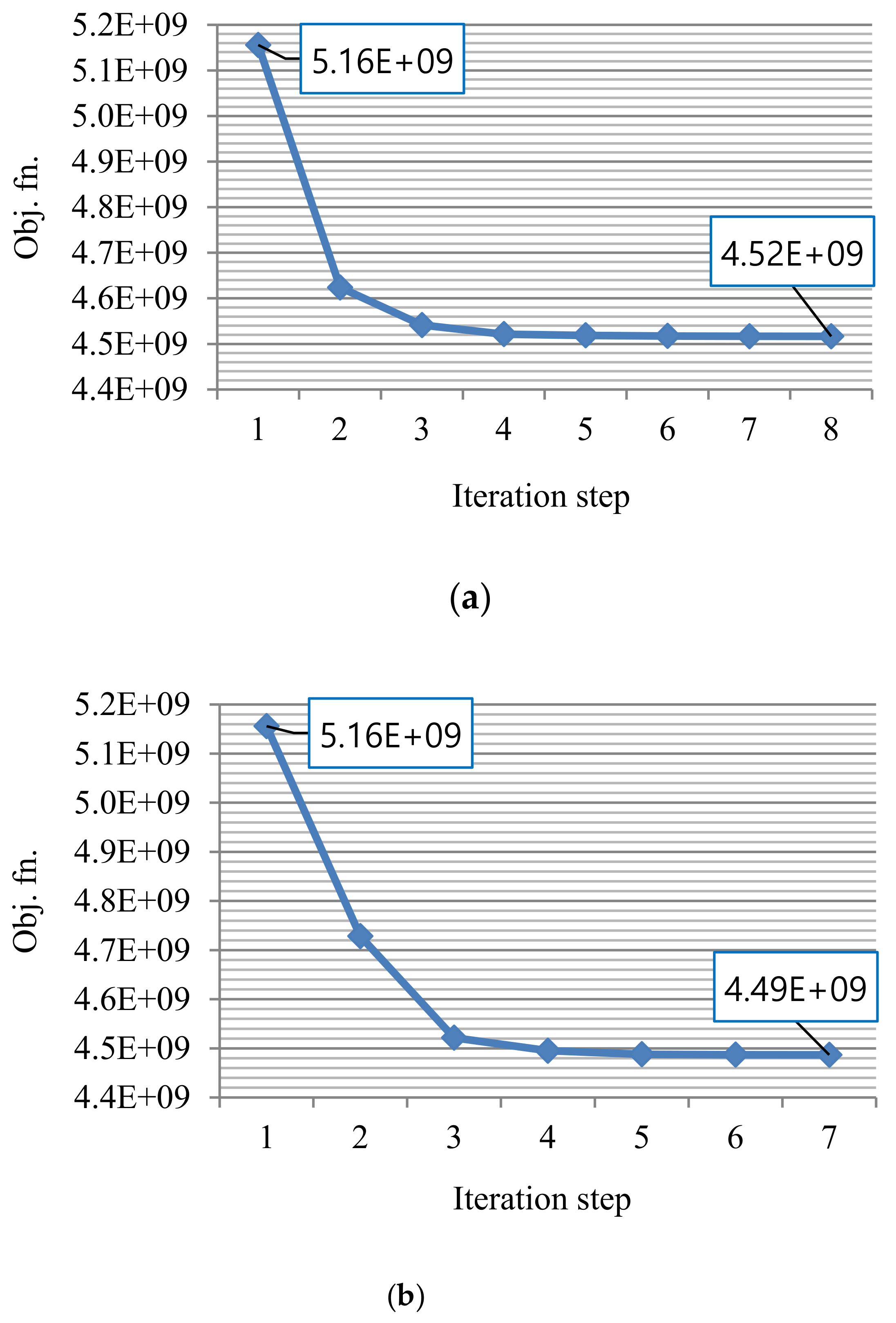Optimization histories for both problems are presented in Figure 14. Since the MMFD algorithm meets the constraint first, it is observed that the objective function goes up first in the second step. From the next step, 60% volume is maintained, satisfying the constraint. Although only 60% of the initial mass can be used, it can be seen that it has similar compliance compared to the initial one.

3.3.3. Irregular Shape Plate

In this example, FEM- and IGA-based shape design optimization is performed. A quarter model of a 5 m × 5 m plate with an irregular inner hole and design boundary is described in Figure 15. The pressure loading is applied on the irregular boundary, which is the design boundary, and the roller boundary condition is imposed on the lower and right sides. The material used is steel, which is defined in Section 3.1. The objective function is compliance, and the allowable volume is the initial one.

As expected, the optimal boundary shape subjected to pressure loading is round, and Figure 16 shows a round optimal shape in both methods. However, the IGA-based optimal shape shows a smoother boundary represented by NURBS.

Optimization histories for both problems are shown in Figure 17. Compliance of the IGA-based optimal shape is slightly lower compared to that of FEM.

4. Conclusions

In the present study, design sensitivity analysis and shape optimization were performed on nonlinear structures subjected to loads that depend on design change and structural deformation. General non-conservative loads have path-dependent properties, and in this paper, the pressure loads are expressed in a total Lagrangian formulation. The resultant load stiffness matrix is derived by linearization, and a tangential stiffness matrix with an asymmetric structure is also derived in the present study. The asymmetric load stiffness term is identified in the continuum-based shape sensitivity formulation to the problems subject to deformation-dependent loads. In addition, since the total Lagrangian formulation was used, no additional iterations are required in the design sensitivity analysis using the final tangential stiffness matrix converged in the nonlinear analysis. In terms of optimization, since normal vectors, which are high-order geometrical terms, can be accurately obtained based on geometrical geometry, it shows an excellent convergence rate even for the problem of a structure under pressure loading, which is expressed with normal vectors of boundaries. Finally, there was no need for design parameterization and smooth design changes by the design variables, as the NURBS basis function was used in optimizing geometry. Analyses in the present study suggest the superiority of the isogeometric optimization technique, which demonstrates the fast convergence with more accurate calculations of the load stiffness terms as well as the normal vector of the pressure load.

References

1. Hibbit, H. Some follower forces and load stiffness. Int. J. Numer. Methods Eng. 1979, 14, 937–941. [Google Scholar] [CrossRef]
2. Mok, D.; Wall, W.; Bischoff, M.; Ramm, E. Algorithmic aspects of deformation dependent loads in non-linear static finite element analysis. Eng. Comput. 1999, 16, 601–618. [Google Scholar] [CrossRef]
3. Simo, J.; Taylor, R.; Wriggers, P. A note on finite-element implementation of pressure boundary loading. Commun. Appl. Numer. Methods 1991, 7, 513–525. [Google Scholar] [CrossRef]
4. Kim, N.H.; Choi, K.K.; Chen, J.S. Die shape design optimization of sheet metal stamping process using meshfree method. Int. J. Numer. Methods Eng. 2001, 51, 1385–1405. [Google Scholar] [CrossRef]
5. Akbari, J.; Kim, N.H.; Ahmadi, M. Shape sensitivity analysis with design-dependent loadings—equivalence between continuum and discrete derivatives. Struct. Multidiscip. Optim. 2010, 40, 353–364. [Google Scholar] [CrossRef]
6. Hammer, V.B.; Olhoff, N. Topology optimization of continuum structures subjected to pressure loading. Struct. Multidiscip. Optim. 2000, 19, 85–92. [Google Scholar] [CrossRef]
7. Kiendl, J.; Schmidt, R.; Wüchner, R.; Bletzinger, K.-U. Isogeometric shape optimization of shells using semi-analytical sensitivity analysis and sensitivity weighting. Comput. Methods Appl. Mech. Eng. 2014, 274, 148–167. [Google Scholar] [CrossRef]
8. Picelli, R.; Neofytou, A.; Kim, H.A. Topology optimization for design-dependent hydrostatic pressure loading via the level-set method. Struct. Multidiscip. Optim. 2019, 60, 1313–1326. [Google Scholar] [CrossRef] [Green Version]
9. Hughes, T.; Cottrell, J.; Bazilevs, Y. Isogeometric analysis: CAD, finite elements. NURBS Exact Geom. Mesh Refinement Comput. Methods Appl. Mech. Eng. 2004, 880, 4135–4195. [Google Scholar]
10. Wall, W.A.; Frenzel, M.A.; Cyron, C. Isogeometric structural shape optimization. Comput. Methods Appl. Mech. Eng. 2008, 197, 2976–2988. [Google Scholar] [CrossRef]
11. Qian, X. Full analytical sensitivities in NURBS based isogeometric shape optimization. Comput. Methods Appl. Mech. Eng. 2010, 199, 2059–2071. [Google Scholar] [CrossRef]
12. Yoon, M.-H.; Koo, B.-Y.; Ha, S.-H.; Cho, S.-H. Isogeometric Shape Design Optimization of Structures Subjected to Design-dependent Loads. J. Comput. Struct. Eng. Inst. Korea 2011, 24, 1–7. [Google Scholar]
13. Pal, A.; Rakshit, S. Isogeometric shape optimization for design dependent loads. J. Comput. Inf. Sci. Eng. 2021, 85376, 1–13. [Google Scholar] [CrossRef]
14. Cho, S.; Ha, S.-H. Isogeometric shape design optimization: Exact geometry and enhanced sensitivity. Struct. Multidiscip. Optim. 2008, 38, 53. [Google Scholar] [CrossRef]
15. Komkov, V.; Choi, K.K.; Haug, E.J. Design Sensitivity Analysis of Structural Systems; Academic Press: Salt Lake City, UT, USA, 1986; Volume 177. [Google Scholar]
16. Choi, K.K.; Kim, N.-H. Structural Sensitivity Analysis and Optimization 1: Linear Systems; Springer Science & Business Media: London, UK, 2004. [Google Scholar]
17. Braibant, V.; Fleury, C. Shape optimal design using B-splines. Comput. Methods Appl. Mech. Eng. 1984, 44, 247–267. [Google Scholar] [CrossRef]
18. Azegami, H.; Shimoda, M.K.S. Katamine E Irregularity of shape design optimization problems and an improvement technique. In Proceedings of the international conference on computer aided optimum design of structures, OPTI, Orlando, FL, USA, 16–18 March 1977; pp. 309–326. [Google Scholar]
19. Vanderplaats, G.N. An efficient feasible directions algorithm for design synthesis. AIAA J. 1984, 22, 1633–1640. [Google Scholar] [CrossRef]
Figure 1. Pressure load: (a) fixed, (b) design-dependent, (c) design- and deformation-dependent.
Symmetry 13 02373 g001
Figure 2. Pressure boundary and differential area element.
Symmetry 13 02373 g002
Figure 3. (a) Isogeometric model description; (b) perturbed red-colored shape (scaled by 100).
Symmetry 13 02373 g003
Figure 4. Dam model: (a) problem description, (b) analysis result, (c) design velocity field.
Symmetry 13 02373 g004
Figure 5. Agreement of FDM and DDM (%) according to various pressure intensity and perturbation amount.
Symmetry 13 02373 g005
Figure 6. (a) Circular cylinder with internal pressure, (b) FEM result, (c) isogeometric result.
Symmetry 13 02373 g006
Figure 7. Comparison of error displacement according to the number of elements used.
Symmetry 13 02373 g007
Figure 8. Comparison of error sensitivity according to the number of elements used.
Symmetry 13 02373 g008
Figure 9. (a) Model description, (b) isogeometric model and blue colored control points as shape design variables.
Symmetry 13 02373 g009
Figure 10. Von mises stress: (a) initial model, (b) optimized model.
Symmetry 13 02373 g010
Figure 11. Optimization history of L-shaped structure.
Symmetry 13 02373 g011
Figure 12. Simply supported rectangular plate and its blue-colored design boundary.
Symmetry 13 02373 g012
Figure 13. Optimal shape: (a) linear elastic problem, (b) geometrically nonlinear elasticity.
Symmetry 13 02373 g013
Figure 14. Optimization history: (a) linear elastic problem, (b) geometrically nonlinear elasticity.
Symmetry 13 02373 g014aSymmetry 13 02373 g014b
Figure 15. (a) Irregular shaped boundary, (b) FEM results, (c) IGA results.
Symmetry 13 02373 g015
Figure 16. Optimal shape: (a) FEM, (b) IGA.
Symmetry 13 02373 g016
Figure 17. Optimization history: (a) FEM, (b) IGA.
Symmetry 13 02373 g017